Accurate, efficient and simple forces with Quantum Monte Carlo methods

Abstract

Computation of ionic forces using quantum Monte Carlo methods has long been a challenge. We introduce a simple procedure, based on known properties of physical electronic densities, to make the variance of the Hellmann-Feynman estimator finite. We obtain very accurate geometries for the molecules H₂, LiH, CH₄, NH₃, H₂O and HF, with a Slater-Jastrow trial wave function. Harmonic frequencies for diatomics are also in good agreement with experiment. An antithetical sampling method is also discussed for additional reduction of the variance.

The optimization of molecular geometries and crystal structures and ab initio molecular dynamics simulations are among the most significant achievements of single particle theories. These accomplishments were both possible thanks to the possibility of readily computing forces on the ions within the framework of the Born-Oppenheimer approximation. The approximate treatment of electron interactions typical of these approaches can, however, lead to quantitatively, and sometimes qualitatively, wrong results. This fact, together with a favorable scaling of the computational cost with respect to the number of particles, has spurred the development of stochastic techniques, i.e. quantum Monte Carlo (QMC) methods. Despite the higher accuracy achievable for many physical properties, the lack of an efficient estimator for forces has prevented, until recentlyFilippi and Umrigar (2000); Casalegno et al. (2003); Assaraf and Caffarel (2000), the use of QMC methods to predict even the simplest molecular geometry. The chief problem is to have a Monte Carlo (MC) estimator for the force with sufficiently small variance. For example, in all-electron calculations, a straightforward application of MC sampling of the Hellmann-Feynman estimator has infinite variance. This can be easily seen from the definition of the force. For a nucleus of charge $Z$ at the origin, the force can be written, together with its variance, as a function of the charge density $\rho(\mathbf{r})$ as

$$\mathbf{F}=Z\int d\mathbf{r}\rho(\mathbf{r})\frac{\mathbf{r}}{r^{3}}\>;\qquad\sigma^{2}=Z^{2}\int d\mathbf{r}\rho(\mathbf{r})\frac{1}{r^{4}}-F^{2}.$$ (1)

Since the electronic density is finite at the origin, the variance integral diverges.

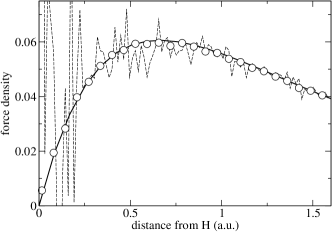
Figure 1: Force density along the z-direction for the H atom in LiH. The bond is along the z-axis, with a length of 3.316 Bohr. The continuous black curve is calculated from the Hartree-Fock orbitals. The dashed line is the estimate of $f_{z}$ using the bare estimator. Circles are obtained in an identical QMC simulation using the antithetic sampling technique outlined in the text.

In this paper, we propose a modified form for the force estimator which has finite variance. This estimator is then used to calculate forces and predict equilibrium geometry and vibrational frequencies for a set of small molecules. Without loss of generality we will consider only the $z$-component of the force on an atom at the origin. In a QMC calculation based in configuration space, the charge density is a sum of delta functions: $\rho(\mathbf{r})\propto\sum_{\mathbf{r}^{\prime}}\delta(\mathbf{r}-\mathbf{r}^{\prime})$, where the sum is over all $N_{e}$ electron positions and all MC samples. We consider separately the electrons within a distance $\mathcal{R}$ of the atom and those outside. The contribution to the force from charges outside, $F_{z}^{O}$, can be calculated directly with the Hellmann-Feynman estimator in Eq. (1). The contribution from inside the sphere is responsible for the large variances in the direct estimator. It is convenient to introduce a “force density” defined as the force arising from electron charges at a distance $r$ from the origin:

$$f_{z}(r)=Z\int d\Omega\;\rho(r,\theta,\phi)\cos\theta$$ (2)

Then the force is given as:

$$F_{z}=F_{z}^{O}+\int_{0}^{\mathcal{R}}f_{z}(r)dr.$$ (3)

The force density is a smooth function of $r$ that tends to $0$ linearly as $r$ approaches the origin. The force density for H in a LiH molecule computed with Hartree-Fock and two different QMC estimators is shown in Fig.1. As expected the bare force estimator fluctuates wildly at small $r$.

Because the force density is a smooth function, we can represent it in the interval $(0,\mathcal{R})$ with a polynomial

$$\widetilde{f_{z}}(r)=\sum_{k=1}^{M}a_{k}r^{k}$$ (4)

and determine the coefficients, $a_{k}$, by minimizing

$$\chi^{2}=\int_{0}^{\mathcal{R}}dr\,r^{m}\left[f_{z}(r)-\widetilde{f_{z}}(r)\right]^{2}$$ (5)

where $r^{m}$ is a weight factor used to balance contributions from different values of $r$.

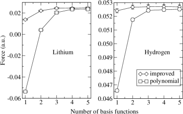
Figure 2: Dependence of the VMC force on the expansion basis, for LiH with a bond length of 3.316 Bohr. The fitting radius $\mathcal{R}=$0.6 Bohr. The definitions of the basis functions are in Eq.’s (4) and (9). The forces on H and Li are different because of the lack of full optimization of the VMC wave function (see text).

Since the relation between the force and the force density is linear, and the relation between the fitting coefficients and the electronic density is linear, we can directly write the force as averages over moments of the force density. After some manipulations we arrive at:

$$F_{z}=F_{z}^{O}+Z\left\langle\sum_{i=1}^{N_{e}}g(r_{i})\frac{z_{i}}{r_{i}^{3}}\right\rangle_{\rm MC},$$ (6)

where the new estimator function is:

$$g(r)=\theta(\mathcal{R}-r)\sum_{k=1}^{M}c_{k}r^{k+m}.$$ (7)

The coefficients $c_{k}$’s are determined by $\mathbf{c}=\mathbf{S^{-1}h}$ where the Hilbert matrix $\mathbf{S}$ and the residual vector $\mathbf{h}$ are

$$S_{kj}=\frac{\mathcal{R}^{m+k+j+1}}{m+k+j+1},\qquad h_{j}=\frac{\mathcal{R}^{j+1}}{j+1}.$$ (8)

Note that for the bare estimator $g(r)=\theta(\mathcal{R}-r)$. Because of the restriction on the basis, the variance of the new estimator is finite as long as $m>-1/2$. We have numerically found that the weighting factor $m=2$, where each volume element is weighted equally, gives the lowest variance estimate of the force.

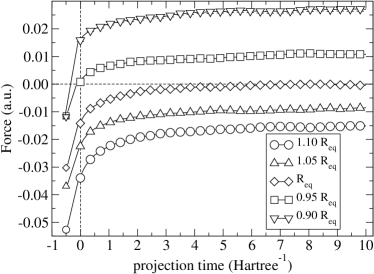
Figure 3: Projection of the force in LiH using forward walking. The points at negative imaginary time give the VMC values. Values at $0$ are the mixed estimates of the DMC simulation.

To derive the estimator we have used the fact that $f_{z}(r)$ goes linearly at small $r$. This is the crucial property that allows to filter out the $s$-wave component of the density responsible for the variance divergence. The original estimator is correct for any arbitrary charge density while the new filtered one uses physical properties of the charge density to reduce the variance. The variance depends on the fitting radius $\mathcal{R}$ and on the basis set size $M$. As $\mathcal{R}$ increases, the size of the basis must increase, which increases the variance. Charge densities corresponding to low energy states must be smooth and we typically find that only 2 or 3 basis functions are needed. The size of the basis can be reduced by using more appropriate basis sets. For example, in all calculations reported below we used the expansion

$$\widetilde{f}_{z}(r)=f^{\text{SD}}_{z}(r)\sum_{k=0}^{M}a_{k}r^{k},$$ (9)

where $f^{\text{SD}}_{z}$ is the force density of a single determinant wave function, which can be readily computed from the orbitals. The improved basis allows a smaller polynomial set and a reduction of the variance. In Fig. 2 the dependence of the bias on the basis set type and size is shown for the case of a variational Monte Carlo (VMC) simulation on LiH at a bond length of $3.316$ Bohr.

The trial wave functions $\Psi_{T}$ used in all cases were of the Slater-Jastrow form. The orbitals were obtained from a Hartree-Fock calculation using CRYSTAL98 Saunders et al. (1998). The electron-electron and electron-proton Jastrow factors had the form of $\exp(ar/(1+br))$, with $a$ and $b$ optimized by minimizing $|E_{loc}-\langle E\rangle|$ Bressanini et al. (2002) over points sampled from $|\Psi_{T}|^{2}$. The time step in the diffusion Monte Carlo (DMC) simulations was chosen to give an acceptance ratio of $98$%, a value for which the time step bias on forces was within the statistical error bars.

Table 1: Equilibrium distances in Å. Experimental, CCSD(T) and B3LYP values were taken from RefCCC (2004). The CCSD(T) and the B3LYP results were obtained using the cc-pVTZ basis set with the exception of LiH where the 6-311G* set was used. PBE results Xu and Goddard (2004) were all obtained using the aug-cc-pVTZ basis set.

	QMC	Exp.	CCSD(T)	B3LYP	PBE
H2	0.7419(4)	0.741	0.743	0.743	0.751
LiH	1.592(4)	1.596	1.618	1.595	1.606
CH4	1.091(1)	1.094	1.089	1.088	1.096
NH3 (N-H)	1.009(2)	1.012	1.014	1.014	1.023
NH3 (H-H)	1.624(2)	1.624	1.616	1.624	1.634
H2O (O-H)	0.959(2)	0.956	0.959	0.961	0.971
H2O (H-H)	1.519(3)	1.517	1.508	1.520	1.531
HF	0.919(1)	0.918	0.917	0.923	0.932

Since the exact density is needed for the Hellmann-Feynman theorem, forward walkingHammond et al. (1994) or one of the variational path integral algorithmsCeperley (1995); Baroni and Moroni (1999) is needed in order to evaluate the force estimator. An example of the convergence of forward walking is shown in Fig. 3. The force as a function of the forward-walking projection time quickly reaches a plateau corresponding to the exact value. In this example, the variational forces are far from correct. This discrepancy results from the lack of full optimization of the trial wave function made of localized basis orbitals and atom centered Jastrow factors, and can be reduced somewhat by including Pulay terms Casalegno et al. (2003). In DMC, forward walking eliminates the need for the Pulay corrections.

The equilibrium geometries were computed by fitting the QMC forces in the proximity of the equilibrium geometry to a polynomial with the appropriate symmetry. Fig. 4 shows the force in hydrogen fluoride in a 2% interval around the equilibrium geometry. The equilibrium geometries are reported in Table 1 together with those given by CCSD(T), DFT using the B3LYP and the PBE functional, and experiments. The differences between QMC and experimental values are in all cases less than $0.4\%$ and closer to the experiment than the other techniques. For diatomics it is easy to provide an estimate of the harmonic vibrational frequencies starting from the derivative of the force curve at equilibrium geometry. The QMC frequencies, reported in Table 2, are in good agreement with the experiment, with errors comparable to that from CCSD(T) and DFT PBE or B3LYP. This suggests that forces computed within our approach are accurate also away from the equilibrium and could be used in molecular dynamics calculations or to optimize molecular geometries.

The only source of systematic error in our calculations that cannot be simply addressed is the fixed-node error. In fixed-node DMC, the random walk is forbidden to cross the nodes of the trial wavefunction in order to prevent the loss of efficiency due to the fermion antisymmetry. If the nodes are accurate, so is the QMC energy and electronic density; hence the force. For incorrect nodes, the energy is an upper bound to the true energy, but such can not be said for the force. It is also not necessarily the case that the forces obtained from Eq. (1) are equal to the gradient of the fixed-node energySchautz and Flad (1999, 2000); Huang et al. (2000): this is only guaranteed in the limit of exact nodal surfaces. The high quality of the geometries and vibrational frequencies suggests that these errors, at least for the cases treated in this paper, are negligible. This is perhaps not surprising, since the electronic density is a 1-electron property, while the nodal error is a many-body effect.

Table 2: Harmonic frequencies in cm^-1. Experimental, CCSD(T) and B3LYP values were taken from RefCCC (2004). The CCSD(T) and the B3LYP results were obtained using the cc-pVTZ basis set with the exception of LiH where the 6-311G* set was used. PBE results Patton et al. (1997) were obtained using ad hoc gaussian basis sets.

	QMC	Exp.	CCSD(T)	B3LYP	PBE
H2	4464(18)	4410	4420	4401	4323
LiH	1445(20)	1369	1414	1405	1380
HF	4032(266)	4181	4085	4138	4001

We have also tested another method to further reduce the variance of the Hellmann-Feynman estimator. The filtered estimator performs well on the hydrogen atom but for heavier nuclei the error bar grows and seems to scale as $Z^{3}$. In those cases the new method can potentially be very useful, with error bars scaling between $Z$ and $Z^{2}$. The method is based on the observation that, while electrons in the core cause large fluctuations in the force density, they contribute very little to it. A standard approach to reduce the variance of a Monte Carlo estimate is the use of antithetic variatesKalos and Whitlock (1986): a positive fluctuation is paired with a negative fluctuation. Suppose the random walk arrives at a multidimensional electronic configuration $R$, with $p$ ($\geq 1$) electrons inside a radius $\mathcal{R}_{av}\leq\mathcal{R}$ of an atom located at the origin. We obtain an antithetic configuration $R^{\prime}$ by reflecting all $p$ core electrons about the origin. We then estimate the force contribution due to the $p$ electrons using both $R$ and $R^{\prime}$, assigning a weight factor of $w(R^{\prime})=|\psi(R^{\prime})/\psi(R)|^{2}$ to $R^{\prime}$. Their joint contribution to the estimator in Eq. (6) is $Z\frac{1-w(R^{\prime})}{2}\sum_{i}g(r_{i})z_{i}r^{-3}$ where the sum runs over the $p$ core electrons. Since $w\rightarrow 1$ as $\mathcal{R}_{av}\rightarrow 0$, fluctuations in the core are much reduced.

Within VMC this scheme can be implemented exactly, leading to a dramatic reduction of the variance as can be noticed from Fig. 1. However this estimator is non-local and, in DMC, suffers from the same problems as non-local pseudopotentials, making an unbiased implementation not straightforward. We postpone further discussion of the antithetic method to a future article.

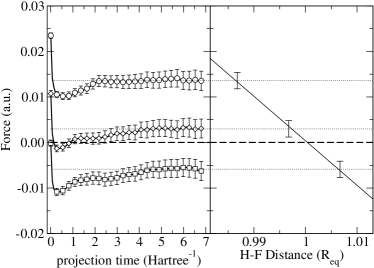
Figure 4: DMC force in hydrogen fluoride. Left panel: evolution of the force over forward-walking time. Right panel: fully projected forces as a function of nuclear distance. R${}_{\text{eq}}$ is the experimental equilibrium distance.

Two other approaches have been introduced recently for the computation of forces in QMC. Filippi and Umrigar have computed forces for diatomics by correlating random walks for interatomic separations $a$ and $a^{\prime}$. In DMC the difficulty associated with the nodal error and the branching factor was overcome by neglecting some types of correlation. The main drawback of a finite difference method is the difficulty of calculating all the components of the force simultaneously; for a system of $N$ atoms this method would require $3N$ separate force calculations.

The other approach, introduced in Ref. Assaraf and Caffarel (2000), is closer to our method. It is based on a “zero-variance” version of the Hellmann-Feynman estimator and can be understood in the framework of this paper: one can prove that it corresponds to filtering out the $s$-wave component of the density leaving the force density unchanged. The semi-local character of the “zero-variance” estimator makes its DMC implementation trickier. To overcome this problem there have been attemptsCasalegno et al. (2003); Assaraf and Caffarel (2003) to use correction terms similar in nature to the Pulay terms in single-particle approaches. In practice, this scheme requires extensive optimization and, although promising, it is unclear if it will be viable for more complicated cases. In addition, the value of the force is very sensitive to small errorsAssaraf and Caffarel (2003) in the charge density and the optimization within a stochastic technique is probably not sufficiently stable to eliminate these errors.

In conclusion, we have developed a simple method for computing forces within quantum Monte Carlo and used it to find the equilibrium geometries for small polyatomic molecules. This has been the first time that a QMC technique is used to predict geometries of molecules beyond diatomics. The only overhead in the calculation is the necessity of determining unbiased estimators, which requires the use of either forward-walking or reptation MC techniques. The new method leads to very accurate forces despite errors from the fixed-node approximation and from its contribution to the energy derivatives. Extension of the method, including the antithetic estimator technique, to heavier atoms and to atoms with pseudopotentialsis under investigation.

This material is based upon work supported in part by the U.S Army Research Office under DAAD19-02-1-0176. Computational support was provided by the Materials Computational Center and the National Center for Supercomputing Applications at the University of Illinois. S.Z. acknowledges support from NSF.

References

- Filippi and Umrigar (2000) C. Filippi and C. J. Umrigar, Phys. Rev. B 61, R16291 (2000).
- Casalegno et al. (2003) M. Casalegno, M. Mella, and A. M. Rappe, J. Chem. Phys. 118, 7193 (2003).
- Assaraf and Caffarel (2000) R. Assaraf and M. Caffarel, J. Chem. Phys. 113, 4028 (2000).
- Saunders et al. (1998) V. R. Saunders, R. Dovesi, C. Roetti, M. Causa, N. M. Harrison, R. Orlando, and C. M. Zicovich, CRYSTAL98 User’s Manual, University of Torino (1998).
- Bressanini et al. (2002) D. Bressanini, G. Morosi, and M. Mella, J. Chem. Phys. 116, 5345 (2002).
- CCC (2004) Computational chemistry comparison and bechmark database, http://srdata.nist.gov/cccbdb/ NIST Standard Reference Database (2004).
- Xu and Goddard (2004) X. Xu and W. A. Goddard, J. Chem. Phys. 121, 4068 (2004).
- Hammond et al. (1994) B. L. Hammond, W. A. Lester, and P. J. Reynolds, Monte Carlo Methods in Ab Initio Quantum Chemistry (World Scientific, 1994).
- Ceperley (1995) D. Ceperley, Rev. Mod. Phys. 67, 279 (1995).
- Baroni and Moroni (1999) S. Baroni and S. Moroni, Phys. Rev. Lett. 82, 4745 (1999).
- Schautz and Flad (1999) F. Schautz and H. J. Flad, J. Chem. Phys. 110, 11700 (1999).
- Schautz and Flad (2000) F. Schautz and H. J. Flad, J. Chem. Phys. 112, 4421 (2000).
- Huang et al. (2000) K. C. Huang, R. J. Needs, and G. Rajagopal, J. Chem. Phys. 112, 4419 (2000).
- Patton et al. (1997) D. C. Patton, D. V. Porezag, and M. R. Pederson, Phys. Rev. B 55, 7454 (1997).
- Kalos and Whitlock (1986) M. H. Kalos and P. A. Whitlock, Monte Carlo Methods. Volume I: Basics (John Wiley & Sons, 1986).
- Assaraf and Caffarel (2003) R. Assaraf and M. Caffarel, J. Chem. Phys. 119, 10536 (2003).