Counterion density profiles at charged flexible membranes

Abstract

Counterion distributions at charged soft membranes are studied using perturbative analytical and simulation methods in both weak coupling (mean-field or Poisson-Boltzmann) and strong coupling limits. The softer the membrane, the more smeared out the counterion density profile becomes and counterions pentrate through the mean-membrane surface location, in agreement with anomalous scattering results. Membrane-charge repulsion leads to a short-scale roughening of the membrane.

The study of charged colloids and biopolymers faces a fundamental problem: In theoretical investigations, the central object which is primarily computed is the charge density distribution in the electrolyte solution adjacent to the charged body book . Experimentally measurable observables are typically derived from this charge distribution. For example, the force between charged particles follows from the ion density at the particle surfaces via the contact-value theorem. Likewise, the surface tension and surface potential are obtained as weighted integrals over the ion distributions. It has proven difficult to measure the counterion distribution at a charged surface directly because of the small scattering intensity. Notable exceptions are neutron scattering contrast variation with deuterated and protonated organic counterions scatter1 and local fluorescence studies on Zinc-ion distributions using X-ray standing waves scatter2 . Clearly, direct comparison between theoretical and experimental ion distributions (rather than derived quantities) is desirable as it provides important hints how to improve theoretical modeling.

In a landmark paper the problem of low scattering intensity was overcome by anomalous X-Ray scattering on stacks of highly charged bilayer membranes Richardsen et al. (1996). Anomalous scattering techniques allow to sensitively discriminate counterion scattering from the background, and a multilayer consisting of thousands of charged layers gives rise to substantial scattering intensity. Since then, similar techniques have been applied to charged biopolymers Doniach ; Wong and to oriented charged bilayer stacks, where the problem of powder-averaging is avoided Tim .

However, scattering on soft bio-materials brings in a new complication, not considered theoretically so far: soft membranes and biopolymers fluctuate in shape, and thus perturb the counterion density profile. Comparison with standard theories for rigid charged objects of simple geometric shape becomes impossible. Here we fill this gap by considering the counterion-density profile close to a planar charged membrane which exhibits shape fluctuations governed by bending rigidity. As main result, we derive for a relatively stiff membrane closed-form expressions for the counterion density profile in the asymptotic low and high-charge limits which compare favorably with our simulation results. These parametric profiles, which exhibit a crucial dependence on the membrane stiffness, will facilitate the analysis of scattering results since they allow for a data fit with only a very few physical parameters. In previous experiments, a puzzling ion penetration into the lipid region was detected but interpreted as an artifact Richardsen et al. (1996). We show that ion penetration indeed occurs and is due to the correlated ion-membrane spatial fluctuations. The electrostatic coupling between membrane charges and counterions not only modifies the counterion density profile but also renormalizes the membrane roughness: the short-scale bending rigidity is reduced, charged membranes become locally softer.

The Hamiltonian $H=H_{m}+H_{e}$ of the membrane-counterion system consists of the elastic membrane part $H_{m}$ and the electrostatic part $H_{e}$. We discretize the membrane shape on a two-dimensional $N_{L}\times N_{L}$ square lattice with lattice constant $a$ and rescale all lengths by the Gouy-Chapman length $\mu=1/2\pi q\ell_{B}\sigma_{m}$ according to $\mathbf{r}=\mu\tilde{\mathbf{r}}$, where $\sigma_{m}=QM/N_{L}^{2}a^{2}$ is the projected charge density of the membrane and $\ell_{B}=e^{2}/4\pi\varepsilon_{0}\varepsilon k_{B}T$ is the Bjerrum length ($e$ is the elementary charge, $\varepsilon$ the dielectric constant). Parametrizing the membrane shape by the height function $h({\bf x})$, the elastic membrane energy in harmonic approximation reads in units of $k_{B}T$ Lip :

$$H_{m}[\tilde{h}] = \frac{K_{0}}{2}\int d^{2}\tilde{x}\,\left(\Delta\tilde{h}(\tilde{\mathbf{x}})\right)^{2}+\frac{\tilde{g}}{2}\int d^{2}\tilde{x}\,\tilde{h}^{2}(\tilde{\mathbf{x}}),$$ (1)

where $\Delta$ is the Laplace operator, $K_{0}$ is the bare bending rigidity and $\tilde{g}=g\mu^{4}$ is the rescaled strength of the harmonic potential. The electrostatic energy accounts for the interaction of $N$ counter-ions of valence $q$ and $M$ membrane charges of valence $Q$, related by the electroneutrality condition $QM=qN$,

$$H_{e} = \sum_{i=1}^{N-1}\sum_{j=i+1}^{N}\frac{\Xi}{\left|\tilde{\mathbf{r}}_{i}-\tilde{\mathbf{r}}_{j}\right|}-$$ (2)

$$\sum_{i=1}^{N}\sum^{M}_{k=1}\frac{Q/q\Xi}{\left|\tilde{\mathbf{r}}_{i}-\tilde{\mathbf{R}}_{k}\right|}+\sum^{M-1}_{k}\sum^{M}_{l=k+1}\frac{(Q/q)^{2}\Xi}{\left|\tilde{\mathbf{R}}_{k}-\tilde{\mathbf{R}}_{l}\right|}$$

where $\Xi=2\pi q^{3}\ell_{B}^{2}\sigma_{m}$ denotes the coupling parameter moreira02a . The rescaled position of the $i$th counterion is $\tilde{\mathbf{r}}_{i}$ while the $k$-th membrane-ion is located at $\tilde{\mathbf{R}}_{k}=(\tilde{\mathbf{x}}_{k},\tilde{h}(\tilde{\mathbf{x}}_{k})-\tilde{d})$ where the membrane charges are displaced by $\tilde{d}=2\tilde{a}N_{L}M^{-1/2}$ beneath the membrane surface which is impenetrable to the point-like counterions. This way we can largely neglect charge-discreteness effects Moreira and Netz (2002a) and concentrate on shape-fluctuation effects. In most of our simulations the membrane ions are mobile and move freely on the membrane lattice, with a packing fraction $\zeta=M/N^{2}_{L}$. For the long-ranged electrostatic interactions we employ laterally periodic boundary conditions using Lekner-Sperb methods moreira02a . To minimize discretization and finite-size effects, the number of lattice sites $N_{L}$ and the rescaled strength of the harmonic potential $\tilde{g}$ are chosen such that the lateral height-height correlation length of the membrane $\xi^{0}_{\parallel}$ obeys the inequality: $\tilde{a}<\tilde{\xi}^{0}_{\|}=(4K_{0}/\tilde{g})^{1/4}\ll N_{L}\tilde{a}$Lip . Simulations are run for typically $10^{6}$ Monte Carlo steps using 100 counter-ions and 100 membrane ions. In Fig.1 we show two simulation snapshots. The counter-ions form in the weak coupling limit ($\Xi=0.2$, Fig.1.a) a diffuse dense cloud while in the strong coupling limit ($\Xi=1000$, Fig.1.b, note the anisotropic rescaling) the lateral ion-ion distances are large compared to the mean separation from the membrane. Pronounced correlations between membrane shape fluctuations and counterion positions are observed in both snapshots.

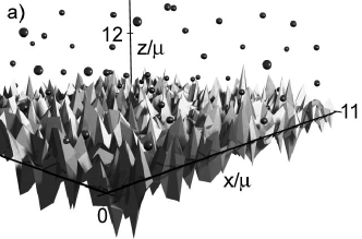
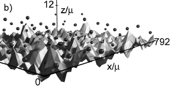
Figure 1: Simulation snapshots for a) $\Xi=0.2$, $\xi^{0}_{\bot}/\mu=0.80$, $K_{0}=0.07$, $\tilde{g}=0.57$, $\tilde{a}=0.18$, $\tilde{d}=2.2$ and b) $\Xi=1000$, $\xi^{0}_{\bot}/\mu=0.38$, $K_{0}=174$, $\tilde{g}=0.006$, $\tilde{a}=13.21$, $\tilde{d}=160$. The simulations are done using $N=100$ counter-ions and $M=100$ membrane-ions on a $N_{L}=60\times 60$ membrane lattice.

The qualitatively different ionic structures at low/high coupling strength are reflected by fundamentally different analytic approaches in these two limits: Starting point is the exact expression for the partition function

$$\mathcal{Z}=\int\mathcal{D}\tilde{h}\frac{1}{N!}\prod_{i=1}^{N}\int{d\tilde{\bf x}_{i}}\int_{\tilde{h}(\tilde{\bf x}_{i})}^{\infty}d\tilde{z}_{i}e^{-H}\,.$$ (3)

By performing a Hubbard-Stratonovich transformation and a transformation to the grand-canonical ensemble, we arrive at the partition function henri1 :

$$\mathcal{Z}\simeq\int\mathcal{D}\tilde{h}\mathcal{D}\phi e^{-H_{m}[\tilde{h}]-H_{\phi}[\tilde{h},\phi,\pi]/\Xi}$$ (4)

The field $i\phi$ is the fluctuating electrostatic potential henri1 . The electrostatic action reads

$$H_{\phi}[\tilde{h},\phi,\pi]\!\! = \!\!\frac{1}{8\pi}\!\int\!d\tilde{\mathbf{r}}\,\left(\nabla\phi(\tilde{\mathbf{r}})\right)^{2}\!-\!\frac{i}{2\pi}\!\int\!d\tilde{\mathbf{r}}\,\delta(\tilde{z}-\tilde{h}(\tilde{\mathbf{x}}))\phi(\tilde{\mathbf{r}})$$ (5)

$$-\frac{\Lambda}{2\pi}\!\int\!d\tilde{\mathbf{r}}\,e^{\pi(\tilde{\mathbf{r}})-i\phi(\tilde{\mathbf{r}})}\theta(\tilde{z}-\tilde{h}(\tilde{\mathbf{x}}))$$

where $\theta(z)=1$ for $z>0$ and zero otherwise. The expectation value of the counter-ion density is calculated by the help of the generating field $\pi(\mathbf{r})$ according to $\langle\bar{\rho}(\tilde{\mathbf{r}})\rangle=2\pi\Xi\delta\ln\mathcal{Z}/\delta\pi(\tilde{\mathbf{r}})\mu^{3}$ and reads

$$\left\langle\bar{\rho}(\tilde{\mathbf{r}})\right\rangle=\frac{\left\langle\rho(\tilde{\mathbf{r}})\right\rangle}{2\pi\ell_{B}\sigma_{m}^{2}}=\Lambda\left\langle\theta(\tilde{z}-\tilde{h}(\tilde{\mathbf{x}}))e^{-i\phi(\tilde{\mathbf{r}})}\right\rangle\,.$$ (6)

The dimensionless fugacity $\Lambda$ is determined by the normalization condition of the counterion distribution $\int d\mathbf{r}\,\left\langle\rho(\mathbf{r})\right\rangle=N$, which is in rescaled units equivalent to $\Lambda\int d\tilde{\mathbf{r}}\,\left\langle\theta(\tilde{z}-\tilde{h}(\tilde{\mathbf{\mathbf{x}}}))e^{-i\phi(\tilde{\mathbf{r}})}\right\rangle=1$. The partition function Eq.(4) is intractable. In the weak coupling limit, $\Xi\to 0$, fluctuations of the field $\phi$ around the saddle point value are small and gaussian variational methods become accurate henri2 . The variational Gibbs free energy reads:

$$F_{v} = F_{0}+\left\langle H_{\phi}[\tilde{h},\phi,\pi]/\Xi+H_{m}[\tilde{h}]-H_{0}[\tilde{h},\phi]\right\rangle_{0}$$ (7)

Here $\langle\cdots\rangle_{0}$ is an average with the variational hamiltonian $H_{0}$ and $F_{0}$ is the corresponding free energy. The most general Gaussian variational hamiltonian $H_{0}$ is

$$H_{0}[\tilde{h},\phi] = \frac{1}{2}\int d\tilde{\mathbf{x}}d\tilde{\mathbf{x}}\prime\,\tilde{h}(\tilde{\mathbf{\mathbf{x}}})K^{-1}(\tilde{\mathbf{x}},\tilde{\mathbf{x}}\prime)\tilde{h}(\tilde{\mathbf{x}}\prime)$$ (8)

$$+\frac{1}{2}\int d\tilde{\mathbf{r}}d\tilde{\mathbf{r}}\prime\,\Omega(\tilde{\mathbf{r}})v^{-1}(\tilde{\mathbf{r}},\tilde{\mathbf{r}}\prime)\Omega(\tilde{\mathbf{r}}\prime)\,,$$

where the field $\Omega$ is defined by $\Omega(\tilde{\mathbf{r}}):=\phi(\tilde{\mathbf{r}})-\phi_{0}(\tilde{\mathbf{r}})+i\int d\tilde{\mathbf{x}}\prime d\tilde{\mathbf{x}}\prime\prime\,P(\tilde{\mathbf{r}};\tilde{\mathbf{x}}\prime)K^{-1}(\tilde{\mathbf{x}}\prime,\tilde{\mathbf{x}}\prime\prime)\tilde{h}(\mathbf{\tilde{\mathbf{x}}}\prime\prime)$ and $P$ is the connected correlation function $P(\tilde{\mathbf{r}};\tilde{\mathbf{x}}\prime)=\langle i\phi(\tilde{\mathbf{r}})\tilde{h}(\tilde{\mathbf{x}}\prime)\rangle_{0}^{c}$. The variational parameters are the mean potential $\phi_{0}$, the coupling operator $P$, the propagator of the electrostatic field $v$ and the membrane propagator $K$. For $K$ we use the bare propagator of the uncharged membrane $K(\tilde{\mathbf{x}},\tilde{\mathbf{x}}\prime)=-4(\tilde{\xi}^{0}_{\bot})^{2}\mbox{kei}(\sqrt{2}|\tilde{\mathbf{x}}-\tilde{\mathbf{x}}\prime|/\tilde{\xi}^{0}_{\|})/\pi$, where the bare membrane roughness $\xi_{\perp}^{0}$ is given by $1/\sqrt{64K_{0}\tilde{g}}=(\tilde{\xi}^{0}_{\bot})^{2}=\langle\tilde{h}^{2}(0)\rangle_{0}$ Lip . Assuming the charge propagator $v$ to be isotropic and translational invariant (which is an approximation) $v$ turns out to be the bare Coulomb propagator, $v({\bf r})=1/r$. The remaining variational equations $\delta F_{v}/\delta P=\delta F_{v}/\delta\phi_{0}=0$ are solved perturbatively in an asymptotic small $\tilde{\xi}^{0}_{\bot}$ expansion, i.e. for a relatively stiff membrane. The solution for $P$ for $\tilde{\mathbf{x}}=\tilde{\mathbf{x}}\prime$ is expressed in terms of the Meijer’s $\mathcal{G}$ function and reads (neglecting terms of $\mathcal{O}((\tilde{\xi}^{0}_{\bot})^{3})$):

$$P_{\!\bot}(\tilde{z})\!\!=\!\!\frac{-(\tilde{\xi}^{0}_{\bot}\!)^{2}}{\sqrt{2}\pi^{\frac{5}{2}}}\mbox{erf}\!\!\left[\!\frac{\tilde{z}}{\sqrt{2(\tilde{\xi}^{0}_{\bot}\!)^{2}}}\!\right]\!\!\mathcal{G}^{5,1}_{1,5}\!\!\left(\!\!\frac{1}{64}\!\!\left(\!\frac{\tilde{z}}{\tilde{\xi}^{0}_{\|}}\!\right)^{\!\!\!4}\!\left|{\frac{1}{2}\atop 0,\!\frac{1}{4},\!\frac{1}{2},\!\frac{1}{2},\!\frac{3}{4}}\right.\!\!\right)\!.$$ (9)

The result for the mean potential $\phi_{0}$ is given by Eq.(12) and reduces in the limit $\tilde{\xi}^{0}_{\bot}\to 0$ to the known Gouy-Chapmann potential $i\phi(\tilde{z})=2\ln(1+\tilde{z})$Gouy (1910); Chapman (1913). We defined the auxiliary function $w(\tilde{z})$ as: $w(\tilde{z}):=\sqrt{2(\tilde{\xi}^{0}_{\bot})^{2}/\pi}\exp\{-\tilde{z}^{2}/2(\tilde{\xi}^{0}_{\bot})^{2}\}-\tilde{z}\;\mbox{erfc}(\tilde{z}/\sqrt{2(\tilde{\xi}^{0}_{\bot})^{2}})$. The counterion density is calculated according to Eq.(6) and up to third order in $\xi_{\perp}$ given by Eq.(13); it reduces to the known mean-field counter-ion density $\langle\bar{\rho}(\tilde{z})\rangle=(1+\tilde{z})^{-2}$ in the case of vanishing membrane roughness $\tilde{\xi}^{0}_{\bot}$ Gouy (1910); Chapman (1913). In Fig.2 we show the laterally averaged counterion density profiles for weak coupling $\Xi=0.2$ obtained from MC simulation (solid squares) for several membrane roughnesses $\tilde{\xi}_{\bot}$. For the comparison with the analytical expression Eq.(13) (solid lines) we use the discrete membrane propagator $K_{mn}^{-1}=4K_{0}(\cos[2\pi n/N_{L}]+\cos[2\pi m/N_{L}]-2)^{2}/a^{4}+g$ and calculate the membrane roughness according to $(\tilde{\xi}^{0}_{\bot})^{2}=\sum_{m,n}K_{mn}$. The lateral correlation length follows as $\tilde{\xi}^{0}_{\|}=1/(2\tilde{\xi}^{0}_{\bot}\tilde{g}^{1/2})$. For $\tilde{z}>\tilde{\xi}^{0}_{\bot}$ the counterion profile approaches the corresponding profile for a planar surface, but for $\tilde{z}<\tilde{\xi}^{0}_{\bot}$ we find pronounced deviations from the flat surface profile. For $\tilde{\xi}^{0}_{\bot}=1.211$ the analytical result and the simulation result disagree, showing the limitation of our small $\tilde{\xi}^{0}_{\bot}$ expansion.

$$i\phi_{0}(\tilde{z}) = \left\{\begin{array}[]{r@{\;:\;}l}w(\tilde{z})+2\ln\left[1+\tilde{z}-\tilde{z}w(\tilde{z})/4-(\tilde{\xi}_{\bot}^{0}/2)^{2}\mbox{erf}\left(\frac{\tilde{z}}{\sqrt{2}\tilde{\xi}_{\bot}^{0}}\right)\right]+\mathcal{O}((\tilde{\xi}_{\bot}^{0})^{3})&\tilde{z}\geq 0\\ 2\tilde{z}-\tilde{z}^{2}+w(\tilde{z})\left(1-\tilde{z}/2\right)-(\tilde{\xi}_{\bot}^{0})^{2}\mbox{erf}\left[\frac{\tilde{z}}{\sqrt{2}\tilde{\xi}_{\bot}^{0}}\right]/2+\mathcal{O}((\tilde{\xi}_{\bot}^{0})^{3})&\tilde{z}<0\end{array}\right.$$ (12)

$$\left\langle\bar{\rho}(\tilde{z})\right\rangle = \frac{e^{-i\phi_{0}(\tilde{z})}}{2}\left\{\left(1+\mbox{erf}\left[\frac{\tilde{z}}{\sqrt{2}\tilde{\xi}^{0}_{\bot}}\right]\right)\left(1-\frac{P_{\bot}(\tilde{z})}{2}\mbox{erf}\left[\frac{\tilde{z}}{\sqrt{2}\xi_{\bot}^{0}}\right]\right)\right.\left.+2P_{\bot}(\tilde{z})\frac{e^{-\frac{\tilde{z}^{2}}{2(\tilde{\xi}^{0}_{\bot})^{2}}}}{\sqrt{2\pi}\tilde{\xi}^{0}_{\bot}}\right\}+\mathcal{O}((\tilde{\xi}_{\bot}^{0})^{3})$$ (13)

In the strong coupling limit $\Xi\to\infty$ we expand the partition function (4) in inverse powers of $\Xi$ moreira02a . Starting point is the exact expression Eq.(6). After some manipulation we find for the leading term:

$$\left\langle\bar{\rho}(\tilde{\mathbf{r}})\right\rangle\! = \!\frac{\Lambda e^{-\Xi v(\mathbf{0})}}{Z}\int\!\!\mathcal{D}\tilde{h}\,\theta(\tilde{z}-\tilde{h}(\tilde{\mathbf{x}}))e^{-H_{m}[\tilde{h}]}$$ (14)

$$\times e^{\frac{1}{2\pi}\int\,d\tilde{\mathbf{r}}\prime\delta\left(\tilde{z}\prime-\tilde{h}(\tilde{\mathbf{x}}\prime)\right)v(\tilde{\mathbf{r}},\tilde{\mathbf{r}}\prime)}+\mathcal{O}(\Xi^{-1}).$$

This strong coupling expansion is equivalent to a virial expansion, and hence the leading term corresponds to the interaction of a single counterion with a fluctuating charged membrane moreira02a . For stiff membranes we can employ a small-gradient expansion, $\frac{1}{2\pi}\int\,d\tilde{\mathbf{r}}\prime\,\delta(\tilde{z}\prime-\tilde{h}(\tilde{\mathbf{x}}\prime)v(\tilde{\mathbf{r}}-\tilde{\mathbf{r}}\prime)\simeq C-\tilde{z}+\int d\tilde{\mathbf{r}}\prime\,\tilde{h}(\tilde{\mathbf{x}}\prime)f_{\tilde{h}}(\tilde{\mathbf{r}},\tilde{\mathbf{r}}\prime)$, where $C$ is an unimportant constant and the function $f_{\tilde{h}}(\tilde{\mathbf{r}})$ is defined by: $f_{\tilde{h}}(\tilde{\mathbf{r}},\tilde{\mathbf{r}}\prime):=\delta(\tilde{z}\prime\!-\!\tilde{h}(\tilde{\mathbf{x}}\prime))\times$ $\left((\tilde{z}-\tilde{z}\prime)\!-\!(\tilde{\mathbf{x}}\!-\!\tilde{\mathbf{x}}\prime)\cdot\nabla\prime\tilde{h}(\tilde{\mathbf{x}}\prime)\right)\!/2\pi\left(|\tilde{\mathbf{x}}\!-\!\tilde{\mathbf{x}}\prime|^{2}\!+\!(\tilde{z}\!-\!\tilde{z}\prime)^{2}\right)^{3/2}$. Expanding Eq.(14) in powers of $f_{\tilde{h}}$ gives rise to:

$$\left\langle\bar{\rho}(\tilde{\mathbf{r}})\right\rangle\!\!=\!\!\frac{e^{-\tilde{z}-\frac{(\tilde{\xi}^{0}_{\bot}\!)^{2}}{2}}}{2}\!\!\left(\!\!1\!+\!\mbox{erf}\!\!\left[\frac{\tilde{z}}{\sqrt{2(\tilde{\xi}^{0}_{\bot}\!)^{2}}}\right]\!\right)\!\!+\!\mathcal{O}\!\left(\!\frac{1}{\Xi},f_{\tilde{h}}\!\right)\!\!.$$ (15)

The density (15) reduces to the known SC density $\left\langle\bar{\rho}(\tilde{z})\right\rangle=e^{-\tilde{z}}$ in the limit $\tilde{\xi}^{0}_{\bot}\to 0$ moreira02a . We compare in Fig.2 the analytically obtained counterion density profiles (solid lines) with the laterally averaged densities obtained using MC simulations (open triangles) for $\Xi=1000$ and different $\tilde{\xi}^{0}_{\bot}$. The analytic approximation reproduces the simulated profiles very well. Similar to the weak coupling case, the profiles approach the corresponding strong coupling density for counter-ions at a planar surface for $\tilde{z}\gg\tilde{\xi}^{0}_{\bot}$, but deviate noticeable from the planar distribution for $\tilde{z}<\tilde{\xi}^{0}_{\bot}$. Comparison of mobile and immobile membrane ions gives no detectable difference for the counterion profle (Fig.2 inset).

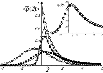
Figure 2: Rescaled counterion density $\left\langle\bar{\rho}(\tilde{z})\right\rangle=\left\langle\rho(\tilde{z})\right\rangle/2\pi\ell_{B}\sigma_{m}^{2}$ as a function of the rescaled distance $\tilde{z}=z/\mu$ from Monte Carlo simulations (data points) and asymptotic theory (solid lines). In the weak coupling limit ($\Xi=0.2$, solid squares), the membrane roughness is $\tilde{\xi}^{0}_{\bot}=1.211\,,0.3184\,,0$ and $\tilde{\xi}^{0}_{\|}=0.2483\,,0.2933\,,\infty$ from bottom to top. In the strong coupling limit ($\Xi=1000$, open triangles) we have $\tilde{\xi}^{0}_{\bot}=1.211\,,0.3184\,,0$ and $\tilde{\xi}^{0}_{\|}=17.2475\,,20.7458\,,\infty$ from bottom to top. Numerical errors are smaller then the symbol sizes. In all cases the membrane-ions are mobile and the packing fraction is $\zeta=0.028$. The inset compares profiles for $\Xi=0.2$, $\tilde{\xi}^{0}_{\bot}=0.3184$ for $\zeta=0.028$ (diamonds) and $\zeta=0.25$ (circles) for mobile membrane ions and results for $\Xi=0.2$, $\tilde{\xi}^{0}_{\bot}=1.211$, $\zeta=0.028$ for mobile (squares) and fixed (stars) membrane ions and $\Xi=1000$, $\tilde{\xi}^{0}_{\bot}=1.211$, $\zeta=0.028$ for mobile (triangle) and fixed (crosses) membrane ions.

In the analytics so far we used the bare membrane roughness $\tilde{\xi}^{0}_{\bot}$ without modification due to electrostatics. In Fig.3 we show the ratio of $\tilde{\xi}_{\bot}$, the membrane roughness measured in the MC simulation, and $\tilde{\xi}_{\bot}^{0}$, for the bare uncharged membrane, as a function of the coupling parameter $\Xi$ for two different surface fractions $\zeta$ (open symbols). The ratio is larger than unity, i.e. charges on the membrane increase the roughness. This short-range roughening, which allows membrane charges to increase their mutual distance and is thus not area-preserving, has to be distinguished from the electrostatic stiffening in the long-wavelength limit which has been predicted on the mean-field-level Winterhalter and Helfrich (1988); Lekkerkerker (1989); mitch . Local roughening corresponds to protrusion degrees of freedom of single lipids. Yet a distinct softening mechanism, effective at intermediate wavelengths, is due to electrostatic correlations effects phil ; me ; woon , which is missed by standard mean-field approaches. Experimentally, both membrane stiffening Rowat et al. (2004) and, for highly charged membranes, softening has been observed zemb . To distinguish effects due to membrane charges and counterions we calculate via exact enumeration and within harmonic approximation the membrane propagator $K_{mn}$ for a charged discrete membrane without counterions. The roughness ratio from this analytical calculations is shown as a solid line, and again cross-checked by MC simulations without counterions (filled symbols). The good agreement with the MC data containing counterions shows that the softening effect is mostly due to the repulsion of charges on the membrane itself. Experimentally, this short-scale roughening will show up in diffuse X-ray scattering data.

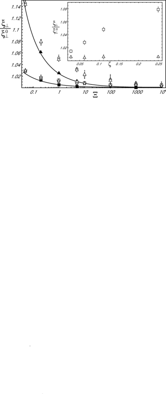
Figure 3: Ratio of simulated and bare roughness $\tilde{\xi}_{\bot}/\tilde{\xi}_{\bot}^{0}$ as a function of $\Xi$ for $\zeta=0.028$ and $\tilde{\xi}_{\bot}^{0}=0.3184$ (open squares) and $\tilde{\xi}_{\bot}^{0}=1.2111$ (open stars), $\zeta=0.25$ and $\tilde{\xi}_{\bot}^{0}=0.3184$ (open triangles) and $\tilde{\xi}_{\bot}^{0}=1.2111$ (open diamonds). The solid lines and solid symbols are analytical and MC results without counterions ($\zeta=0.028$ lower branch, $\zeta=0.25$ upper branch). The inset shows the ratio $\tilde{\xi}_{\bot}/\tilde{\xi}_{\bot}^{0}$ as a function of the packing fraction $\zeta$ for $\Xi=0.2$ (squares) and $\Xi=1000$ (triangles), $\tilde{\xi}_{\bot}^{0}=0.3184$ in both cases.

References

• (1)
• (2) Electrostatic Effects in Soft Matter and Biophysics, Holm C Kekicheff P Podgornik R (eds.), Kluwer Academic Publishers, Dordrecht (2001).
• (3) M.P Hentschel, M. Mischel, R.C. Oberthür, G. Büldt, FEBS Letters 193, 236 (1985).
• (4) J. Wang, M. Caffrey, M.J. Bedzyk, T.L. Penner, Langmuir 17, 3671 (2001).
• Richardsen et al. (1996) H. Richardsen, U. Vierl, G. Cevc, and W. Fenzl, Europhysics Letters 34, 543 (1996).
• (6) R. Das et al., Phys. Rev. Lett. 90, 188103 (2003).
• (7) T.E. Angelini, H. Liang, W. Wriggers, G.C.L. Wong, PNAS 100, 8634 (2003).
• (8) G. Brotond and T. Salditt, to be published.
• (9) R. Lipowsky, in The Structure and Dynamics of Membranes, edited by R. Lipowsky and E. Sackmann, Handbook on Biological Physics, Vol. 1, Elsevier, Amsterdam (1995).
• (10) A. G. Moreira and R. R. Netz, Eur. Phys. J. E 8 33, (2002)
• Moreira and Netz (2002a) A. G. Moreira and R. Netz, Europhys. Lett. 57, 911 (2002a); D.B. Lukatsky, S.A. Safran, A.W.C. Lau, and P. Pincus, ibid. 58, 785 (2002).
• (12) R.R. Netz and H. Orland, Eur. Phys. J. E 1 203 (2000).
• (13) R.R. Netz and H. Orland, Eur. Phys. J. E 11 301 (2003).
• Gouy (1910) G. Gouy, J. de Phys. IX, 457 (1910).
• Chapman (1913) D. L. Chapman, Phil. Mag. 25, 475 (1913).
• Winterhalter and Helfrich (1988) M. Winterhalter and W. Helfrich, J. Phys. Chem. 92, 6865 (1988).
• Lekkerkerker (1989) H. N. W. Lekkerkerker, Physica A 159, 319 (1989).
• (18) D.J. Mitchell and B.W. Ninham, Langmuir 5, 1121 (1989).
• (19) A.W.C. Lau and P. Pincus, Phys. Rev. Lett. 81, 1338 (1998).
• (20) R.R. Netz, Phys. Rev. E 64, 051401 (2001).
• (21) Y.W. Kim and W. Sung, Europhys. Lett. 58, 147 (2002).
• Rowat et al. (2004) A. C. Rowat, P. L. Hansen, and J. H. Ipsen, Europhysics Letters 67, 144 (2004).
• (23) B. Deme, M. Dubois, and T. Zemb, Langmuir 18, 1005 (2002).