Effective shear and extensional viscosities of concentrated disordered suspensions of rigid particles.

Abstract

We study effective shear viscosity $\mu^{\star}$ and effective extensional viscosity $\lambda^{\star}$ of concentrated non-colloidal suspensions of rigid spherical particles. The focus is on the spatially disordered arrays, but periodic arrays are considered as well. We use recently developed discrete network approximation techniques to obtain asymptotic formulas for $\mu^{\star}$ and $\lambda^{\star}$ as the typical inter-particle distance $\delta$ tends to zero, assuming that the fluid flow is governed by Stokes equations. For disordered arrays, the volume fraction alone does not determine the effective viscosity. Use of the network approximation allows us to study the dependence of $\mu^{\star}$ and $\lambda^{\star}$ on variable distances between neighboring particles in such arrays.

Our analysis, carried out for a two-dimensional model, can be characterized as global because it goes beyond the local analysis of flow between two particles and takes into account hydrodynamical interactions in the entire particle array. Previously, asymptotic formulas for $\mu^{\star}$ and $\lambda^{\star}$ were obtained via asymptotic analysis of lubrication effects in a single thin gap between two closely spaced particles. The principal conclusion in the paper is that, in general, asymptotic formulas for $\mu^{\star}$ and $\lambda^{\star}$ obtained by global analysis are different from the formulas obtained from local analysis. In particular, we show that the leading term in the asymptotics of $\mu^{\star}$ is of lower order than suggested by the local analysis (weak blow up), while the order of the leading term in the asymptotics of $\lambda^{\star}$ depends on the geometry of the particle array (either weak or strong blow up). We obtain geometric conditions on a random particle array under which the asymptotic order of $\lambda^{\star}$ coincides with the order of the local dissipation in a gap between two neighboring particles, and show that these conditions are generic. We also provide an example of a uniformly closely packed particle array for which the leading term in the asymptotics of $\lambda^{\star}$ degenerates (weak blow up).

1 Introduction

Concentrated suspensions are important in many industrial applications such as drilling, water-coal slurries transport, food processing, cosmetics and ceramics manufacture. In nature, flows of concentrated suspensions appear as mud slides, lava flows and soils liquefied by the earthquake-induced vibrations ([6], [7], [16]).

An asymptotic formula for the effective viscosity of a suspension of non-colloidal particles in a Newtonian fluid, derived in [9], is based on the local lubrication analysis of the energy dissipation rate in the narrow gap between a pair of nearly touching particles. The distance between two neighboring particles in a periodic array is the small parameter in the problem. For periodic arrays, this inter-particle distance is uniquely determined by the volume fraction of particles, so that the asymptotics of the effective viscosity is obtained as a function of the volume fraction $\phi$ that is close to the maximal packing volume fraction $\phi_{rcp}$. the asymptotics of the effective viscosity obtained in [9] has the form

$$A\epsilon^{-1}+O(\ln\epsilon),$$ (1.1)

as $\epsilon\to 0$, where $\epsilon=1-(\phi/\phi_{rcp})^{1/3}$. The formulas for effective viscosity of periodic suspensions in the whole space ${\bf R}^{3}$ (without boundary) subject to a prescribed linear flow, obtained in [11], also rely on the local lubrication analysis. Asymptotic representations for the components of the effective viscosity tensor calculated by [11] are of the form

$$A\epsilon^{-1}+B\ln\epsilon+O(1),$$ (1.2)

Recently, concentrated random suspensions were investigated numerically by [14] using accelerated Stokesian dynamics. It was observed that the behaviour of the effective high frequency dynamic shear viscosity of disordered suspensions can be accurately described by the asymptotic $B\ln\epsilon$, indicating degeneration of the leading term in the asymptotic expansions (1.2) (weak blow up). The authors of [14] also show that their results are in good agreement with available experimental data ([15], [17]). This suggests that for generic random suspensions, the asymptotics of the effective viscosity defined by the (properly normalized) global dissipation rate cannot be identified with the local dissipation rate in a single gap.

In this paper, we use the discrete network approximation proposed in [4] to study the asymptotics of the shear effective viscosity $\mu^{\star}$ and the extensional effective viscosity $\lambda^{\star}$ corresponding to general disordered particle arrays. For such arrays, the volume fraction alone is not sufficient for determining the effective viscosity. Therefore, instead of $\epsilon$, we use the inter-particle distance parameter $\delta$ that controls the distances $\delta_{ij}$ between neighboring particles.

The mathematical construction of [4] accounts for the long range hydrodynamical interactions between the particles, and provides an algorithm for calculation of the effective viscosity, which takes into account variable distances between neighboring particles in non-periodic arrays. Furthermore, in [4] it was observed that the leading term of the asymptotics may degenerate due to the external boundary conditions and geometry of the particle array, while in the scalar case ([5]) the order of the leading term is the same for all particle arrays that form a connected network. This paper is devoted to a detailed study of this degeneration phenomenon. In particular, we clarify the issue of weak versus strong blow up in the asymptotics of the effective viscosity.

The definition of the effective viscosity employed in this paper differs from the definition in [11]. Their definition is closely related to the definition of the effective material properties of periodic media in homogenization theory (see e.g. [3], [10]), where these properties are defined via analysis on a periodicity cell. Then these properties are determined by the properties of constituents and geometry of the periodic array, independently of the external boundary conditions and applied forces. Such properties are usually defined in the limit when particle size tends to zero while the number of particles approaches infinity.

Our definition is more directly linked to the viscometric measurements that necessarily involve boundary conditions. We assume that particles of a fixed size are placed in a bounded domain (apparatus), and the typical distance between the neighboring particles approaches zero. Thus, the total volume fraction of particles approaches the maximal packing fraction. In this case the effective viscosity will be influenced not just by the inter-particle interactions but also by the forces or velocities prescribed at the boundary of the apparatus. Since we work with linear models, $\mu^{\star}$ ($\lambda^{\star}$) are independent of the applied shear (extension) rate. However, we also show that the asymptotic order of the effective viscosities depends on the relation between the orientation of the velocity prescribed at the boundary, shape of the boundary, and orientations of the line segments connecting pairs of neighboring particles.

We present sufficient conditions for degeneration (weak blow up) and non-degeneration (strong blow up) of the leading term. We show that $\mu^{\star}$ always exhibits weak blow up, while local analysis alone predicts strong blow up. We also show that the asymptotic order of $\lambda^{\star}$ depends on the geometry of the particle array. In the paper, we define a broad class of arrays of particles for which the leading order term of $\lambda^{\star}$ does not degenerate. This situation is typical in the sense that for a generic array $\mu^{\star}$ and $\lambda^{\star}$ have vastly different values, and their ratio depends on the inter-particle distance, which indicates possible non-Newtonian behaviour of the effective fluid under the imposed boundary conditions. We also give an example of a closely packed particle array for which the leading term in the extensional viscosity degenerates.

2 Mathematical model

We consider a concentrated suspension of rigid, non-Brownian, neutrally buoyant particles in a viscous incompressible Newtonian fluid. In the two-dimensional model, the suspension occupies a domain $\Omega$ which is a square of side length two centered at the origin. The boundary of $\Omega$ is denoted by $\partial\Omega$. The upper and lower sides of $\partial\Omega$ are denoted by $\partial\Omega^{+}=\{{{\bf x}}:x_{2}=1\}$ and $\partial\Omega^{-}=\{{{\bf x}}:x_{2}=-1\}$, respectively. We also let ${\bf e}_{1},{\bf e_{2}}$ denote the Cartesian basis vectors parallel to the sides of $\partial\Omega$. The particles $D^{j}$, $j=1,2,\ldots,N$ are modelled as rigid disks with centers ${\bf x}^{j}$, placed in $\Omega$. For simplicity, we consider the monodisperse case, so that all particles have radius $a$. The part of $\Omega$ which is not occupied by particles is the fluid domain, denoted by $\Omega_{F}$.

The fluid at low Reynolds number is governed by Stokes equations

$$\mu\Delta{\bf v}-\nabla P=0,\;\;\;\;{\rm div}~{}{\bf v}=0,\;\;\;{\rm in}\;\Omega_{F}.$$ (2.1)

where $\mu$ is the fluid viscosity, $\bf v$ the velocity field, and $P$ is the pressure.

In this paper, we consider the external boundary conditions of the shear and extensional types. The shear type boundary conditions are given by

$${\bf v}=\left\{\begin{array}[]{cc}\gamma{\bf e}_{1}&{\rm on}~{}\partial\Omega^{+},\\ -\gamma{\bf e}_{1}&{\rm on}~{}\partial\Omega^{-},\\ \end{array}\right.$$ (2.2)

where $\gamma$ is a constant shear rate.

In the case of extensional boundary conditions the velocity is prescribed as

$${\bf v}=\left\{\begin{array}[]{cc}\varepsilon(-{\bf e}_{2}+x_{1}{\bf e}_{1})&{\rm on}~{}\partial\Omega^{+},\\ \varepsilon({\bf e}_{2}+x_{1}{\bf e}_{1})&{\rm on}~{}\partial\Omega^{-},\\ \end{array}\right.$$ (2.3)

where $\varepsilon$ is a constant extension rate. The two remaining (vertical) sides of $\partial\Omega$ are free surfaces, where the zero traction condition is prescribed.

To define particle velocities, we first recall that a rigid body moving in the plane defined by ${\bf e}_{1},{\bf e}_{2}$ has a velocity vector of the form

$${\bf v}^{j}({\bf x})={\bf T}^{j}+\omega^{j}{\bf e}_{3}\times({\bf x}-{\bf x}^{j}),\;\;\;{\bf x}\in D^{j},$$ (2.4)

where ${\bf e}_{3}$ is the unit vector perpendicular to the plane of motion. Therefore, if ${\bf r}=a{\bf e}_{1}+b{\bf e}_{2}$, then ${\bf e}_{3}\times{\bf r}=-b{\bf e}_{1}+a{\bf e}_{2}$. Equation (2.4) shows that the velocity of a particle $D^{j}$, $j=1,2,\ldots,N$ is completely determined by two parameters: a constant translational velocity vector ${\bf T}^{j}$ and a scalar angular velocity $\omega^{j}$. Both ${\bf T}^{j}$ and $\omega^{j}$ are unknown and must be determined in the course of solving the problem.

Since each rigid disk is in equilibrium, the total force and torque exerted on $D^{j}$ by the fluid must be zero, which provides the boundary conditions on the particle boundaries $\partial D^{j}$:

$$\int_{\partial D^{j}}\mbox{\boldmath$S$}{\bf n}^{j}\,ds={\bf 0}\;\;\hbox{and}\;\;\int_{\partial D^{j}}{\bf n}^{j}\times\mbox{\boldmath$S$}{\bf n}^{(j)}\,ds={\bf 0},\;\hbox{for}\;j=1,2\ldots N,,$$ (2.5)

where ${\bf n}^{j}$ is the exterior unit normal to $\partial D^{j}$, and

$$\mbox{\boldmath$S$}=2\mu\mbox{\boldmath$e$}({\bf v})-P\boldsymbol{I}.$$ (2.6)

In (2.6) and throughout the paper, $\mbox{\boldmath$e$}({\bf v})$ denotes the strain rate tensor defined by

$$\mbox{\boldmath$e$}({\bf v})=\frac{1}{2}(\nabla{\bf v}+\nabla{{\bf v}}^{T}),$$ (2.7)

the superscript $T$ stands for the transposed tensor, and $\boldsymbol{I}$ denotes the unit tensor.

Solving equation (2.1) with the boundary conditions (2.2) (or (2.3)) and (2.5) is equivalent to minimizing the functional

$$W_{\Omega_{F}}({\bf u})=\frac{\mu}{4}{\displaystyle\sum_{i,j=1}^{n}}{\displaystyle\int_{\Omega_{F}}}\left(\frac{\partial u_{i}({\bf x})}{\partial x_{j}}+\frac{\partial u_{j}({\bf x})}{\partial x_{i}}\right)^{2}d{\bf x},$$ (2.8)

over the function space ${\cal U}$ of admissible velocity fields ${\bf u}$. This space is a space of vector functions in $\Omega$ satisfying either (2.2) or (2.3), and such that

$${\bf u}={\displaystyle\sum_{j=1}^{n}}u_{j}\,{\bf e}_{j},~{}u_{j}\in H^{1}(\Omega_{F}),~{}j=1\ldots n,\;\hbox{div}\,{\bf u}=0,\;(\ref{p-vel})\,{\rm holds}.$$ (2.9)

Since the fluid velocity ${\bf v}$ is the minimizer of the variational principle (2.8)-(2.9), the energy dissipation rate $E$ in the fluid (defined in equation (3.2 below) can be written as

$$E=W_{\Omega_{F}}({\bf v})=\min_{{\bf u}\in{\cal U}}W_{\Omega_{F}}({\bf u}).$$ (2.10)

In next section we will see that calculation of the effective viscosities essentially amounts to calculation of $E$.

3 Effective shear and extensional viscosities.

3.1 Effective dissipation rates

We suppose that the suspension can be modelled on a macroscale by a single phase viscous fluid, called an effective fluid. The velocity field of the effective fluid is denoted by ${\bf v}^{0}$. The effective fluid is subject to the same external boundary conditions as the flow of the suspension.

We assume that the effective stress tensor ${\mbox{\boldmath$S$}}^{0}$ satisfies the constitutive equation of the form

$${\mbox{\boldmath$S$}}^{0}=F({\mbox{\boldmath$e$}}({\bf v}^{0})),$$ (3.1)

where $F$ is a symmetric tensor function that does not depend explicitly on ${\bf x}$. In this paper, we do not derive or postulate the precise from of the constitutive law for the effective fluid. Instead, we use the fundamental principle (going back to [8]), that viscous energy dissipation rate of the suspension must be equal to the dissipation rate of the effective homogeneous fluid. The dissipation rates are defined by

$$E=\int_{\Omega_{F}}{\mbox{\boldmath$S$}}\cdot{\mbox{\boldmath$e$}}({\bf v})d{{\bf x}}=2\mu\int_{\Omega_{F}}{\mbox{\boldmath$e$}}({\bf v})\cdot{\mbox{\boldmath$e$}}({\bf v})d{{\bf x}}$$ (3.2)

in the suspension, and

$$E^{0}=\int_{\Omega}{\mbox{\boldmath$S$}}^{0}\cdot{\mbox{\boldmath$e$}}({\bf v}^{0})d{\bf x},$$ (3.3)

in the effective fluid. In the equations (3.2), (3.3), ${\mbox{\boldmath$S$}}\cdot{\mbox{\boldmath$e$}}={\mbox{\boldmath$S$}}_{ij}{\mbox{\boldmath$e$}}_{ij}$ is the inner product of tensors.

For small particle volume fractions, ([8], [1]), this principle was further combined with the assumption that the effective fluid is Newtonian with a constant effective viscosity. However, for concentrated suspensions this assumption is not validated by rigorous mathematical derivation or experimental data and at present the problem of finding the effective constitutive law for such suspensions is still under investigation. Some experimental studies (e.g. [15], [17]) suggest that the effective fluid may be non-Newtonian. Our calculations of the effective viscosity suggest that non-Newtonian behavior is possible for irregular (non-periodic or random) suspensions.

We use the rheological definitions of shear and extensional viscosities as ratios of the corresponding components of the stress and strain rate tensors. To calculate the asymptotics of the two viscosities, we employ the network approximation introduced in ([4]). We analyze the network functional (discrete dissipation rate) introduced in [4] and show that the standard relation between two viscosities which holds for Newtonian fluids (see [13] ch. 9 for the 3D-case and Appendix A for 2D-case ) does not hold.

3.2 Shear viscosity

Suppose that a homogeneous effective fluid undergoes a steady shear flow with the shear rate $\gamma$. The velocity field ${\bf v}_{\it sh}$ satisfies the shear type boundary conditions (2.2). The effective shear viscosity is defined by (see (A.3))

$$\mu^{\star}=\frac{S^{0}_{12}}{\gamma}=2\frac{E^{0}}{\gamma^{2}|\Omega|},$$ (3.4)

where $S^{0}_{12}$ is the corresponding component of the effective stress tensor and $|\Omega|=\int_{\Omega}d{\bf x}$. Note that our definition of $F^{0}$ in (3.1) implies that $\mbox{\boldmath$S$}^{0}$ is constant when $\mbox{\boldmath$e$}({\bf v}^{0})$ is constant. Since $E=E^{0}$, the equivalent definition is

$$\mu^{\star}=2E\gamma^{-2}|\Omega|^{-1}=4\mu\gamma^{-2}|\Omega|^{-1}\int_{\Omega_{F}}{\mbox{\boldmath$e$}}({\bf v}_{\it sh})\cdot\mbox{\boldmath$e$}(\bf v_{\it sh})d{\bf x}$$ (3.5)

Thus the calculation of $\mu^{\star}$ amounts to evaluation of the total dissipation rate integral

$$E_{sh}=2\mu\int_{\Omega_{F}}{\mbox{\boldmath$e$}}({\bf v}_{\it sh})\cdot\mbox{\boldmath$e$}(\bf v_{\it sh}){\it d}{\bf x},$$ (3.6)

where $\bf v_{\it sh}$ solves (2.1)-(2.5).

3.3 Extensional viscosity

A steady extensional flow of the effective fluid is characterized by a constant extension rate $\varepsilon$. The velocity ${\bf v}^{0}_{\it ext}$ satisfies the extensional boundary conditions (2.3). The extensional viscosity (see, e.g. [13]. ch.9) may be defined by

$$\lambda^{\star}=\frac{S_{11}^{0}-S_{22}^{0}}{\varepsilon},$$ (3.7)

where $S_{11}^{0},S_{22}^{0}$ are components of the effective stress tensor. Since $E^{0}=\int_{\Omega}{\mbox{\boldmath$S$}}^{0}\cdot\mbox{\boldmath$e$}({\bf v})^{0}_{\it ext}d{\bf x}=(S_{11}^{0}-S_{22}^{0})\varepsilon|\Omega|$, the effective extensional viscosity can be defined in terms of the suspension dissipation rate $E$, as follows.

$$\lambda^{\star}=\frac{E}{\varepsilon^{2}|\Omega|}=2\mu\varepsilon^{-2}|\Omega|^{-1}\int_{\Omega_{F}}{\mbox{\boldmath$e$}}({\bf v}_{\it ext})\cdot{\mbox{\boldmath$e$}}({\bf v}_{\it ext})d{\bf x},$$ (3.8)

and calculation of $\lambda^{\star}$ again reduces to evaluation of the total dissipation rate (3.6) with ${\bf v}_{\it sh}$ replaced by ${\bf v}_{\it ext}$. In the remaining part of the paper we derive asymptotic formulas for the total dissipation rate under boundary conditions (2.2) and (2.3).

4 The Network

Let us consider an arbitrary distribution of circular particles (disks) $D^{i}$, whose centers are points ${\bf x}^{i}$ in $\Omega$, for $i=1,2,\ldots,N$. We suppose that $N$ is close to $N_{\hbox{max}}$, so that neighboring particles can be close to touching one another. The network consists of vertices ${\bf x}^{i}$ and edges. The edges connect only vertices that correspond to “ neighboring “ particles. Note that while for a periodic array the notion of a neighboring vertex (particle) is obvious, for non-periodic (e.g. random) arrays of particles it is not immediate. We introduce it via a Voronoi tessellation, which is a partition of a plane (or a planar domain) into the union of convex polygons $V_{i}$, called Voronoi cells, corresponding to the set of vertices ${\bf x}^{i}$. A Voronoi cell $V_{i}$ consists of all points in the plane which are closer to ${\bf x}^{i}$ than to any other vertex ${\bf x}^{j},j\neq i$.

The edges of $V_{i}$ can lie either on $\partial\Omega$ or in the interior of $\Omega$. On each face of $V_{i}$, that lies inside $\Omega$, $\mid{\bf x}-{\bf x}^{i}\mid=\mid{\bf x}-{\bf x}^{j}\mid,\;\hbox{for some}\;i\neq j.$

Definition 4.1

For each $i=1,2\ldots N$, define the index set ${\cal N}_{i}$ by

$${\cal N}_{i}=\left\{j\in\{1,2\ldots,N\},\;j\neq i,\;\hbox{such that}\;V_{i}\;\hbox{and}\;V_{j}\;\hbox{have a common edge}\right\}.$$

We call a particle $D^{j}$ a neighbor of $D^{i}$ if $j$ belongs to ${\cal N}_{i}$ that is the vertices ${\bf x}^{i}$ and ${\bf x}^{j}$ have a common edge in the Voronoi tessellation.

Note, that according to this definition, two particles are not neighbors if their Voronoi cells have a common vertex but do not share an edge.

The minimal distance between neighboring particles $D^{i}$ and $D^{j}$ is given by

$$\delta_{ij}=\mid{\bf x}^{i}-{\bf x}^{j}\mid-2a.$$ (4.1)

We call $\delta_{ij}$ inter-particle distances. If a disk $D^{i}$ is close to the external boundary $\partial\Omega$, we define the particle-boundary minimal distance $\delta_{i}$ by

$$\delta^{i}={\rm dist}({\bf x}^{i},\partial\Omega)-a.$$ (4.2)

To model the high concentration regime, we assume that $\delta_{ij}$ and $\delta_{i}$ satisfy

$$\delta_{ij}=\delta d_{ij},\;\;\;\;\;\delta_{i}=\delta d_{i},$$ (4.3)

where $\delta$ is a small parameter in the problem, and the scaled inter-particle distances $d_{ij},d_{i}$ satisfy

$$c\leq d_{ij}\leq 1,\;\;\;\;c\leq d_{i}\leq 1,$$ (4.4)

with a fixed positive $c$ independent of $i,j$.

Definition 4.2

The centers ${\bf x}^{i}$ of the particles $D^{i}$ are called the interior vertices of the network (graph) $\Gamma$, $i=1,2\ldots N$. The interior edges $b_{ij}$ of the network connect neighboring vertices ${\bf x}^{i}$ and ${\bf x}^{j}$. If a Voronoi cell $V_{i}$ has edges belonging to $\partial\Omega^{+}\bigcup\partial\Omega^{-}$, the corresponding ${\bf x}^{i}$ is called a near-boundary vertex. Each near-boundary vertex ${\bf x}^{i}$ is connected with $\partial\Omega^{\pm}$ by an exterior edge, which is a segment $\tilde{b}_{i}$ perpendicular to $\partial\Omega^{\pm}$. This segment intersects $\partial\Omega^{\pm}$ at an exterior vertex denoted by $\tilde{{\bf x}}^{(i)}$.

Finally, the network (graph) $\Gamma$ is the collection of all interior vertices, exterior vertices, and all the edges connecting these vertices.

The set of indices of the near-boundary vertices will be denoted by $I$, that is $i\in I$ if the vertex ${\bf x}^{i}$ is connected to $\partial\Omega$. Also, we write $i\in I^{+}(I^{-})$ if ${\bf x}^{i}$ is connected to $\partial\Omega^{+}(\partial\Omega^{-})$.

Note that $\Gamma$ is essentially the Delaunay graph dual to the Voronoi tessellation, and the above notions admit straightforward generalization to three dimensions.

5 Network approximation of the effective viscosity

5.1 Network equations

To define the network approximation, we first assign a translational velocity ${\bf T}^{i}$ and an angular velocity $\omega^{i}$ of a particle $D^{i}$ to the corresponding interior vertex ${\bf x}^{i}$. At the exterior vertices $\tilde{\bf x}^{i}$ we prescribe the velocity vector ${\bf g}$ which represents the boundary conditions (2.2) or (2.3).

For each pair of neighboring particles $D^{i}$ and $D^{j}$ we introduce a gap $\Pi_{ij}$ which represents a fluid region where lubrication effects are very strong as shown on Fig.1. The width $R_{ij}$ of such gap is independent of $\delta$. For technical reasons it is convenient to work with non-intersecting gaps. Since the maximal number of gaps adjacent to each particle is equal to the maximal coordination number (number of neighbors), K, we can choose $R_{ij}=KMa$, where $M$ is sufficiently small and fixed. The precise value of $M$ is not essential for our purposes.

Figure 1: A gap $\Pi_{ij}$ between the neighboring particles $D^{i}$ and $D^{j}$.

The orientation of each interior gap $\Pi_{ij}$ relative to a disk $D^{i}$ is specified by a unit vector

$${\bf q}^{ij}=\frac{{\bf x}^{i}-{\bf x}^{j}}{|{\bf x}^{i}-{\bf x}^{j}|}.$$ (5.1)

We also let ${\bf p}^{ij}$ be the unit vector obtained by rotating ${\bf q}^{ij}$ clockwise by $\pi/2$ (see Fig.2).

Boundary edges and corresponding gaps are oriented perpendicular to ${\bf e}_{1}$. This reflects the physical fact that the zone of the largest energy dissipation is located near the shortest line connecting ${\bf x}^{i}$ with the boundary. Therefore, ${\bf q}^{i}={\bf e_{2}}$, (respectively $-{\bf e}_{2}$), when $D^{i}$ is adjacent to $\partial\Omega^{+}$ (respectively $\partial\Omega^{-}$).

Figure 2: Assignment of ${\bf T}^{i},\omega^{i}$ and orientation of the gap between two neighboring particles.

Next, to each edge of the network we associate a dissipation rate $W^{ij}$ ($W^{i}$), calculated in the corresponding gap $\Pi_{ij}$ ($\Pi_{i}$). The calculation of the dissipation rates employs lubrication approximation in the gap. The velocity in the gap is decomposed into three velocities, representing the ”elementary” motions called spring motion, shear, and rotation (see Fig. 3). The total velocity field in a gap is the sum of these elementary velocities and a ”residual” velocity field, whose contribution to the gap dissipation rate is $O(1)$ as $\delta\to 0$. Lubrication approximations for each of the elementary velocities and estimates for the residual are obtained in [4] where more details can be found.

Figure 3: Three elementary motions. Arrows represent the boundary conditions.

Using approximations of the elementary velocities to calculate (up to the terms of order $O(1)$ as $\delta\to 0$) the dissipation rates in each gap we obtain

$$\begin{array}[]{ccc}W^{ij}&=&\delta^{-3/2}C^{ij}_{sp}\left[({\bf T}^{i}-{\bf T}^{j})\cdot{\bf q}^{ij}\right]^{2}+\\ &&\delta^{-1/2}C^{ij}_{sh}\left[({\bf T}^{i}-{\bf T}^{j})\cdot{\bf p}^{ij}+a{\omega}^{i}+a{\omega}^{j}\right]^{2}+\delta^{-1/2}C^{ij}_{rot}a^{2}(\omega^{i}-\omega^{j})^{2},\\ \end{array}$$ (5.2)

in the interior gaps $\Pi_{ij}$, and

$$W^{i}=\delta^{-3/2}C^{i}_{sp}\left[({\bf T}^{i}-{\bf g})\cdot{\bf q}^{i}\right]^{2}+\delta^{-1/2}C^{i}_{rot}a^{2}\left(2{\omega}^{i}\right)^{2}+\delta^{-1/2}C_{sh}^{i}\left[({\bf T}^{i}-{\bf g})\cdot{\bf p}^{i}+a{\omega}^{i}\right]^{2}$$ (5.3)

in the boundary gaps $\Pi_{i}$. The expressions for factors $C^{ij}_{sp},C^{ij}_{sh}$ and $C^{ij}_{rot}$ and $C^{i}_{sp},C^{i}_{sh},C^{i}_{rot}$ are calculated explicitly in [4]:

$$\begin{array}[]{ccccccc}C^{ij}_{sp}&=&\frac{3}{4}\pi\mu\big{(}\frac{a}{d_{ij}}\big{)}^{3/2}+\frac{27}{10}\pi\mu\big{(}\frac{a}{d_{ij}}\big{)}^{1/2},&&C^{i}_{sp}&=&\frac{3}{4}\pi\mu\big{(}\frac{a}{d_{i}}\big{)}^{3/2}+\frac{27}{10}\pi\mu\big{(}\frac{a}{d_{i}}\big{)}^{1/2},\\ C^{ij}_{sh}&=&\frac{1}{2}\pi\mu\big{(}\frac{a}{d_{ij}}\big{)}^{1/2},&&C^{i}_{sh}&=&\frac{1}{2}\pi\mu\big{(}\frac{a}{d_{i}}\big{)}^{1/2},\\ C^{ij}_{rot}&=&\frac{9}{16}\pi\mu\big{(}\frac{a}{d_{ij}}\big{)}^{1/2}.&&C^{i}_{rot}&=&\frac{9}{16}\pi\mu\big{(}\frac{a}{d_{i}}\big{)}^{1/2}.\\ \end{array}$$ (5.4)

In the formulas (5.4), $d_{ij},d_{i}$ are the scaled inter-particle distances defined in (4.4).

The sum of the local dissipation rates $W^{ij},W^{i}$ is a quadratic form

$$\begin{array}[]{lll}Q&=&\sum_{\Pi_{ij}}W^{ij}+\sum_{\Pi_{i}}W^{i}\\ &=&{\displaystyle\sum_{i=1}^{N}}{\displaystyle\sum_{{\tiny\begin{array}[]{c}j\in{\cal N}_{i}\\ j<i\end{array}}}}\left\{\delta^{-3/2}C^{ij}_{sp}\left[({\bf T}^{i}-{\bf T}^{j})\cdot{\bf q}^{ij}\right]^{2}+\delta^{-1/2}C^{ij}_{sh}\left[({\bf T}^{i}-{\bf T}^{j})\cdot{\bf p}^{ij}+a{\omega}^{i}+a{\omega}^{j}\right]^{2}\right.\\ &&+\left.\delta^{-1/2}C^{ij}_{rot}a^{2}\left({\omega}^{i}-{\omega}^{j}\right)^{2}\right\}+{\displaystyle\sum_{i\in I}}\left\{\delta^{-3/2}C^{i}_{sp}\left[({\bf T}^{i}-{\bf g})\cdot{\bf q}^{i}\right]^{2}+\delta^{-1/2}C^{i}_{rot}a^{2}\left(2{\omega}^{i}\right)^{2}\right.\\ &&+\left.\delta^{-1/2}C_{sh}^{i}\left[({\bf T}^{i}-{\bf g})\cdot{\bf p}^{i}+a{\omega}^{i}\right]^{2}\right\},\end{array}$$ (5.5)

where $I$ denotes the set of indices of the near-boundary vertices defined in Section 4.

The form $Q$ is the discrete network approximation of the functional $W_{\Omega_{F}}$ in the variational principle (2.8). The main idea of the network approximation is that the most of the energy is dissipated in the gaps $\Pi_{ij},\Pi_{i}$, so that

$$E=E_{net}+O(1),\;\;\;\;{\rm as}\;\delta\to 0.$$ (5.6)

The discrete dissipation rate $E_{net}$ in (5.6) is defined by

$$E_{net}=\min_{{\bf T}^{i},\omega^{i}}Q=Q({\bf T}_{min}^{1},{\bf T}^{2}_{min},...{\bf T}^{N}_{min},{\omega}^{1}_{min},...{\omega}^{N}_{min}),$$ (5.7)

where the vectors ${\bf T}^{i}_{min},i=1,2,\ldots,N$ and scalars ${\omega}^{i},i=1,2,\ldots,N$ minimize $Q$ in (5.5). The minimum in (5.7) is taken over all possible collections of ${\bf T}^{i},\omega^{i}$.

It is well known that solving the minimization problem for $Q$ is equivalent to solving the linear system (Euler-Lagrange equations), which is obtained by equating the gradient of $Q$ to zero. Setting to zero partial derivatives with respect to $T^{i}_{l},l=1,2$ we obtain

$$\sum_{j\in{\cal N}_{i}}\left\{\delta^{-3/2}C^{ij}_{sp}\left[({\bf T}^{i}-{\bf T}^{j})\cdot{\bf{q}}^{ij}\right]{\bf{q}}^{ij}\right\}+\hskip 103.85237pt$$

$$\sum_{j\in{\cal N}_{i}}\left\{\delta^{-1/2}C^{ij}_{sh}\left[({\bf T}^{i}-{\bf T}^{j})\cdot{\bf{p}}^{ij}+a{\omega}^{i}+a{\omega}^{j}\right]{\bf{p}}^{ij}\right\}+{\bf B}^{i}={\bf F}^{i},~{}~{}$$ (5.8)

for each $i=1,2,...,N$, where

$${\bf B}^{i} = \left\{\begin{array}[]{l}\delta^{-3/2}C^{i}_{sp}({\bf T}^{i}\cdot{\bf q}^{i}){\bf q}^{i}+\delta^{-1/2}C^{i}_{sh}\left[{\bf T}^{i}\cdot{\bf p}^{i}+a{\omega}^{i}\right]{\bf p}^{i},~{}~{}\mbox{if}~{}i\in I\\ {\bf 0}~{}~{}\mbox{otherwise},\end{array}\right.$$ (5.11)

$${\bf F}^{i} = \left\{\begin{array}[]{l}\delta^{-3/2}C^{i}_{sp}({\bf g}\cdot{\bf q}^{i}){\bf q}^{i}+\delta^{-1/2}C^{i}_{sh}({\bf g}\cdot{\bf p}^{i}){\bf p}^{i},~{}~{}\mbox{if}~{}i\in I\\ {\bf 0}~{}~{}\mbox{otherwise},\end{array}\right.$$ (5.15)

Next, equating the partial derivatives $\frac{\partial Q}{\partial\omega^{i}}$ to zero we obtain

$$\sum_{j\in{\cal N}_{i}}\left\{\delta^{-1/2}C^{ij}_{sh}\left[({\bf T}^{i}-{\bf T}^{j})\cdot{\bf{p}}^{ij}+a{\omega}^{i}+a{\omega}^{j}\right]\right\}+$$

$$\sum_{j\in{\cal N}_{i}}\left\{\delta^{-1/2}C^{ij}_{rot}\left({\omega}^{i}-{\omega}^{j}\right)\right\}+{\cal B}^{i}={\cal M}^{i},\hskip 42.67912pt$$ (5.17)

for all $i=1,\ldots,N$, where

$${\cal B}^{i} = \left\{\begin{array}[]{l}\delta^{-1/2}C_{sh}^{i}\left({\bf T}^{i}\cdot{\bf p}^{i}+a{\omega}^{i}\right)+4\delta^{-1/2}C^{i}_{rot}{\omega}^{i},~{}~{}\mbox{if}~{}i\in I,\\ 0~{}~{}\mbox{otherwise}.\end{array}\right.$$ (5.20)

$${\cal M}^{i} = \left\{\begin{array}[]{l}\delta^{-1/2}C_{sh}^{i}\left({\bf g}\cdot{\bf p}^{i}\right)~{}~{}\mbox{if}~{}i\in I,\\ 0~{}~{}\mbox{otherwise}.\end{array}\right.\hskip 113.81102pt$$ (5.23)

Equations (5.8) and (5.17) are, respectively, the equations of force and torque balance of the particles, and the minimization in (5.5) ensures that the rigid body translational and angular velocities are chosen in such a way that the suspension is in mechanical equilibrium. Note also that (5.8) is a system of $2N$ equations, and (5.17) is a system of $N$ equations. Together they form $3N$ equations for $3N$ unknowns $({\bf T}^{i},\omega^{i})$. The coefficients and right hand side of (5.8) are of order $\delta^{-3/2}$ and $\delta^{-1/2}$ while all the coefficients in (5.17) are of order $\delta^{-1/2}$. When all ${\bf T}^{i}$ are zero (no translations), the remaining terms are of order $\delta^{-1/2}$, but in the case $\omega^{i}=0,i=1,2,\ldots,N$ (no rotations), the remaining equations contain terms of order $\delta^{-3/2}$. This reflects the well known fact that the contributions from local translational spring motions are stronger than the contributions from rotational and other translational motions. Keeping only spring translations we obtain the truncated (leading order) discrete dissipation functional

$$\delta^{-3/2}\widehat{Q}=\delta^{-3/2}\displaystyle{\left[\frac{1}{2}\sum_{i=1}^{N}\sum_{j\in{\cal N}_{i}}C^{ij}_{sp}(({\bf T}^{i}-{\bf T}^{j})\cdot{\bf q}^{ij})^{2}+\sum_{i\in I}C_{sp}^{i}(({\bf T}^{i}-{\bf g})\cdot{\bf q}^{i})^{2}\right].}$$ (5.24)

Then $Q$ can be decomposed as follows.

$$Q=\delta^{-3/2}\widehat{Q}+\delta^{-1/2}Q^{\prime},$$ (5.25)

where the coefficients of the forms $\widehat{Q}$ and $Q^{\prime}$ do not depend on $\delta$.

We next show that the total discrete dissipation rate $E_{net}$ can be estimated by the truncated dissipation rate obtained by minimizing $\widehat{Q}$. Let $\widehat{{\bf T}^{i}},i=1,2,\ldots,N$ denote the translational velocities which minimize $\widehat{Q}$ ( they are clearly independent of $\delta$). Since $Q^{\prime}$ in (5.25) is non-negative,

$$\delta^{-3/2}\widehat{Q}(\widehat{{\bf T}^{i}})\leq\delta^{-3/2}\widehat{Q}({\bf T}^{i}_{min},{\omega}^{i}_{min})\leq E_{net}=\hskip 28.45274pt$$

$$Q({\bf T}^{i}_{min},\omega^{i}_{\min})\leq\delta^{-3/2}\widehat{Q}(\widehat{{\bf T}^{i}})+\delta^{-1/2}Q^{\prime}(\widehat{{\bf T}^{i}},{\omega}^{i}=0).$$ (5.26)

Since $Q^{\prime}(\widehat{{\bf T}^{i}},{\omega}^{i}=0)\leq C$ with $C$ independent of $\delta$ as $\delta\to 0$, (5.26) implies

$$E_{net}=\delta^{-3/2}\widehat{E}+O(\delta^{-1/2}),\;\;\;\;{\rm as}~{}\delta\to 0,$$ (5.27)

where

$$\widehat{E}=\widehat{Q}(\widehat{{\bf T}^{i}})={\displaystyle\min_{{\tiny{\bf T}^{1},\ldots{\bf T}^{N}}}\widehat{Q}({\bf T}^{1},\ldots{\bf T}^{N}}).$$ (5.28)

This equation enables one to calculate the leading term in the asymptotics of the effective viscosity by solving a simplified minimization problem involving only the translational particle velocities. However, this algorithm is useful only when

$$\widehat{E}>0,$$ (5.29)

because in this case the leading term in the asymptotics of the dissipation rate is of order $\delta^{-3/2}$. If $\min\widehat{Q}=0$, the leading term degenerates, and the rate of blow up in (5.28) is at most $\delta^{-1/2}$.

Minimization of the truncated quadratic form $\widehat{Q}$ corresponds to solving the truncated linear system of the Euler-Lagrange equations

$$\sum_{j\in{\cal N}_{i}}\big{[}C^{ij}_{sp}(\widehat{{\bf T}}^{i}-\widehat{{\bf T}}^{j})\cdot{\bf{q}}^{ij}{\bf{q}}^{ij}\big{]}+{\bf B}({\widehat{{\bf T}^{i}}})={\bf R}^{i},\;\;\;\;i=1,2,\ldots,N,$$ (5.30)

where

$${\bf B}(\widehat{{\bf T}^{i}})=\begin{cases}C_{sp}^{i}(\widehat{{\bf T}^{i}}\cdot{\bf q}^{i}){\bf q}^{i},\;\;\;\;{\rm when}~{}i\in I&\\ 0\;\;\;\;\;\;{\rm otherwise}.&\\ \end{cases}$$ (5.31)

The right hand side vectors ${\bf R}^{i}$ represent external boundary conditions:

$${\bf R}^{i}=\begin{cases}C_{sp}^{i}({\bf g}\cdot{\bf q}^{i}){\bf q}^{i},\;\;\;\;{\rm when}~{}i\in I&\\ 0\;\;\;\;\;\;{\rm otherwise}.&\\ \end{cases}$$ (5.32)

To better see the structure of the functional $\widehat{Q}$ and the system (5.30) it is convenient to rewrite them in a compact form as

$$\hat{Q}({\bf z})=\frac{1}{2}A{\bf z}\cdot{\bf z}-{\bf f}\cdot{\bf z}+r,$$ (5.33)

and

$$A{\bf z}={\bf f},$$ (5.34)

where ${\bf z}$ is the particle velocity vector, and ${\bf f}$ is the vector of discretized boundary conditions. The vectors ${\bf z},{\bf f}\in{\bf R}^{2N}$ are defined by

$${\bf z}=\left(\begin{array}[]{c}T^{1}_{1}\\ T^{1}_{2}\\ T^{2}_{1}\\ T^{2}_{2}\\ ...\\ T^{N}_{1}\\ T^{N}_{2}\\ \end{array}\right),\;\;\;\;\;\;\;{\rm and}\;\;\;\;\;\;\;{\bf f}=2\left(\begin{array}[]{c}R^{1}_{1}\\ R^{1}_{2}\\ R^{2}_{1}\\ R^{2}_{2}\\ ...\\ R^{N}_{1}\\ R^{N}_{2},\\ \end{array}\right).$$ (5.35)

The fixed scalar $r$ equals $\tilde{\bf f}\cdot{\bf f}$ where components of $\tilde{\bf f}$ are defined by the components of ${\bf f}$, as follows.

$$\tilde{f}_{2k-1}=\frac{1}{4C_{sp}^{k}}f_{2k-1},\;\;\;\;\tilde{f}_{2k}=\frac{1}{4C_{sp}^{k}}f_{2k}\;\;\;\;\;\;k=1,2,\ldots,N.$$

The matrix $A$ in (5.33) is symmetric and non-negative definite. Its entries are determined by the scaled inter-particle distances $d_{ij}$, particle radius $a$ and vectors ${\bf q}^{ij},{\bf q}^{i}$ defined by (5.1). The vector ${\bf f}$ and the scalar $r$ in (5.33) are determined by the boundary conditions on $\partial\Omega^{+},\partial\Omega^{-}$ (extensional or shear). The linear term ${\bf f}\cdot{\bf z}$ depends on the translational velocities of the particles located near $\partial\Omega^{+}$ or $\partial\Omega^{-}$.

To the leading order in $\delta$, the effective viscosity is determined by the discrete dissipation rate $\delta^{-3/2}\widehat{E}$ where $\widehat{E}$ is the minimum of $\widehat{Q}$. Thus the qualitative behaviour of the effective viscosity is determined by solving (5.34). We now sketch the issues which arise in computing the leading term of the effective viscosity. First, in the case of shear viscosity, ${\bf f}=0$, which means that the shear boundary conditions do not contribute to the strong blow up. This results in the weak blow up of $\mu^{\star}$ (see section 6). In case of extensional conditions, ${\bf f}\neq 0$, which means that the right hand side of the full network equations (5.8) contains terms of order $\delta^{-3/2}$. In this case, calculation of the leading term is impeded by the fact that the matrix $A$ is not invertible. Indeed, from (5.24) it is clear that the value of $\widehat{Q}$ does not change when all vectors ${\bf T}^{i},i=1,2,\ldots,N$ are replaced by ${\bf T}^{i}+t{\bf e}_{1}$ (horizontal translation by $t{\bf e}_{1}$, $t$ arbitrary real). This is not surprising, because the functional $\widehat{Q}$ is invariant under horizontal translation of ${\bf T}^{i}$. The invariance is due to the vertical orientation of the boundary gaps explained in section 5.1. Note that this is not equivalent to translation of a coordinate system, since ${\bf g}$ is not changed. Translational invariance of $\widehat{Q}$ implies that any ${\bf z}^{*}$ that solves the non-homogeneous system (5.34) produces other solutions of the form ${\bf z}^{*}+t{\bf w}_{0},$ where $t$ is arbitrary real, and

$${\bf w}_{0}=(1,0,1,0,\ldots,1,0)^{T}.$$ (5.36)

This means that vectors of the form $t{\bf w}_{0}$ solve the homogeneous system

$$A{\bf z}={\bf 0}.$$ (5.37)

Because of the above mentioned invariance of the functional $\widehat{Q}$, the leading term in the asymptotics of effective viscosity will be uniquely defined, unless (5.37) has some other nontrivial solutions. Therefore, it makes sense to look for conditions on the network which would guarantee that every solution of the homogeneous system is of the form $t{\bf w}_{0}$. Then the non-homogeneous system (5.34) would be uniquely solvable up to horizontal translation. In Section 7.3 we show that for a typical random distribution of particles this is indeed the case.

The last issue concerns the validity of the estimate (5.29). The functional $\widehat{Q}$ is non-negative, but it may be zero. When (5.29) holds, local lubrication analysis provides the correct order of the leading term in the asymptotics of the extensional effective viscosity ($\delta^{-3/2}$ in dimension two and $\delta^{-1}$ in dimension three). If (5.29) does not hold, that is,

$$\min\widehat{Q}=0,$$ (5.38)

then the leading term in dimension two is of order $\delta^{-1/2}$, ($\ln(1/\delta)$ in dimension three).

Whether or not the estimate (5.29) holds, depends on the geometry of the particle array as well as the boundary conditions on $\partial\Omega^{+}$ and $\partial\Omega^{-}$. In section 7.4 we show that in the case of extensional boundary conditions, (5.29) holds for generic arrays, and thus the leading term in the asymptotic of $E_{net}$ ( and extensional effective viscosity $\lambda^{*}$, see (3.8)) is of the order $\delta^{-3/2}$. However, there exist special arrays for which the extensional effective viscosity is of order $\delta^{-1/2}$. An example of such an array is presented in section 7.5.

6 Effective shear viscosity

In this Section we show that in dimension two, the asymptotic order of the shear effective viscosity $\mu^{\star}$ is $\delta^{-1/2}$, while the local lubrication analysis predicts the rate $\delta^{-3/2}$. In three dimensions, $\delta^{-1/2}$ and $\delta^{-3/2}$ should be replaced by, respectively, $\ln\delta$ and $\delta^{-1}$ (see [4]). The local analysis in three dimensions predicts that the asymptotics of the shear effective viscosity $\mu^{\star}$ (see (3.5)) should be of order $\delta^{-1}$, but numerical simulations in [14] and experimental results in [15] and [17] show that random suspensions in shear flow have effective viscosity of order $\ln\delta$. Our estimate $\mu^{\star}=O(\delta^{-1/2})$ is therefore in agreement with the three-dimensional results in [14], up to the difference in the dimension of the space.

The decrease in the asymptotic order of $\mu^{\star}$ is a global phenomenon, which shows that the local analysis could be misleading, and analysis of the entire particle array leads to qualitatively different results. This fact can be explained as follows. The ”strong” blow up rate ($\delta^{-1}$ in three dimensions and $\delta^{-3/2}$ in two dimensions) is obtained using classical lubrication techniques applied to two particles $D^{i},D^{j}$ whose translational and angular velocities ${\bf T}^{i},{\bf T}^{j},\omega^{i},\omega^{j}$ are independent of $\delta$. However, the network analysis of the ensemble of particles, interacting with each other and with the external boundary, shows that the above velocities may depend on $\delta$. In the case of shear boundary conditions, the right hand side of the network equations (5.8), (5.17) is of order $\delta^{-1/2}$, whereas the matrix of the network equations is of order $\delta^{-3/2}$. The solution of the network equations is thus small (of order $\delta$) which makes local and global dissipation rates small.

When the boundary conditions are given by (2.2), the vectors ${\bf R}^{i}$ in (5.32) are zero (since ${\bf q}^{i}\cdot{\bf e}_{1}=0$ for all $i=1,2,\ldots,N$). Consequently, the right hand side ${\bf f}$ in (5.34) is zero. The functional $\widehat{Q}$ reduces to $A{\bf z}\cdot{\bf z}$ which is clearly zero for every solution of the homogeneous system $A{\bf z}=0$. Since ${\bf z}=0$ is an admissible trial vector for $\widehat{Q}$, $\widehat{E}=\min\widehat{Q}=0$, and from (5.27) we obtain

$$\mu^{\star}=CE_{net}=O(\delta^{-1/2}),$$ (6.1)

where $C=2\gamma^{-2}|\Omega|^{-1}$ (see (3.5)). The same conclusion can be obtained by directly estimating the minimum of the form $Q$. Consider first the shear boundary conditions (2.2) with $\gamma=1$ and a simple example of a two-disk network on Fig. 4.

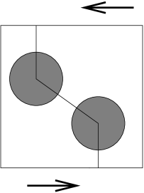
Figure 4: A two-disk network with shear boundary conditions.

The functional $Q$ for this example has the form

$$\begin{array}[]{ccc}Q&=&\delta^{-3/2}\left\{C_{sp}^{12}\left[({\bf T}^{1}-{\bf T}^{2})\cdot{\bf q}^{12}\right]^{2}+C_{sp}^{1}\left[({\bf T}^{1}-{\bf e}_{1})\cdot{\bf e}_{2}\right]^{2}+C_{sp}^{2}\left[({\bf T}^{2}+{\bf e}_{1})\cdot{\bf e}_{2}\right]^{2}\right\}\\ &&+\delta^{-1/2}\left\{C_{sh}^{12}\left[({\bf T}^{1}-{\bf T}^{2})\cdot{\bf p}^{12}+a\omega_{1}+a\omega_{2}\right]^{2}+C_{rot}^{12}a^{2}(\omega_{1}-\omega_{2})^{2}\right\}\\ &&+\delta^{-1/2}\left\{C_{sh}^{1}\left[({\bf T}^{1}-{\bf e}_{1})\cdot{\bf e}_{1}+a\omega_{1}\right]^{2}+C_{sh}^{2}\left[({\bf T}^{2}+{\bf e}_{1})\cdot{\bf e}_{1}+a\omega_{2}\right]^{2}\right\}\\ &&+\delta^{-1/2}\left\{4C_{rot}^{1}a^{2}{\omega_{1}}^{2}+4C_{rot}^{2}a^{2}{\omega_{2}}^{2}\right\}.\end{array}$$ (6.2)

The dissipation rate $E$ is the minimum of $Q$. Hence, for any collection ${\bf T}^{1},{\bf T}^{2},\omega_{1},\omega_{2}$, we have $E\leq Q({\bf T}^{1},{\bf T}^{2},\omega_{1},\omega_{2})$. In particular, choosing ${\bf T}^{1}={\bf T}^{2}={\bf 0},\omega_{1}=\omega_{2}=0$ in (6.2) we obtain

$$E\leq\delta^{-1/2}(C^{1}_{sh}+C^{2}_{sh})$$

Since $C_{sh}^{1},C_{sh}^{2}$ are independent of $\delta$, the blow up rate of $E$ is at most $\delta^{-1/2}$.

Next, consider the general case. Since for shear boundary condition ${\bf g}\bot{\bf q}^{i}$ for all $i\in I$, we obtain

$$\begin{array}[]{lll}Q&=&{\displaystyle\sum_{i=1}^{N}}{\displaystyle\sum_{{\tiny\begin{array}[]{c}j\in{\cal N}_{i}\\ j<i\end{array}}}}\left\{\delta^{-3/2}C^{ij}_{sp}\left[({\bf T}^{i}-{\bf T}^{j})\cdot{\bf q}^{ij}\right]^{2}\right\}+\\ &&{\displaystyle\sum_{i=1}^{N}}{\displaystyle\sum_{{\tiny\begin{array}[]{c}j\in{\cal N}_{i}\\ j<i\end{array}}}}\left\{\delta^{-1/2}C^{ij}_{sh}\left[({\bf T}^{i}-{\bf T}^{j})\cdot{\bf p}^{ij}+a{\omega}^{i}+a{\omega}^{j}\right]^{2}\right.+\left.\delta^{-1/2}C^{ij}_{rot}a^{2}\left({\omega}^{i}-{\omega}^{j}\right)^{2}\right\}+\\ &&{\displaystyle\sum_{i\in I}}\left\{\delta^{-3/2}C^{i}_{sp}\left[{\bf T}^{i}\cdot{\bf q}^{i}\right]^{2}+\delta^{-1/2}C^{i}_{rot}a^{2}\left(2{\omega}^{i}\right)^{2}\right\}+\\ &&{\displaystyle\sum_{i\in I}}\left\{\delta^{-1/2}C_{sh}^{i}\left[({\bf T}^{i}\cdot{\bf p}^{i}-{\bf g}\cdot{\bf p}^{i}+a{\omega}^{i}\right]^{2}\right\},\end{array}$$ (6.3)

Choosing the trial vectors ${\bf T}^{i}$ as ${\bf T}^{i}=0,i=1,2,\ldots,N$ and $\omega^{i}=0$, $i=1,2,\dots,N$ we obtain

$$E_{net}=\min Q\leq Q({\bf T}^{i}={\bf 0},\omega^{i}=0)=\delta^{-1/2}\sum_{i\in I}C_{sh}^{i}({\bf g}\cdot{\bf p}^{i})^{2}=\gamma^{2}\delta^{-1/2}\sum_{i\in I}C_{sh}^{i}.$$ (6.4)

where we used the shear boundary conditions (2.2). The sum in the right hand side of (6.4) is independent of $\delta$ and the shear rate $\gamma$. This estimate shows that under the boundary conditions (2.2), the effective viscosity blows up as $\delta^{-1/2}$ at most. More precisely, we have the following
Conclusion. Effective shear viscosity of a concentrated suspension has the blow up rate $\delta^{-1/2}$ in two dimensions, that is

$$\mu^{\star}\leq C\delta^{-1/2}\;\;\;{\rm as}~{}\delta\to 0,$$

with $C$ independent of $\delta,\gamma$.

7 Extensional effective viscosity

7.1 Simplification of boundary conditions and outline of the method

In this Section we show that for the extensional boundary conditions, the leading term in the asymptotics of the dissipation rate $E$ from (5.27) may or may not be zero depending on the geometry of a particle array, that is, the leading term in the asymptotics of the effective extensional viscosity is either of order $\delta^{-3/2}$ (strong blow up) or $\delta^{-1/2}$ (weak blow up). We provide two geometric conditions on the network graph which ensure strong blow up.

In a planar steady extensional flow of the effective fluid, the rate of strain tensor is

$$e({\bf v}^{0})=\left(\begin{array}[]{cc}\epsilon&0\\ 0&-\epsilon\\ \end{array}\right),$$ (7.1)

where $\epsilon$ denotes a constant extension rate. The corresponding velocity field is of the form

$${\bf v}^{0}=(\epsilon x_{1},-\epsilon x_{2})^{T},$$ (7.2)

which gives the boundary conditions

$${\bf v}^{0}=\begin{cases}(\epsilon x_{1},-\epsilon)^{T},\;\;{\rm when}\;x_{2}=1\;\;({\rm on}\;\partial\Omega^{+}),&\\ (\epsilon x_{1},\epsilon)^{T},\;\;{\rm when}\;x_{2}=-1\;\;({\rm on}\;\partial\Omega^{-}).&\\ \end{cases}$$ (7.3)

We decompose ${\bf v}^{0}$ as

$${\bf v}^{0}={\bf v}^{0}_{vc}+{\bf v}^{0}_{ge},$$ (7.4)

where ${\bf v}^{0}_{vc}$ is a vertical contraction velocity satisfying

$${\bf v}^{0}_{vc}={\bf g}_{vc}=\begin{cases}-\epsilon{\bf e}_{2}~{}~{}~{}{\rm on}~{}\partial\Omega^{+},&\\ \;\;\;\epsilon{\bf e}_{2}~{}~{}~{}{\rm on}~{}\partial\Omega^{-},&\\ \end{cases}$$ (7.5)

and ${\bf v}^{0}_{ge}$ is the horizontal extension velocity field with the boundary conditions given by

$${\bf v}^{0}_{ge}={\bf g}_{ge}\begin{cases}\epsilon x_{1}{\bf e}_{1}~{}~{}~{}{\rm on}~{}\partial\Omega^{+},&\\ \epsilon x_{1}{\bf e}_{1}~{}~{}{\rm on}~{}\partial\Omega^{-}.&\\ \end{cases}$$ (7.6)

Since

$${\bf g}={\bf g}_{vc}+{\bf g}_{ge},$$ (7.7)

and ${\bf g}_{ge}\bot{\bf q}^{i},i\in I$, the value of $\widehat{Q}$ in (5.24) does not change when ${\bf g}$ in (5.24) is replaced by ${\bf g}_{vc}$. Hence,

$$Q({\bf T}^{i},\omega^{i},{\bf g})=\delta^{-3/2}\widehat{Q}({\bf T}^{i},{\bf g}_{vc})+\delta^{-1/2}Q^{\prime}({\bf T}^{i},\omega^{i},{\bf g}_{vc}+{\bf g}_{ge}),$$ (7.8)

To determine the rate of blow up of the dissipation rate, we need to analyze the minimizers of $\widehat{Q}({\bf T}^{i},{\bf g}_{vc})$. The estimate (5.27) implies that the second term in the right hand side of (7.8) is of order $\delta^{-1/2}$ (at most). Since $\widehat{Q}$ is independent of $\delta$, its minimizing vectors $\widehat{\bf T}^{i}$ are also $\delta$-independent. Consequently, the blow up rate of the dissipation depends on whether the minimum of $\widehat{Q}({\bf T}^{i},{\bf g}_{vc})$ is positive. If it is, the extensional effective viscosity $\lambda^{\star}$ is of order $\delta^{-3/2}$, otherwise $\lambda^{\star}$ grows no faster than $\delta^{-1/2}$. Which type of behavior occurs, depends on the validity of the estimate (5.29). As mentioned in section 5, (5.29) may fail for certain particle arrays. In this section we provide geometric conditions which insure positivity of $\min\widehat{Q}$, and give examples of networks for which this minimum is zero. The principal conclusion here is that extensional viscosity of suspensions with a comparable volume fraction of particles may vary by an order of magnitude in the inter-particle distance, depending on the geometry of a particle array.

Our method of analysis is based on the following simple observation. The form $\widehat{Q}({\bf T}^{i},{\bf g}_{vc})$ is a sum of non-negative terms, namely

$$\widehat{Q}({\bf T}^{i},{\bf g}_{vc})=\displaystyle{\frac{1}{2}\sum_{i=1}^{N}\sum_{j\in{\cal N}_{i}}C^{ij}_{sp}(({\bf T}^{i}-{\bf T}^{j})\cdot{\bf q}^{ij})^{2}+\sum_{i\in I}C_{sp}^{i}(({\bf T}^{i}-{\bf g}_{vc})\cdot{\bf q}^{i})^{2}.}$$ (7.9)

This shows that $\min\widehat{Q}({\bf T}^{i},{\bf g}_{vc})=0$ if and only if the minimizing vectors ${{\bf T}^{i}},i=1,2,\dots,N$ satisfy the system of equations

$$\begin{array}[]{c}({\bf T}^{i}-{\bf T}^{j})\cdot{\bf q}^{ij}=0,\;\;\;\;\;i=1,2..N,j\in{\cal N}_{i},\\ ({{\bf T}^{i}}-{\bf g}_{vc})\cdot{\bf q}^{i}=0,\;\;\;\;\;i\in I.\end{array}$$ (7.10)

Hence, if (7.10) does not have solutions, (5.29) must hold. Also, it should be noted that if the estimate (5.29) holds for some subgraph of the network, then it also holds for the whole network. This observation can be used to reduce the network to a simpler graph, for which it is easier to prove (5.29).

7.2 Simple examples

Suppose that the boundary conditions are given by (7.5) with $\epsilon=-1$. In this section we present three simple examples of networks with small number of vertices. One of these networks has $\widehat{E}=0$, and for the other two examples $\widehat{E}>0$.

Example 1. This an example of the network for which $\widehat{E}=0$. To demonstrate this, we show that there is a nontrivial particle velocity vector ${\bf z}$ such that $\widehat{Q}({\bf z})=0$. Consider the network on Fig. 5.

Figure 5: A network of four vertices with $\widehat{E}=0$.

The vectors ${\bf q}^{ij}$ are defined as follows.

$$\begin{array}[]{cc}{\bf q}^{1}={\bf e}_{2},&{\bf q}^{4}=-{\bf e}_{2},\\ {\bf q}^{12}={\bf q}^{34}=\frac{1}{\sqrt{2}}({\bf e}_{1}-{\bf e}_{2}),&\\ {\bf q}^{13}={\bf q}^{24}=-\frac{1}{\sqrt{2}}({\bf e}_{1}+{\bf e}_{2})&\\ \end{array}$$ (7.11)

Next, define ${\bf T}^{i}$ as follows.

$${\bf T}^{1}={\bf e}_{2},\;\;{\bf T}^{2}=-{\bf e}_{1},\;\;\;{\bf T}^{3}={\bf e}_{1},\;\;\;{\bf T}^{4}=-{\bf e}_{2}.$$ (7.12)

The functional $\widehat{Q}$ corresponding to this network is

$$\begin{array}[]{ccc}\widehat{Q}&=&C^{1}_{sp}\left[({\bf T}^{1}-{\bf e}_{2})\cdot{\bf q}^{1}\right]^{2}+C^{12}_{sp}\left[({\bf T}^{1}-{\bf T}^{2})\cdot{\bf q}^{12}\right]^{2}+\\ &&C^{13}_{sp}\left[({\bf T}^{1}-{\bf T}^{3})\cdot{\bf q}^{13}\right]^{2}+C^{24}_{sp}\left[({\bf T}^{2}-{\bf T}^{4})\cdot{\bf q}^{24}\right]^{2}+\\ &&C^{34}_{sp}\left[({\bf T}^{3}-{\bf T}^{4})\cdot{\bf q}^{34}\right]^{2}+C^{4}_{sp}\left[({\bf T}^{4}+{\bf e}_{2})\cdot{\bf q}^{4}\right]^{2}.\end{array}$$ (7.13)

When ${\bf T}^{i}$ are defined by (7.12), all the scalar product in brackets in (7.13) are zero, and therefore $\min\widehat{Q}=0$.
Example 2. For the network of three vertices in Fig. 6, $\min\widehat{Q}>0$. To show this,

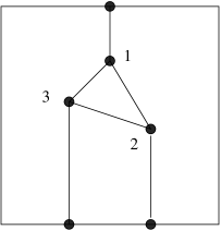
Figure 6: A network of three vertices with $\widehat{E}>0$.

consider the system corresponding to the general system (7.10).

$$\begin{array}[]{c}({\bf T}^{1}+{\bf e}_{2})\cdot{\bf e}_{2}=0,\;\;\;({\bf T}^{1}-{\bf T}^{2})\cdot{\bf q}^{12}=0,\;\;\;\;({\bf T}^{1}-{\bf T}^{3})\cdot{\bf q}^{13}=0,\\ ({\bf T}^{2}-{\bf T}^{3})\cdot{\bf q}^{23}=0,\;\;\;\;({\bf T}^{2}-{\bf e}_{2})\cdot{\bf e}_{2}=0,\;\;\;\;\;({\bf T}^{3}-{\bf e}_{2})\cdot{\bf e}_{2}=0.\\ \end{array}$$ (7.14)

We prove that the system (7.14) has no solutions. Indeed, the last two equations imply ${\bf T}^{2}=t_{2}{\bf e}_{1}+{\bf e}_{2}$, ${\bf T}^{3}=t_{3}{\bf e}_{1}+{\bf e}_{2}$, for some scalars $t_{2},t_{3}$. Next, the first equation in the second row of (7.14) yields $(t_{2}-t_{3}){\bf e}_{1}\cdot{\bf q}^{23}=0$, and thus $t_{2}=t_{3}=t$. Substituting ${\bf T}^{2}={\bf T}^{3}=t{\bf e}_{1}+{\bf e}_{2}$ into the second and third equations in the first row of (7.14) we obtain

$$\begin{array}[]{c}({\bf T}^{1}-t{\bf e}_{1}-{\bf e}_{2})\cdot{\bf q}^{12}=0,\\ ({\bf T}^{1}-t{\bf e}_{1}-{\bf e}_{2})\cdot{\bf q}^{13}=0.\\ \end{array}$$ (7.15)

Since ${\bf q}^{12},{\bf q}^{13}$ are non-collinear, (7.15) yields ${\bf T}^{1}=t{\bf e}_{1}+{\bf e}_{2}$, which contradicts the first equation in the first row of (7.14).
Example 3. Next, consider a rectangular network of four vertices in Fig. 7.

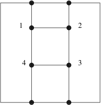
Figure 7: A network of four vertices with $\widehat{E}>0$.

The system (7.10) for this example becomes

$$\begin{array}[]{c}({\bf T}^{1}-{\bf T}^{2})\cdot{\bf e}_{1}=0,\;\;\;\;({\bf T}^{1}-{\bf T}^{4})\cdot{\bf e}_{2}=0,\;\;\;\;({\bf T}^{2}-{\bf T}^{3})\cdot{\bf e}_{2}=0,\;\;\;\;({\bf T}^{3}-{\bf T}^{4})\cdot{\bf e}_{1}=0,\\ ({\bf T}^{1}+{\bf e}_{2})\cdot{\bf e}_{2}=0,\;\;\;\;\;\;({\bf T}^{2}+{\bf e}_{2})\cdot{\bf e}_{2}=0,\;\;\;\;({\bf T}^{3}-{\bf e}_{2})\cdot{\bf e}_{2}=0,\;\;\;\;({\bf T}^{4}-{\bf e}_{2})\cdot{\bf e}_{2}=0.\\ \end{array}$$ (7.16)

The last two equations in the second row of (7.16) yield ${\bf T}^{3}=t_{3}{\bf e}_{1}+{\bf e}_{2}$, ${\bf T}^{4}=t_{4}{\bf e}_{1}+{\bf e}_{2}$, with some scalars $t_{3},t_{4}$. Next, the second and third equations in the first row of (7.16) produce ${\bf T}^{1}=t_{1}{\bf e}_{1}+{\bf e}_{2}$, ${\bf T}^{2}=t_{2}{\bf e}_{1}+{\bf e}_{2}$, which contradict, respectively, the first and second equations in the second row.

The three examples above seem to indicate that two basic building blocks for networks with $\widehat{E}>0$ (strong blow up) are triangles (Fig. 6) and rectangles aligned with the edges of $\Omega$ (Fig. 7). Misaligned rectangular structures such as shown in Fig. 8 would produce $\widehat{E}=0$ (weak blow up).

7.3 Quasi-triangulated graphs

7.3.1 Definition of quasi-triangulated graphs. Solvability of the system (5.34)

The network $\Gamma$ partitions $\Omega$ into a a disjoint union of convex polygons, which are called Delaunay cells. When points ${\bf x}^{j}$ are distributed randomly in $\Omega$, the interior Delaunay cells are typically triangles. This simple but important fact can be explained as follows. The edges of Voronoi tessellation are perpendicular bisectors of the edges of Delaunay cells. If an interior Delaunay cell is, for instance, a quadrilateral, then any two vertices lying on a diagonal cannot be neighbors, and therefore the point of intersection of four edges of the Voronoi tessellation must be equidistant from the four vertices. This means that a convex quadrilateral may be a Delaunay cell only if all four vertices lie on a circle. When the vertices of the network are randomly placed, the likelihood of four (or more) points lying on the same circle is small. It is natural to call such cells the defect cells. Therefore, most of the interior Delaunay cells of a random network are triangles. Other polygonal cells (quadrilateral, pentagonal etc.) are typically small in number, isolated and are likely to be unstable in the actual flow.

Since the exterior edges of the network are vertical, the cells adjacent to the boundary are typically quadrilateral. An example of a generic network is shown on Fig. 8.

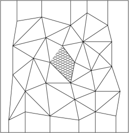
Figure 8: An example of the network. The shaded quadrilateral represents a defect cell.

Next, we define a broad class of graphs containing generic Delaunay-type networks. The graphs in this class are called quasi-triangulated, because of the presence of triangular cells. The number of triangular cells may be relatively small, as indicated by the examples below. We show that for quasi-triangulated graphs the leading term in the asymptotics can be effectively computed by minimizing the functional $\widehat{Q}$, that is the minimum is unique and can be found by solving the linear system (5.34). We also show that the crucial estimate (5.29) holds even for more general graphs which contain a ”spanning” quasi-triangulated subgraph.

Given an arbitrary network graph $\Gamma$, we define its maximal quasi-triangulated subgraph $\Gamma_{M}$ by the following iterative procedure.
Step 1. Consider interior vertices which are connected to $\partial\Omega^{-}$ and call these vertices generation one vertices. All interior edges connecting these vertices are generation one edges. Add all generation one edges and vertices to the subgraph.
Step 2. Consider all remaining vertices which are connected to the vertices of the subgraph by at least two non-collinear edges. These vertices and edges belong to generation two. Add them to the subgraph. Note that the non-collinearity condition leads to formation of ”supportive triangles”.
Step 3. Repeat step 2 until no more vertices can be added.

If the maximal quasi-triangulated subgraph $\Gamma_{M}$ contains all interior vertices of $\Gamma$, we call the graph $\Gamma$ quasi-triangulated. It turns out that for quasi-triangulated graphs the system (5.34) is ”almost uniquely” solvable, that is two solutions differ by a vector of the form $t{\bf w}_{0}$, where ${\bf w}_{0}$ is defined by (5.36), and the value of the form $Q$ for these solutions is the same.

Proposition 7.1

Suppose that the network graph $\Gamma$ is quasi-triangulated. Then there is a unique solution of the system (5.34), up to a horizontal translation.

This proposition is proved in Appendix B.

7.3.2 Examples of quasi-triangulated graphs

First we observe that a restriction to $\Omega$ of a periodic rectangular lattice is not quasi-triangulated. By contrast, a periodic triangular lattice restricted to $\Omega$ is quasi-triangulated. (see Fig. 9).

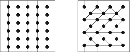
Figure 9: A rectangular graph on the left is not quasi-triangulated. Clearly, in this case $\Gamma_{F}=\Gamma^{-}$. The triangular graph on the right is quasi-triangulated.

In fact, if a network $\Gamma$ is not periodic, but all of its interior Delaunay cells are triangles, then $\Gamma$ is quasi-triangulated. The converse is false (see an example in Fig. 11). This means that the quasi-triangulation property is more general than triangulation property. In [4] we considered a class of graphs containing a triangulated path (see Fig. 10). In Fig 11, we present two examples showing that a quasi-triangulated graph need not contain a triangulated path. On the other hand, a graph containing a triangulated path is not necessarily quasi-triangulated. However, when a triangulated path exists, it must be contained in the maximal quasi-triangulated subgraph. Therefore, in this case the maximal quasi-triangulated subgraph is spanning (”extends from top to bottom”). Below in section 7.4.1 we show that this condition is sufficient for positivity of the minimum of $\widehat{Q}$.

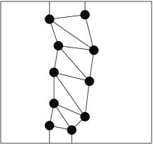
Figure 10: A triangulated path.

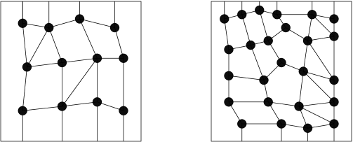
Figure 11: The graph on the left is quasi-triangulated but does not contain a triangulated path. The graph on the right contains a triangulated path, but is not quasi-triangulated.

7.4 Strong blow up of $\lambda^{\star}$. Percolating rigidity networks

7.4.1 Quasi-triangulated subgraphs

For the rest of this section, we consider the steady flow of the suspension corresponding to the boundary conditions (7.5) with the extension rate $\epsilon=1$.

We shall say that a network is a percolating rigidity graph when the crucial estimate (5.29) holds. In this subsection we show that quasi-triangulated graphs are percolating rigidity graphs. Moreover, a graph has percolating rigidity even when it is not quasi-triangulated but contains a spanning quasi-triangulated subgraph.

Proposition 7.2

Suppose that the boundary conditions are given by (7.5) and the network graph $\Gamma$ contains a spanning quasi-triangulated subgraph. Then $\Gamma$ is a percolating rigidity graph. Consequently, the extensional effective viscosity $\lambda^{\star}$ of suspensions corresponding to such networks is $O(\delta^{-3/2})$.

The proof of this proposition is given in Appendix C.

7.4.2 Networks containing a vertical path. Periodic square networks

We now present another class of percolating rigidity graphs. Namely, these are graphs that contain a path connecting $\partial\Omega^{+}$ and $\partial\Omega^{-}$, such that all edges in this path are oriented along ${\bf e}_{2}$-direction (vertical). The simplest representative of this class of graphs is a periodic square lattice. A periodic square graph does not contain a spanning quasi-triangulated subgraph (in this case $\Gamma_{M}$ is just a path which consists of the vertices adjacent to $\partial\Omega^{-}$, see Fig. 9). However, the estimate (5.29) holds for a periodic square graph such as the one shown on Fig. 9. This follows from the more general criterion

Proposition 7.3

Suppose that a network graph $\Gamma$ contains a path $\Gamma^{\pm}$ such that

i) it connects $\partial\Omega^{+}$ and $\partial\Omega^{-}$,

ii) all edges of $\Gamma^{\pm}$ are vertical.

Then $\Gamma$ is a percolating rigidity graph.

As noted above, if a path $\Gamma^{\pm}$ has percolating rigidity, then the ”larger” graph $\Gamma$ is also a percolating rigidity graph. Therefore, we only need to show that a path of vertical edges has percolating rigidity, that is, the quadratic form $\widehat{Q}$ corresponding to such path is positive-definite.

For simplicity, consider a path containing three vertices. The argument can be directly generalized to an arbitrary number of vertices. As before, (5.29) will hold if the corresponding system (7.10) has no solutions. The latter now has the form

$$\begin{array}[]{c}({\bf T}^{1}-{\bf e}_{2})\cdot{\bf e}_{2}=0,\\ ({\bf T}^{1}-{\bf T}^{2})\cdot{\bf e}_{2}=0,\\ ({\bf T}^{2}-{\bf T}^{3})\cdot{\bf e}_{2}=0,\\ ({\bf T}^{3}+{\bf e}_{2})\cdot{\bf e}_{2}=0,\\ \end{array}$$ (7.17)

Introduce new unknown vectors $\widehat{\bf T}^{i}={\bf t}^{i}+{\bf e}_{2}$ $i=1,2,3$. The last equation of (7.17) yields $\widehat{\bf T}^{3}=t_{3}{\bf e}_{1}$, where $t_{3}$ is a scalar. Then from the third equation we obtain $\widehat{\bf T}^{2}=t_{2}{\bf e}_{1}$, and then the second equation yields $\widehat{\bf T}^{1}=t_{1}{\bf e}_{1}$, which contradicts the first equation. The contradiction shows that the system (7.17) has no solutions. The argument can be easily modified to show that if at least one of the edges of a path is non-vertical, then this path does not have percolating rigidity.

Proposition 7.3 shows that for rectangular lattices oriented parallel to the edges of $\partial\Omega$, asymptotics of extensional effective viscosity is of order $\delta^{-3/2}$ which corresponds to strong blow up. Asymptotic formulas in [11] also predict strong blow up of the extensional viscosity for cubic lattices. Thus our results are consistent with the results in [11]. We refer to section 8 for a more detailed comparison.

7.5 Weak blow up

In this section we present an example of a particle array for which the leading term in the asymptotics of $\lambda^{\star}$ is zero. Roughly speaking, the array in question is a rectangular lattice rotated so that none of its interior edges are vertical. Let ${\bf k}$ denote a unit vector non-collinear to either ${\bf e}_{1}$ or ${\bf e}_{2}$. The interior edges of the rectangular network in Fig. 12 are either parallel or perpendicular to ${\bf k}$, while the prescribed boundary velocities are parallel to ${\bf e}_{2}$. This misalignment will lead to weak blow up. To show that the system (7.10) is solvable, we first consider a single path connecting $\partial\Omega^{+}$ and $\partial\Omega^{-}$. This path may be any of the three such paths in Fig. 12. The argument we use admits a straightforward generalization to a network with an arbitrary number of vertices.

Figure 12: A rotated rectangular lattice of 12 vertices.

The system (7.10) written for the path has the form

$$\begin{array}[]{c}({\bf T}^{1}-{\bf e}_{2})\cdot{\bf e}_{2}=0,\\ ({\bf T}^{1}-{\bf T}^{2})\cdot{\bf k}=0,\\ ({\bf T}^{2}-{\bf T}^{3})\cdot{\bf k}=0,\\ ({\bf T}^{3}-{\bf T}^{4})\cdot{\bf k}=0,\\ ({\bf T}^{4}+{\bf e}_{2})\cdot{\bf e}_{2}=0,\\ \end{array}$$ (7.18)

For technical reasons it is convenient to introduce new unknowns ${\bf u}_{1}={\bf T}^{1}-{\bf e}_{2}$, ${\bf u}_{12}={\bf T}^{1}-{\bf T}^{2}$, ${\bf u}_{23}={\bf T}^{2}-{\bf T}^{3}$, ${\bf u}_{34}={\bf T}^{3}-{\bf T}^{4}$. The relations between ${\bf u}_{ij}$ and ${\bf T}^{i}$ are

$${\bf T}^{1}={\bf u}_{1}+2{\bf e}_{2},$$

$${\bf T}^{2}={\bf u}_{1}+2{\bf e}_{2}-{\bf u}_{12},$$

$${\bf T}^{3}={\bf u}_{1}+2{\bf e}_{2}-{\bf u}_{12}-{\bf u}_{23},$$

$${\bf T}^{4}={\bf u}_{1}+2{\bf e}_{2}-{\bf u}_{12}-{\bf u}_{23}-{\bf u}_{34}.$$ (7.19)

From the first four equations of (7.18) we see that ${\bf u}_{1}=t_{1}{\bf e}_{1}$, and ${\bf u}_{i,i+1}=t_{i,i+1}{\bf k}^{\bot}$, $i=1,2,3$, where ${\bf k}^{\bot}$ denotes a unit vector orthogonal to ${\bf k}$, and $t_{1},t_{i,i+1}$ are scalars. The problems of solving (7.18) is now reduced to finding $t_{1},t_{i,i+1}$ such that the fifth equation of (7.18) is satisfied. The fifth equation shows that

$${\bf T}^{4}=t_{4}{\bf e}_{1}-{\bf e}_{2},$$ (7.20)

where $t_{4}$ is a scalar. Equating (7.20) and (7.19) we obtain the equation for $t_{1},t_{12},t_{23},t_{34}$ and $t_{4}$:

$$t_{4}{\bf e}_{1}=t_{1}{\bf e}_{1}+{\bf e}_{2}-(t_{12}+t_{23}+t_{34}){\bf k}^{\bot}.$$ (7.21)

This yields two scalar equations

$$0=1-(t_{12}+t_{23}+t_{34}){\bf k}^{\bot}\cdot{\bf e}_{2},$$ (7.22)

and

$$t_{1}-t_{4}=(t_{12}+t_{23}+t_{34}){\bf k}^{\bot}\cdot{\bf e}_{1}.$$ (7.23)

The system of two equations (7.22),(7.23) for five unknowns has infinitely many nontrivial solutions as long as ${\bf k}^{\bot}\cdot{\bf e}_{2}\neq 0$ , that is, the interior edges of the path are non-vertical.

At the next step of construction, we consider the full lattice on Fig. 6 containing 12 vertices. The interior edges of the graph are oriented either by the unit vector ${\bf k}$ as above (longitudinal edges), or by ${\bf k}^{\bot}$ (latitudinal edges). We view the graph as the union of three paths of longitudinal edges extending from $\partial\Omega^{-}$ to $\partial\Omega^{+}$, with latitudinal edges connecting these paths. To obtain the desired example, we choose the vectors ${\bf T}^{i}$ for one of the paths, as explained above. Then we prescribe the same vectors to the corresponding vertices of two remaining paths. Now, if two neighbors ${\bf x}^{i}$ , ${\bf x}^{j}$ belong to different paths, then ${\bf T}^{i}={\bf T}^{j}$, so the corresponding equation $({\bf T}^{i}-{\bf T}^{j})\cdot{\bf k}^{\bot}=0$ of the system (7.10) is satisfied. When the neighbors ${\bf x}^{i},{\bf x}^{j}$ belong to the same path, the corresponding equation $({\bf T}^{i}-{\bf T}^{j})\cdot{\bf k}=0$ is satisfied by the choice of ${\bf T}^{i},{\bf T}^{j}$. Therefore, the whole system (7.10) in this case has infinitely many nontrivial solutions. Each of these solutions makes $\widehat{Q}$, and thus the leading term in the asymptotics of $\lambda^{\star}$, zero.

8 Comparison with some results for periodic cubic arrays in dimension three

The main objective of network approximation is to define effective properties for non-periodic deterministic or random arrays. While techniques of periodic homogenization are well developed ([3], [12], [10] and references therein), non-periodic geometries are much less understood. In the end of this section, we compare our results applied in particular case of a periodic square array (in dimension two) with the results of [11] obtained for cubic arrays in dimension three.

The effective viscosity of an infinite periodic suspension obtained in [11] is the fourth order tensor ${\mbox{\boldmath$\mu$}}^{\star}$ (in this section we use the notation from from [11]). In an effective flow with the constant strain rate $\gamma$, the effective stress is

$$S_{ij}^{0}=2\mu^{\star}_{ijkl}\gamma_{kl}-P\delta_{ij},$$ (8.1)

where $P$ is an effective pressure. The authors of [11] obtained the following formula for the components of ${\mbox{\boldmath$\mu$}}^{\star}$:

$$\mu^{\star}_{ijkl}=\frac{1}{2}\mu(1+\beta)(\delta_{ik}\delta_{jl}+\delta_{il}\delta_{jk}-\frac{2}{3}\delta_{ij}\delta_{kl})+\mu(\alpha-\beta)(\delta_{ijkl}-\frac{1}{2}\delta_{ij}\delta_{kl}),$$ (8.2)

where $\delta_{ijkl}=1$ if all indices are equal, otherwise $\delta_{ijkl}=0$. $\mu$ is the fluid viscosity, and $\alpha,\beta$ are functions of the small parameter $\epsilon$, related to the inter-particle distance $\delta$ as follows:

$$\epsilon=\frac{\delta}{2a+\delta}\approx\frac{\delta}{2a},\;\;\;{\rm as}\;\delta\to 0.$$ (8.3)

When the effective flow is incompressible, $\gamma_{ii}=0$, so the formula (8.2) simplifies to

$$\mu^{\star}_{ijkl}=\frac{1}{2}\mu(1+\beta)(\delta_{ik}\delta_{jl}+\delta_{il}\delta_{jk})+\mu(\alpha-\beta)\delta_{ijkl}.$$ (8.4)

For simple cubic lattices, up to the terms of order $O(1)$ in $\epsilon$, ([11])

$$\alpha=\frac{3}{16}\pi\epsilon^{-1}+\frac{27}{80}\pi\ln\epsilon^{-1},$$ (8.5)

and

$$\beta=\frac{1}{4}\pi\ln\epsilon^{-1}.$$ (8.6)

Suppose that the imposed effective flow is a steady shear with the velocity ${\bf v}=(\kappa x_{3},0,0)$ (three-dimensional analogue of (A.1)), where $\kappa>0$ is a constant shear rate. The components of the corresponding strain rate tensor $\gamma$ are $\gamma_{13}=\gamma_{31}=\kappa>0$ and $\gamma_{ij}=0$ for other values of $(i,j)$. Then, using (8.4), we obtain from (8.1) that the only nonzero components of the effective deviatoric stress $2{\mbox{\boldmath$\mu$}}^{\star}{\mbox{\boldmath$\gamma$}}$ are

$$(2\mu^{\star}\gamma)_{13}=(2\mu^{\star}\gamma)_{31}=2\mu(1+\beta)\kappa.$$ (8.7)

Since $\alpha$ is not present in (8.7), the nonzero components of the deviatoric effective stress are of order $\ln\epsilon^{-1}$ and thus the shear effective viscosity calculated by the three-dimensional analogue of definition (3.5) is of order $\ln\epsilon^{-1}$ (weak blow up in dimension three). The weak blow up was not identified in [11], but it can be easily deduced from the formulas derived there.

In the case of an extensional flow, velocity vector ${\bf v}=(\kappa x_{1},\kappa x_{2},-2\kappa x_{3})$, (compare with (A.5)), where $\kappa>0$ is a constant extension rate. The strain rate tensor is

$${\mbox{\boldmath$\gamma$}}=\left(\begin{array}[]{ccc}\kappa&0&0\\ 0&\kappa&0\\ 0&0&-2\kappa\\ \end{array}\right)$$ (8.8)

Then, using (8.1) and (8.4) we obtain the deviatoric stress

$$2{\mbox{\boldmath$\mu$}}^{\star}{\mbox{\boldmath$\gamma$}}=\left(\begin{array}[]{ccc}L&0&0\\ 0&L&0\\ 0&0&-2L,\\ \end{array}\right)$$ (8.9)

where

$$L=2\kappa\mu(1+\beta)+\kappa\mu(\alpha-\beta).$$ (8.10)

Components of the deviatoric stress contain $\alpha$ and are therefore of order $\epsilon^{-1}$. Consequently, the extensional effective viscosity is of order $\epsilon^{-1}$ (strong blow up in dimension three).

Although Noonan and Keller did not address the issue of weak versus strong blow up for the effective viscosity in [11], the formulas (8.5)- (8.10) are consistent with the results for square lattices in Section 6 of this paper in the following sense. If a periodicity cell corresponding to a simple cubic lattice is subjected to a uniform shear (extensional) flow, then the straightforward calculation presented above shows that the shear (extensional) effective viscosity exhibits weak (strong) blow up. However, for other lattice types such as BCC and FCC, formulas from [11] imply strong blow up of both viscosities, while our approach leads to the weak blow up of the shear viscosity for all two-dimensional lattices. Perhaps, this can be attributed to the fact that in [11] effective viscosity is defined in a different way, as explained in the introduction. In particular, our definition takes into account boundary effects which are known to be essential in rheological measurements ([17], [15]). Considerations based on infinite periodic lattices cannot capture these boundary effects. Futhermore, if our approach is applied to a rectangular periodic lattice in a rectangular domain chosen so that lattice periodicity is preserved, then our results are consistent with [11].

9 Conclusions

We have studied properties of the network approximation of the shear effective viscosity $\mu^{\star}$ and extensional effective viscosity $\lambda^{\star}$ of two-dimensional flows of concentrated suspensions with complex geometry. The flow domain was chosen to be a square, upper and lower sides of which represented the physical flow boundary, while the other two sides were assumed to be free surfaces.

A small inter-particle distance parameter $\delta$ was used to describe the high concentration regime for particle arrays which are not necessarily periodic (i. g. random). In the recent paper [14] by Sierou and Brady, the high frequency dynamic viscosity of concentrated suspensions (see [17]) was calculated as a function of volume fraction $\phi$ by means of accelerated Stokesian dynamics simulations. Numerical results indicate a singular behaviour of the effective viscosity as $\phi$ approaches the maximal close packing fraction $\phi_{rcp}$. We quote here from ([14]): ”… The exact form of this singular behaviour is not known. Results from lubrication theory for cubic lattices would suggest that the singular form should consist both of $1/\epsilon$ and $\ln\epsilon$, where $\epsilon=1-(\phi/\phi_{rcp})^{1/3}$, but the relative amount of each term is unknown… As far as we are able to tell at this point, the $\ln\epsilon$ behaviour accurately describes the numerical data.”

When the volume fraction is (approximately) constant over the flow region, $\epsilon\approx\delta$. One of the objectives of our investigation was to address the issue of the unexpectedly weak blow up in [14], and determine the asymptotic order of the effective viscosity coefficients as $\delta\to 0$. Our analysis of the shear viscosity $\mu^{\star}$, based on the discrete network approximation, showed that $\mu^{\star}=O(\delta^{-1/2})$ as $\delta\to 0$, while the formal estimate based of the local lubrication analysis would give a higher rate $O(\delta^{-3/2})$. In dimension three, the corresponding rates, given by the network approximation, are, respectively, $\ln\delta$ and $\delta^{-1}$ (see [4]). Our analysis offers an explanation of the weak blow up of the shear viscosity. This analysis is also consistent with the numerical simulations in [14] up to the difference in the space dimension.

We also show that the asymptotic order of the extensional viscosity $\lambda^{\star}$ depends on the geometry of the particle array. For generic disordered arrays the network partitions the domain into polygons (Delaunay cells), most of which are triangles. We have showed that for these generic arrays $\lambda^{\star}=O(\delta^{-3/2})$. The same asymptotic rate is obtained for a larger class of networks called quasi-triangulated. In a quasi-triangulated network, the percentage of triangular cells may be relatively small, but the subnetwork containing triangular cells must be spanning. Another class of networks for which $\lambda^{\star}=O(\delta^{-3/2})$ consists of rectangular periodic arrays aligned with the boundary of the flow. More generally, the same rate is obtained for arrays containing a single spanning chain of neighboring particles, perpendicular to the part of the boundary where the velocity is prescribed.

We show that in case of the strong blow up, the leading term in the asymptotics of $\lambda^{\star}$ can be uniquely determined by solving a simplified linear system of the network equations, provided the array is quasi-triangulated. The simplified system, obtained by neglecting rotational and pairwise shear motions of particles, provides an efficient computational tool for evaluating the dependence of the effective viscosity on the geometry of the particle array and external boundary conditions. When a network contains neither a spanning triangulated subgraph, nor a spanning vertical path, the extensional effective viscosity can be of order $\delta^{-1/2}$. This weak blow up is obtained, for instance, in the case of a periodic rectangular lattice, with interior edges misaligned with the orientation of the prescribed boundary data.

Our results imply that the ratio of $\lambda^{\star}$ to $\mu^{\star}$ for generic disordered particle arrays is $O(\delta^{-1})$. By contrast, in a Newtonian fluid this ratio depends only on the space dimension. Therefore, our results indicate possible non-Newtonian behaviour of the effective fluid.

10 Acknowledgments

The authors wish to thank Professor John F. Brady for bringing the work [14] to their attention. Work of Leonid Berlyand was supported in part by NSF grant DMS-0204637. Work of Alexander Panchenko was supported in part by the ONR grant N00014-001-0853.

Appendix A Shear and extensional flows. Ratio of the viscosities in a Newtonian fluid

The following types of flows are relevant to our investigation.

Shear flow. Consider the steady shear flow a homogeneous fluid characterized by the constant shear rate $\gamma$. The velocity is given by

$${\bf v}^{0}_{sh}=\left(\begin{array}[]{c}\gamma x_{2}\\ 0\end{array}\right).$$ (A.1)

and the strain rate tensor is

$${\mbox{\boldmath$e$}}_{sh}^{0}=\frac{1}{2}\left(\begin{array}[]{cc}0&\gamma\\ \gamma&0\end{array}\right).$$ (A.2)

Since the stress tensor is symmetric and independent of ${\bf x}$,

$$E^{0}=\int_{\Omega}\mbox{\boldmath$S$}^{0}\cdot{\mbox{\boldmath$e$}}_{\it sh}^{0}d{{\bf x}}=\frac{1}{2}S^{0}_{12}\gamma|\Omega|,$$ (A.3)

where $|\Omega|=\int_{\Omega}d{\bf x}$.

In the case of a homogeneous Newtonian fluid with viscosity $\mu$, $\mbox{\boldmath$S$}^{0}=2\mu{\mbox{\boldmath$e$}}_{sh}^{0}-PI$, so that $S^{0}_{12}=\mu\gamma$. Using the formula (3.4) we obtain

$$\mu^{\star}=\mu,$$ (A.4)

as expected.

Extensional flow. In this case the fluid is being extended in the horizontal direction and simultaneously contracted in the vertical direction at the same constant rate $\varepsilon$. The velocity is

$${\bf v}^{0}_{\it ext}=\left(\begin{array}[]{c}\varepsilon x_{1}\\ -\varepsilon x_{2}\end{array}\right),$$ (A.5)

and

$${\mbox{\boldmath$e$}}_{ext}^{0}=\left(\begin{array}[]{cc}\varepsilon&0\\ 0&-\varepsilon\end{array}\right).$$ (A.6)

For a homogeneous Newtonian fluid, $\mbox{\boldmath$S$}^{0}_{ext}=2\mu{\mbox{\boldmath$e$}}^{0}_{ext}-PI$, and thus $S^{0}_{11}=2\mu\varepsilon-P$, $S^{0}_{22}=-2\mu\varepsilon-P$. Next using the definition (3.7) we obtain

$$\lambda^{\star}=4\mu.$$ (A.7)

Therefore, for a Newtonian effective fluid the ratio $\lambda^{\star}/\mu^{\star}$ equals $4$ (in two dimensions).

Appendix B Proof of Proposition 7.1

The proposition 7.1 will be proved if we prove the following

Proposition B.1

Suppose the network graph $\Gamma$ is quasi-triangulated. Then every solution of the homogeneous system (5.37) is of the form $t{\bf w}_{0}$ where $t$ is arbitrary real and ${\bf w}_{0}$ is given by (5.36).

Proof. First note that (5.37) is Euler-Lagrange system for the functional

$$Q_{hom}=\frac{1}{2}A{\bf z}\cdot{\bf z}=\displaystyle{\frac{1}{2}\sum_{i=1}^{N}\sum_{j\in{\cal N}_{i}}C^{ij}_{sp}(({\bf T}^{i}-{\bf T}^{j})\cdot{\bf q}^{ij})^{2}+\sum_{i\in I}C_{1}^{i}({\bf T}^{i}\cdot{\bf q}^{i})^{2}.}$$ (B.1)

Clearly the minimum of $Q_{hom}$ is zero. Thus every solution of (5.37) is a minimizer of $Q_{hom}$. On the other hand, $Q_{hom}({\bf T}^{1},\ldots{\bf T}^{N})=0$ if and only if the vectors ${\bf T}^{i}$ satisfy the system of equations

$$\begin{array}[]{cc}({\bf T}^{i}-{\bf T}^{j})\cdot{\bf q}^{ij}=0,&~{}~{}~{}~{}i=1,2\ldots N,~{}~{}j\in{\cal N}_{i}\\ {\bf T}^{i}\cdot{\bf q}^{i}=0,&i\in I.\end{array}$$ (B.2)

Therefore, a vector ${\bf z}=({\bf T}^{1},\ldots{\bf T}^{N})^{T}$ solves (5.37) if and only if ${\bf T}^{i},i=1,\ldots,N$ solve (B.2). The solvability of (B.2) will be directly linked to the geometric structure of the graph $\Gamma$. We begin by observing that ${\bf q}^{i}=\pm{\bf e}_{2}$. Thus the second set of equations in (B.2) yields

$${\bf T}^{i}=t^{i}{\bf e}_{1},i\in I,$$ (B.3)

that is, ${\bf T}^{i}$ are horizontal for all boundary vertices. Next, consider boundary vertices ${\bf x}^{i},i\in I^{-}$ (these are vertices connected to $\partial\Omega^{-}$), and recall that they belong to a path $\Gamma^{-}$, edges of which are interior edges of $\Gamma$. Hence, if $i_{1}\in I^{-}$, then there is at least one $i_{2}\in I^{-},i_{2}\neq i_{1}$ such that ${{\bf x}}^{i_{1}}$ and ${{\bf x}}^{i_{2}}$ are connected by an interior edge $b^{i_{1}i_{2}}$. Using the first set of equations in (B.2) and (B.3) we obtain

$$({\bf T}^{i_{1}}-{\bf T}^{i_{2}})\cdot{\bf q}^{i_{1}i_{2}}=(t^{i_{1}}-t^{i_{2}}){\bf e}_{1}\cdot{\bf q}^{i_{1}i_{2}}=0.$$ (B.4)

Furthermore, $b^{i_{1}i_{2}}$ is non-vertical, that is, ${\bf q}^{i_{1}i_{2}}\cdot{\bf e}_{1}\neq 0$, which yields $t^{i_{1}}=t^{i_{2}}$. Since each ${\bf x}^{i},i\in I^{-}$ is connected to at least one other, we obtain

$${\bf T}^{i}=t{\bf e}_{1},~{}~{}~{}~{}i\in I^{-},$$ (B.5)

with the same scalar $t$.

Since the graph is quasi-triangulated, there exists an interior vertex ${{\bf x}}^{l_{1}}\in\Gamma$ , ${{\bf x}}^{l_{1}}\notin\Gamma^{-}$, connected to at least two vertices ${{\bf x}}^{i_{1}},{{\bf x}}^{i_{2}},i_{1},i_{2}\in I^{-}$ by non-collinear edges. Then, using the first set of equations in (B.2) we obtain

$$\begin{array}[]{c}({\bf T}^{l_{1}}-t{\bf e}_{1})\cdot{\bf q}^{l_{1},i_{1}}=0,\\ ({\bf T}^{l_{1}}-t{\bf e}_{1})\cdot{\bf q}^{l_{1},i_{2}}=0.\end{array}$$ (B.6)

Since ${\bf q}^{l_{1},i_{1}}$ and ${\bf q}^{l_{1},i_{2}}$ are linearly independent, (B.6) yields ${\bf T}^{l_{1}}=t{\bf e}_{1}$. Next, let $G_{1}$ be the union of $\Gamma^{-}$, ${{\bf x}}^{l_{1}}$ and all the edges which connect ${{\bf x}}^{l_{1}}$ to $\Gamma^{-}$. Using the definition of the quasi-triangulated graph again, we find a vertex ${{\bf x}}^{l_{2}}$, not contained in $G_{1}$, and connected to $G_{1}$ by two non-collinear edges. Repeating the argument following (B.6), we see that ${\bf T}^{l_{2}}=t{\bf e}_{1}$. Then we choose $G_{2}$ to be the union of $G_{1}$, ${{\bf x}}^{l_{2}}$ and all edges of $\Gamma$ which connect them. Repeating the process we find the vertex ${{\bf x}}_{l_{3}}$ and continue until we obtain

$${\bf T}^{i}=t{\bf e}_{1},~{}~{}~{}~{}~{}~{}~{}i=1,\dots N$$ (B.7)

with the same scalar $t$. This means that every solution of (B.2) is of the form $t{\bf w}_{0}$. Since solution spaces of (B.2) and (5.37) are the same, the proposition is proved.

The following discrete Korn inequality follows immediately from the Proposition B.1.

Corollary B.1

Suppose that $\Gamma$ is quasi-triangulated. Let $W\subset{\bf R}^{2N}$ be the one-dimensional subspace spanned by ${\bf w}_{0}$ from (5.36), and let $W^{\bot}$ denote the orthogonal complement of $W$ in ${\bf R}^{2N}$. Also, let $Q_{hom}$ and $A$ be, respectively the quadratic form defined in (B.1) and its matrix. Then there is a constant $C>0$ such that the Korn-type inequality

$$\frac{1}{2}A{\bf z}\cdot{\bf z}=Q_{hom}({\bf z})\geq C{\bf z}\cdot{\bf z}$$ (B.8)

holds for all ${\bf z}\in W^{\bot}$.

Another straightforward corollary is as follows.

Corollary B.2

Suppose that $\Gamma$ is quasi-triangulated. Then the system

$$A{\bf z}={\bf f}$$

has a unique solution ${\bf z}\in W^{\bot}$ provided ${\bf f}\bot W$.

Remark. The projection $P_{W}$ onto the subspace $W$ is defined by

$$P_{W}{\bf z}=\frac{{\bf z}\cdot{\bf w}_{0}}{N}{\bf w}_{0}.$$

In terms of vectors ${\bf T}^{i}$,

$$P_{W}({\bf T}^{1},{\bf T}^{2},\ldots{\bf T}^{N})=\frac{\sum_{i=1}^{n}T^{i}_{1}}{N}{\bf w}_{0}$$

Therefore, using the definition of ${\bf f}$ in terms of ${\bf R}^{i}$, we can write the condition ${\bf f}\bot W$ as

$$\sum_{i=1}^{n}R^{i}_{1}=\sum_{i=1}^{N}{\bf R}^{i}\cdot{\bf e}_{1}=0$$ (B.9)

The vectors ${\bf R}^{i}$ in (5.32) satisfy (B.9), so that ${\bf f}$ in (5.35) with $R^{i}$ defined by (5.32) is orthogonal to $W$. This gives the unique solvability of the network equations (5.34).

Corollary B.3

Suppose that $\Gamma$ is quasi-triangulated. Then there is a unique ${\bf z}^{*}\in W^{\bot}$ such that every solution of (5.34) is of the form ${\bf z}^{*}+t{\bf w}_{0}$, where $t{\bf w}_{0}\in W$.

This means that solution of the network equations (5.34) is unique up to a horizontal translation.

Appendix C Proof of proposition 7.2

Proof. First we observe that the form $\widehat{Q}$ is a sum of non-negative terms, each of which corresponds to an edge of the network graph $\Gamma$. Removal of an edge from $\Gamma$ corresponds to deletion of one non-negative term in $\widehat{Q}$. This means that for each subgraph $\Gamma^{\prime}$ of $\Gamma$, $\widehat{Q}(\Gamma)\geq\widehat{Q}(\Gamma^{\prime})$. Next we choose $\Gamma^{\prime}$ to be the maximal quasi-triangulated subgraph of $\Gamma$. We show that $\min\widehat{Q}(\Gamma^{\prime})>0$. Indeed, $\min\widehat{Q}(\Gamma^{\prime})=0$ if and only if the corresponding system (7.10) has a solution. To show that this system has no solutions, introduce new unknowns $\hat{\bf T}^{i}={\bf T}^{i}-{\bf e}_{2}$. Then from (7.10) we obtain

$$(\hat{\bf T}^{i}-\hat{\bf T}^{j})\cdot{\bf q}^{ij}=0,$$ (C.1)

$$\hat{\bf T}^{i}\cdot{\bf q}^{i}=\begin{cases}-2\;\;\;\;{\rm when}\;i\in I^{+}&\\ 0\;\;\;\;{\rm when}\;i\in I^{-}.&\\ \end{cases}$$ (C.2)

Since the vectors ${\bf q}^{i}$ are vertical, (C.2) yields

$$\hat{\bf T}^{i}=t^{i}{\bf e}_{1},\;\;\;\;i\in I^{-},$$ (C.3)

where $t^{i}$ is a constant. Recall that $\Gamma$ contains a path $\Gamma^{-}$ which consists of all boundary vertices connected to $\partial\Omega^{-}$ and all interior edges connecting these vertices. Hence, each ${\bf x}^{i_{1}},i_{1}\in I^{-}$ has a neighbor ${\bf x}^{i_{2}},i_{2}\in I^{-}$ and thus $(t^{i_{1}}-t^{i_{2}}){\bf e}_{1}\cdot{\bf q}^{i_{1}i_{2}}=0$ from (C.1). Since two boundary vertices cannot be joined by a vertical edge, ${\bf e}_{1}\cdot{\bf q}^{i_{1}i_{2}}\neq 0$. This implies that all $t^{i},i\in I^{-}$ are equal, that is

$$\hat{\bf T}^{i}=t{\bf e}_{1},i\in I^{-},$$ (C.4)

where $t$ is a constant. Next, consider the boundary path $\Gamma^{-}$. By definition of $\Gamma^{\prime}$ there is a vertex ${\bf x}^{j_{1}},j_{1}\not\in I^{-}$ connected to the boundary vertices ${\bf x}^{i_{1}},{\bf x}^{i_{2}}$, $i_{1},i_{2}\in I^{-}$ by non-collinear edges of $\Gamma$. Then from (C.1) and (C.4) we have

$$\begin{array}[]{c}(\hat{\bf T}^{j_{1}}-t{\bf e}_{1})\cdot{\bf q}^{j_{1},i_{1}}=0,\\ (\hat{\bf T}^{j_{1}}-t{\bf e}_{1})\cdot{\bf q}^{j_{1},i_{2}}=0.\\ \end{array}$$

Since ${\bf q}^{j_{1},i_{1}}$ and ${\bf q}^{j_{1},i_{2}}$ are linearly independent, we obtain $\hat{\bf T}^{j_{1}}=t{\bf e}_{1}$. Now this argument can be used recursively. Next we choose $G_{1}$ to be the union of vertices ${\bf x}^{i},i\in I^{-},{\bf x}^{j_{1}}$ and the edges of $\Gamma^{\prime}$ which connect these vertices. Repeating the argument, we find a vertex ${\bf x}^{j_{2}}\not\in G_{1}$, connected to at least two vertices of $G_{1}$ by non-collinear edges, which yields $\hat{\bf T}^{j_{2}}=t{\bf e}_{1}$, and so on, until we obtain $\hat{\bf T}^{i}=t{\bf e}_{1}$ for all vertices ${\bf x}^{i}$ which belong to $\Gamma^{\prime}$. By assumption, $\Gamma^{\prime}$ contains at least one vertex ${\bf x}^{+}\in I^{+}$. But then $\hat{\bf T}^{+}\cdot{\bf q}^{+}=-t{\bf e}_{1}\cdot{\bf e}_{2}=0$ which contradicts (C.2). This contradiction shows that the system (C.1), (C.2) has no solutions.

References

- [1] Batchelor, G. K. & Green, J. T. 1972 The determination of the bulk stress in a suspension of spherical particles to order . J. Fluid Mech. 56 Part 3,401–427.
- [2] Bakhvalov, N. & Panasenko, G. 1989 Homogenization: averaging processes in periodic media. Kluwer.
- [3] Bensoussan, A., Lions, J. L., & Papanicolaou, G. 1978 Asymptotic analysis in periodic structures. North-Holland.
- [4] Berlyand, L., Borcea, L & Panchenko, A. 2003 Network approximation for effective viscosity of concentrated suspensions with complex geometries. SIAM Journ. Math. Anal., to appear.
- [5] Berlyand, L. & Kolpakov, A. 2001 Network approximation in the limit of small inter-particle distance of the effective properties of a high-contrast random dispersed composite. Arch. Rat. Mech. Anal. 159, 179–227.
- [6] Carreau, P. J. & Cotton, F. 2002 Rheological properties of concentrated suspensions. In: Transport processes in bubbles, drops and particles. D. De Kee and R. P. Chhabra, eds., Taylor & Fransis.
- [7] Coussot, P. 2002 Flows of concentrated granular mixtures. In: Transport processes in bubbles, drops and particles. D. De Kee adn R. P. Chhabra, eds., Taylor & Fransis.
- [8] Einstein, A. 1906 Eine neue Bestimmung der Moleküldimensionen, Annln. Phys. 19 p. 289 and 34 p. 591.
- [9] Frankel, N. A. & Akrivos, A. 1967 On the Viscosity of a Concentrated Suspension of Solid Spheres. Chemical Engineering Science 22, 847–853.
- [10] Jikov, V., Kozlov, S. & Oleinik, O. 1994 Homogenization of differential operators and integral functionals. Springer.
- [11] Nunan. K. C. & Keller, J. B. 1984 Effective viscosity of periodic suspensions Journ. Fluid Mech. 142, 269–287.
- [12] Sanchez-Palencia, E. 1980 Non-homogeneous media and vibration theory. Springer.
- [13] Schowalter, W. R. 1978 Mechanics of Non-Newtonian Fluids. Pergamon Press.
- [14] Sierou, A. & Brady, J. F. 2001 Accelerated Stokesian Dynamic simulations. J. Fluid Mech. 448, 115–146.
- [15] Shikata, T & Pearson, D. S. 1994 Viscoelastic behavior of concentrated spherical suspensions. Journ. Rheology 38, 601–616.
- [16] Shook, C. A. & Rocko, M. C. 1991 Slurry flow. Principles and practice. Butterworth-Heinemann.
- [17] Van der Werff, J. C., de Kruif, C. G., Blom, C, & Mellema, J. 1989 Linear viscoelastic behavior of dense hard-sphere dispersions. Phys. Rev. A. 39, 795–807.