Variational bounds on the energy dissipation rate in body-forced shear flow

Abstract

A new variational problem for upper bounds on the rate of energy dissipation in body-forced shear flows is formulated by including a balance parameter in the derivation from the Navier-Stokes equations. The resulting min-max problem is investigated computationally, producing new estimates that quantitatively improve previously obtained rigorous bounds. The results are compared with data from direct numerical simulations.

1 Introduction

One of the outstanding open challenges for theoretical fluid mechanics in the $21^{\mathrm{st}}$ century is to derive rigorous results for turbulence directly from the fundamental equations of motion, the Navier-Stokes equations, without imposing ad hoc assumptions or uncontrolled closures. Exact results are extremely rare, but it is possible to derive rigorous and physically meaningful limits on some of the fundamental physical variables quantifying turbulent dynamics and transport. The bulk rate of energy dissipation is one such quantity of particular interest due to its production as a result of the turbulent cascade in the high Reynolds number vanishing viscosity limit. The derivation of mathematically rigorous bounds on the energy dissipation rate, and hence also a variety important quantities such as turbulent drag coefficients and heat and mass transport rates, has been a lively area of research in recent decades.

Beginning in the early 1960s, L.N. Howard and F.H. Busse pioneered the application of variational approaches for the derivation of rigorous—and physically relevant—bounds on the dissipation rate for boundary-driven flows; see their reviews [20, 1]. In the 1990s, P. Constantin and the senior author of this paper introduced the the so-called background flow method [6, 7] based on an old idea by Hopf [19]. The background method was soon improved by Nicodemus et al[22] who introduced an additional variational ‘balance’ parameter, and by the late 1990s Kerswell [21] had shown that the background method equipped with the balance parameter is dual to the Howard-Busse variational approach. Those theoretical techniques have been applied to many flows driven by boundary conditions, including shear flows and a variety of thermal convection problems [3, 4, 12, 5, 11, 26, 25].

Attention has recently turned as well to the derivation of quantitative variational bounds on the energy dissipation rate for body-forced flows. In these systems, the bulk (space and time averaged) dissipation rate per unit mass $\epsilon$ is proportional to the power required to maintain a statistically steady turbulent state. While body forces may be difficult to realize in experiments, they are easily implemented computationally and are the standard method of driving for direct numerical simulations (DNS) of turbulent flows.

Childress et al[2] applied a background-type method to body-forced flows in a periodic domain, focusing on dissipation estimates in terms of the magnitude of the applied force. In dimensionless variables they bounded $\epsilon$ in units of $(F^{3}\ell)^{1/2}$, where $F$ is the amplitude of the applied force per unit mass and $\ell$ is the (lowest) length scale in the force. The estimates were given in terms of the natural dimensionless control parameter, the Grashof number, $Gr:=F\ell^{3}/\nu^{2}$, where $\nu$ is the kinematic viscosity. In practice, $\epsilon$ is often measured in inviscid units of $U^{3}/\ell$ as a function of the Reynolds number $Re=U\ell/\nu$, where $U$ is a relevant velocity scale—an emergent quantity when the force is specified a priori. In both cases the dissipation is bounded on one side by that of the associated Stokes flow [17]. When bounds are expressed in terms of $Gr$, the Stokes limit is an upper bound, whereas when the estimates are in terms of $Re$ it is the lower limit.

Foias [13] was the first to derive an upper bound on

$$\beta:=\frac{\epsilon\ell}{U^{3}}\$$

in terms $Re$, but with an inappropriate prefactor dependence on the aspect ratio $\alpha=L/\ell$, where $L$ is the system volume, generally an independent variable from $\ell$ (see also [15, 16]). That analysis was recently refined by Foias and one of the authors of this paper [9] to an upper estimate of the form

$$\beta\leq c_{1}+\frac{c_{2}}{Re}\ ,$$

where the coefficients $c_{1}$ and $c_{2}$ are independent of $F,\ell,\nu$ and $\alpha$, depending only on the “shape” of the (square integrable) body force. (This in consistent with much of the conventional wisdom about the cascade in homogeneous isotropic turbulence theory [18, 10, 14] as well as with wind tunnel measurements [27] and DNS data [28].) Most recently, that approach was developed further by deriving a mini-max variational problem on the time averaged dissipation rate for a particular domain geometry [8]. Moreover, the variational problem was solved exactly at high Reynolds numbers to produce estimates on the asymptotic behavior of the energy dissipation as a function of $Re$ including the optimal prefactor.

In this paper we extend the results in [8] by introducing a balance parameter $c$, the analog of the variational parameter introduced by Nicodemus et al[22, 23, 24] for the background method. This parameter controls a balance between the quantity being bounded, the manifestly positive definite energy dissipation rate proportional to the $L^{2}$ norm of the rate of strain tensor, and the indefinite quantity derived from the power balance that is ultimately being extremized. Specifically we consider the flow of a viscous incompressible fluid bounded by two parallel planes with free-slip boundary conditions at the walls and periodic boundary conditions in the other two directions. The flow is maintained by a time-independent body force in the direction parallel to the walls. First we derive the Euler-Lagrange equations in the case $c=0$ (where the variational principle coincides with the one in [8]) and solve them numerically at finite $Re$. The full ($c>0$) Euler-Lagrange equations are quite complicated but they can also be solved numerically by using Newton method with the $c=0$ solution as an initial guess.

The rest of this paper is organized as follows. In Section 2 we introduce the problem and its variational formulation following [8]. In Section 3 we present the augmented variational problem and derive the variational equations, explaining how we go about solving them. In Section 4 we collect our numerical results, and in Section 5 we summarize the results discussing the challenges of this approach and future directions for research.

2 Statement of the problem

2.1 Notation

Consider a viscous incompressible Newtonian fluid moving between two parallel planes located at $y=0$ and $y=\ell$. Denote $x$ the stream-wise direction and $z$ be the span-wise direction. The velocity vector field satisfies free-slip boundary conditions at the two planes bounding the flow. We impose periodic boundary conditions in the other two directions. The motion of the fluid is induced by a steady body force ${\mathbf{f}}$ along the $x$ axis varying only in the $y$ direction.

The motion of the fluid is governed by Navier-Stokes equation

$$\frac{\partial{\mathbf{u}}}{\partial t}+({\mathbf{u}}\cdot\nabla){\mathbf{u}}+\nabla p=\frac{1}{Re}\Delta{\mathbf{u}}+{\mathbf{f}}$$ (1)

and the incompressibility condition,

$$\nabla\cdot{\mathbf{u}}=0\ .$$ (2)

Here $p({\mathbf{x}},t)$ is the pressure field, and $Re:=\frac{U_{\mathrm{rms}}\ell}{\nu}$ is the Reynolds number, where $U_{\mathrm{rms}}$ is the root-mean square velocity of the fluid. The problem is non-dimensionalized by choosing the unit of length to be $\ell$ and the unit for time to be $\ell/U_{\mathrm{rms}}$. Let $\langle\cdot\rangle$ stand for the space-time average. With this choice of units the velocity of the fluid ${\mathbf{u}}({\mathbf{x}},t)=(u,v,w)$ is space-time $L^{2}$-normalized to $1$:

$$\langle|{\mathbf{u}}|^{2}\rangle=\langle u^{2}+v^{2}+w^{2}\rangle=1\ .$$ (3)

Given $\epsilon$, is the space-time average energy dissipation rate in physical units, the non-dimensional energy dissipation rate $\beta$ is defined

$$\beta:=\frac{\ell\epsilon}{U_{\mathrm{rms}}^{3}}\ .$$ (4)

The body force ${\mathbf{f}}$ in (1) has the form

$${\mathbf{f}}({\mathbf{x}})=F\phi(y)\,{\mathbf{e}}_{x}\ ,$$

where the dimensionless shape function $\phi:[0,1]\to{\mathbb{R}}$ has zero mean and satisfies homogeneous Neumann boundary conditions, and is $L^{2}$-normalized:

$$\int_{0}^{1}\phi(y)\,{\mathrm{d}}y=0\ ,\quad\phi^{\prime}(0)=0=\phi^{\prime}(1)\ ,\quad\int_{0}^{1}\phi(y)^{2}\,{\mathrm{d}}y=1\ .$$

Now let $\Phi\in H^{1}([0,1])$ (where $H^{p}([0,1])$ is the space of functions defined on $[0,1]$ with $L^{2}$-integrable $p^{th}$ derivatives) be the potential defined by

$$\Phi^{\prime}=-\phi\ ,\quad\Phi(0)=0=\Phi(1)\ .$$

(Note that we are free to impose homogeneous Dirichlet conditions on $\Phi$ at both boundaries due to the zero mean condition on $\phi$.)

The spatial domain is $(x,y,z)\in[0,L_{x}]\times[0,1]\times[0,L_{z}]$ where $L_{x}$ and $L_{z}$ are the (non-dimensionalized) lengths in $x$ and $z$ directions. Free-slip boundary conditions at the walls are realized by

$$v=0\ ,\quad\frac{\partial u}{\partial y}=0=\frac{\partial w}{\partial y}\quad\mbox{ at }y=0\ ,1\ .$$ (5)

2.2 Variational problem for the energy dissipation rate

Here we follow [8] to derive the variational problem for upper bounds on the energy dissipation. Multiplying Navier-Stokes equation (1) by ${\mathbf{u}}$, integrate over the spatial domain, and average over time to obtain the energy dissipation rate

$$\beta:=\frac{1}{Re}\langle|\nabla{\mathbf{u}}|^{2}\rangle=\langle{\mathbf{f}}\cdot{\mathbf{u}}\rangle=F\langle\phi u\rangle=-F\langle\Phi^{\prime}u\rangle\ .$$ (6)

To remove the explicit appearance of the amplitude $F$ of the body force, multiply (1) by a vector field of the form $\psi(y){\mathbf{e}}_{x}$, where the multiplier function $\psi\in H^{2}([0,1])$ satisfies homogeneous Neumann boundary conditions $\psi^{\prime}(0)=0=\psi^{\prime}(1)$, and is not orthogonal to the shape function $\phi$. That is, $\langle\phi\psi\rangle\neq 0$. We will also use the derivative of $\psi$

$$\Psi\equiv\psi^{\prime}\in H^{1}([0,1])$$

which satisfies homogeneous Dirichlet boundary conditions $\Psi(0)=0=\Psi(1)$ and is not orthogonal to the shape potential $\Phi$, i.e., $\langle\Phi\Psi\rangle=\langle\phi\psi\rangle\neq 0$. We will call $\Psi$ a test function. Take the scalar product of (1) with $\psi(y){\mathbf{e}}_{x}$, integrate over the volume (integrating by parts by utilizing the boundary conditions) and take the long-time average to see that

$$-\langle\Psi uv\rangle=\frac{1}{Re}\langle\Psi^{\prime}u\rangle+F\langle\Phi\Psi\rangle\ .$$ (7)

Express the amplitude $F$ of the body force from (7) and insert into the expression for the energy dissipation (6) to obtain

$$\beta=\frac{\langle\Phi^{\prime}u\rangle\,\langle\Psi uv+\frac{1}{Re}\Psi^{\prime}u\rangle}{\langle\Phi\Psi\rangle}\ .$$ (8)

2.3 Mini-max upper bounds for $\beta$

A variational bound on $\beta$ may be obtained by first maximizing the right-hand side of (8) over all unit-normalized divergence-free vector fields ${\mathbf{u}}$ that satisfy the boundary conditions (5), and then minimizing over all choices of test functions $\Psi\in H^{1}([0,1])$ satisfying homogeneous Dirichlet boundary conditions. Then any solution of Navier-Stokes equation will have energy dissipation rate $\beta$ bounded from above by

$$\beta_{b}(Re)\equiv\min_{\Psi}\max_{{\mathbf{u}}}\frac{\langle\Phi^{\prime}u\rangle\,\langle\Psi uv+\frac{1}{Re}\Psi^{\prime}u\rangle}{\langle\Phi\Psi\rangle}\ .$$ (9)

In order to study the bound (9) above, the authors of [8] first evaluated (exactly)

$$\beta_{b}(\infty):=\min_{\Psi}\max_{{\mathbf{u}}}\frac{\langle\Phi^{\prime}u\rangle\,\langle\Psi uv\rangle}{\langle\Phi\Psi\rangle}\ ,$$

and then used this result to analyze the behavior of $\beta_{b}(Re)$ for finite $Re$. Since we are going to generalize that approach, we briefly recall the analysis:

The evaluation began with the proof that

$$\max_{{\mathbf{u}}}\,\langle\Phi^{\prime}u\rangle\langle\Psi uv\rangle=\frac{1}{\sqrt{27}}\,\sup_{y\in[0,1]}|\Psi(y)|\ .$$ (10)

This was accomplished by showing that the right-hand side of (10) is an upper bound for $\langle\Phi^{\prime}u\rangle\langle\Psi uv\rangle$ for any ${\mathbf{u}}$ in the class of vector field considered, and then explicitly constructing a sequence of unit-normalized divergence-free vector fields ${\mathbf{u}}^{(k)}=(u^{(k)},v^{(k)},w^{(k)})$ satisfying the boundary conditions (5) such that ${\mathbf{u}}^{(k)}$ saturate this bound in the limit $k\to\infty$, i.e.,

$$\lim_{k\to\infty}\langle\Phi^{\prime}u^{(k)}\rangle\langle\Psi u^{(k)}v^{(k)}\rangle=\frac{1}{\sqrt{27}}\,\sup_{y\in[0,1]}|\Psi(y)|\ .$$

The precise form of ${\mathbf{u}}^{(k)}$ is

$$u^{(k)}(y,z) = g_{k}(y)\sqrt{2}\sin{kz}-\frac{1}{\sqrt{3}}\Phi^{\prime}(y)$$

$$v^{(k)}(y,z) = g_{k}(y)\sqrt{2}\sin{kz}$$ (11)

$$w^{(k)}(y,z) = \frac{1}{k}g^{\prime}_{k}(y)\sqrt{2}\cos{kz}\ ,$$

where the sequence $g_{k}$ consists of smooth functions approximating as $k\to\infty$ a Dirac $\delta$ function with support centered at the points where the function $\Psi\in H^{1}([0,1])$ reaches an extremum, and normalized as

$$\left\langle g_{k}^{2}+\frac{1}{2k^{2}}{g^{\prime}_{k}}^{2}\right\rangle=\frac{1}{3}\ .$$

Note that the function $\Psi\in H^{1}([0,1])$ is continuous and hence it reaches its extremum in $[0,1]$. Moreover, since $\Psi(0)=0=\Psi(1)$ and at the same time $\Psi$ is not identically zero, a point where $\Psi$ reaches an extremum must be in the open interval $(0,1)$.

Following (10), it was proved that if $\Phi\in H^{1}([0,1])$ changes sign only finitely many times, then

$$\beta_{b}(\infty)=\frac{1}{\sqrt{27}}\,\min_{\Psi}\sup_{y\in[0,1]}\frac{|\Psi(y)|}{\langle\Phi\Psi\rangle}=\frac{1}{\sqrt{27}}\frac{1}{\langle|\Phi|\rangle}\ ,$$

which is achieved for the choice of test function $\Psi={\mathrm{sign}\,}\Phi$. While ${\mathrm{sign}\,}\Phi$ is not in $H^{1}([0,1])$, it can be approximated arbitrarily closely (in the sense of pointwise convergence) by a sequence of functions in $H^{1}([0,1])$.

In [8], the authors considered test functions $\Psi_{\delta}$ which are “linearly mollified” approximations of ${\mathrm{sign}\,}\Phi$, i.e., continuous piecewise linear functions approximating ${\mathrm{sign}\,}\Phi$ by replacing the jumps of ${\mathrm{sign}\,}\Phi$ by lines of slope $\pm\frac{1}{\delta}$ connecting the values $-1$ and $1$ (see Figure 1 in [8]). Finally, for finite $Re$, it was shown in [8] that by choosing $\delta\sim{\mathcal{O}}({Re}^{-1/2})$, the dissipation rate for $\Phi\in H^{1}([0,1])$ behaves for large $Re$ as

$$\beta_{b}(Re)\leq\beta_{b}(\infty)+{\mathcal{O}}(Re^{-3/4})\ .$$

If $\Phi$ is smooth (i.e., $\Phi$ has a bounded derivative and so behaves linearly around its zeroes), then by taking $\delta\sim{\mathcal{O}}(Re^{-2/5})$ it was shown as well that

$$\beta_{b}(Re)\leq\beta_{b}(\infty)+{\mathcal{O}}(Re^{-4/5})\ .$$

3 Improved variational principle

3.1 Introducing the balance parameter

Let $c\in[0,\infty)$ be arbitrary. Multiply (8) by $1+c$ and add it to $\beta=\frac{1}{Re}\langle|\nabla{\mathbf{u}}|^{2}\rangle$ multiplied by $-c$. The result is

$$\beta=(1+c)\frac{\langle\Phi^{\prime}u\rangle\,\langle\Psi uv+\frac{1}{Re}\Psi^{\prime}u\rangle}{\langle\Phi\Psi\rangle}-\frac{c}{Re}\langle|\nabla{\mathbf{u}}|^{2}\rangle\ .$$ (12)

Now we will obtain bounds on the energy dissipation by applying a mini-max procedure to the functional in the right-hand side above.

The parameter $c$ provides more constraint on the variational procedure than the case considered in [8]. The space-time average of $|\nabla{\mathbf{u}}|^{2}$ is multiplied by $-c<0$ so that for a velocity field with a large gradient (like the one of the form (2.3) when $g_{k}$ tends to a Dirac $\delta$ function), the right-hand side of (12) will become smaller.

While performing the maximization procedure we have to incorporate two explicit constraints on the velocity vector fields: the unit-norm condition (3) and incompressibility (2). The former one is easy to implement by adding a term with Lagrange multiplier $\lambda$ which is a number (i.e., does not depend on ${\mathbf{x}}$ and $t$). Incompressibility, however, requires introducing a Lagrange multiplier (a “pressure”) that is a pointwise function which makes the variational problem very difficult to analyze. So instead we will restrict the class of velocity fields ${\mathbf{u}}$ over which we maximize to fields that are automatically divergence-free.

The functional incorporating the normalization constraint is

$$L[{\mathbf{u}}]:=(1+c)\frac{\langle\Phi^{\prime}u\rangle\,\langle\Psi uv+\frac{1}{Re}\Psi^{\prime}u\rangle}{\langle\Phi\Psi\rangle}-\frac{c}{Re}\langle|\nabla{\mathbf{u}}|^{2}\rangle+\frac{\lambda}{2}\,\langle|{\mathbf{u}}|^{2}-1\rangle\ .$$ (13)

The class of velocity fields ${\mathbf{u}}$ we will consider is a generalization of (2.3):

$$u(y,z) = U(y)\,\sqrt{2}\sin kz+\Lambda(y)$$

$$v(y,z) = V(y)\,\sqrt{2}\sin kz$$ (14)

$$w(y,z) = \frac{1}{k}\,V^{\prime}(y)\,\sqrt{2}\cos kz\ ,$$

where the functions $U$, $V$, and $\Lambda$ satisfy the boundary conditions

$$U^{\prime}(a)=V(a)=V^{\prime\prime}(a)=\Lambda^{\prime}(a)=0\ ,\quad a=0,\,1\ .$$ (15)

Note that the vector field ${\mathbf{u}}$ defined in (3.1) is automatically divergence-free.

This class of velocity fields ${\mathbf{u}}$ (3.1) is restrictive, but in our opinion it constitutes a physically reasonable ansatz. It has been observed for plane parallel shear flows that the first modes to lose absolute stability have only cross-stream and span-wise variation with no dependence on the stream-wise coordinate $x$. Moreover, the parameter $k$ in (3.1) can take any real value, so this does not impose any restriction on the wavelength of the pattern in span-wise ($z$) direction. Note also that the case of very high Reynolds numbers corresponds to the choice $c=0$ (see (13)), and in this case the family (3.1) will tend to the family (2.3) which we know achieves the upper bound on the dissipation at infinite $Re$. All these considerations make the choice of the family (3.1) quite reasonable. In the spirit of full disclosure, however, we reiterate emphatically the assumption that we make in the analysis that follows:

Ansatz: We assume that the maximizing vector fields for the functional (13) have the functional form (3.1).

In terms of $U$, $V$, and $\Lambda$, the expression (12) for the energy dissipation reads

$$\beta[U,V,\Lambda] = (1+c)\frac{\langle\Phi^{\prime}\Lambda\rangle\langle\Psi UV+\frac{1}{Re}\Psi^{\prime}\Lambda\rangle}{\langle\Phi\Psi\rangle}$$

$$-\frac{c}{Re}\left\langle k^{2}U^{2}+k^{2}V^{2}+{U^{\prime}}^{2}+2{V^{\prime}}^{2}+\frac{1}{k^{2}}{V^{\prime\prime}}^{2}+{\Lambda^{\prime}}^{2}\right\rangle\ ,$$

and the functional $L[{\mathbf{u}}]$ (13) taking into account the normalization constraint becomes

$$L[U,V,\Lambda]=\beta[U,V,\Lambda]+\frac{\lambda}{2}\left\langle U^{2}+V^{2}+\frac{1}{k^{2}}{V^{\prime}}^{2}+{\Lambda}^{2}-1\right\rangle\ .$$

The Euler-Lagrange equations for $U$, $V$, $\Lambda$ are

$$\frac{2c}{Re}\,U^{\prime\prime}+\left(\lambda-\frac{2ck^{2}}{Re}\right)U+(1+c)\frac{\langle\Phi^{\prime}\Lambda\rangle}{\langle\Phi\Psi\rangle}\,\Psi\,V = 0$$ (16a)

$$-\frac{2c}{Re\,k^{2}}\,V^{\prime\prime\prime\prime}+\left(\frac{4c}{Re}-\frac{\lambda}{k^{2}}\right)V^{\prime\prime}+\left(\lambda-\frac{2ck^{2}}{Re}\right)V+(1+c)\frac{\langle\Phi^{\prime}\Lambda\rangle}{\langle\Phi\Psi\rangle}\,\Psi\,U = 0$$ (16b)

$$\frac{2c}{Re}\,\Lambda^{\prime\prime}+\lambda\Lambda+\frac{1}{Re}\,(1+c)\frac{\langle\Phi^{\prime}\Lambda\rangle}{\langle\Phi\Psi\rangle}\,\Psi^{\prime}+\left[(1+c)\frac{\langle\Psi UV\rangle}{\langle\Phi\Psi\rangle}+\frac{1}{Re}(1+c)\frac{\langle\Psi^{\prime}\Lambda\rangle}{\langle\Phi\Psi\rangle}\right]\Phi^{\prime} = 0\ ,$$ (16c)

where the “eigenvalue” $\lambda$ is to be adjusted so that the triple $(U,V,\Lambda)$ satisfies the normalization

$$\left\langle U^{2}+V^{2}+\frac{1}{k^{2}}{V^{\prime}}^{2}+{\Lambda}^{2}\right\rangle=1\ .$$ (16q)

3.2 Exact solution at finite $Re$ for the case $c=0$

In the case $c=0$, the Euler-Lagrange equations (16a), (16b), (16c) become

$$\lambda\,U+\frac{\langle\Phi^{\prime}\Lambda\rangle}{\langle\Phi\Psi\rangle}\,\Psi\,V = 0$$ (16ra)

$$-\frac{\lambda}{k^{2}}\,V^{\prime\prime}+\lambda\,V+\frac{\langle\Phi^{\prime}\Lambda\rangle}{\langle\Phi\Psi\rangle}\,\Psi\,U = 0$$ (16rb)

$$\lambda\,\Lambda+\frac{1}{Re}\,\frac{\langle\Phi^{\prime}\Lambda\rangle}{\langle\Phi\Psi\rangle}\,\Psi^{\prime}+\left[\frac{\langle\Psi UV\rangle}{\langle\Phi\Psi\rangle}+\frac{1}{Re}\,\frac{\langle\Psi^{\prime}\Lambda\rangle}{\langle\Phi\Psi\rangle}\right]\Phi^{\prime} = 0\ .$$ (16rc)

Then the equations for $U$ and $\Lambda$ are algebraic equations, so the only boundary conditions that have to be satisfied are

$$V(a)=0\quad\mbox{for }a=0,1\ .$$ (16rs)

We can solve the boundary value problem (16ra), (16rb), (16rc), (16rs) explicitly. First, expressing $U$ from (16ra), and substituting into (16rb), we obtain the following boundary value problem for $V$:

$$-\frac{1}{k^{2}}\,V^{\prime\prime}+V=E^{2}\,\frac{\Psi^{2}}{\langle\Psi^{2}\rangle}\,V\ ,\qquad V(0)=V(1)=0\ ,$$ (16rt)

where we have set

$$E:=\frac{\langle\Phi^{\prime}\Lambda\rangle\sqrt{\langle\Psi^{2}\rangle}}{\lambda\langle\Phi\Psi\rangle}\ .$$ (16ru)

For each choice of test function $\Psi$ we obtain a sequence of functions $V_{n}$ and numbers $E_{n}$, $n=1,2,3,\ldots$. For each $n$, the numbers $E_{n}$ and the functions $V_{n}$ depend on $Re$, $k$, and the choice of test function $\Psi$. The functions $\Lambda_{n}$ are (see the Appendix for a derivation)

$$\Lambda_{n}(y)=\left[-\frac{1}{\sqrt{3}}\,\sqrt{1+\frac{E_{n}^{2}}{Re^{2}\langle\Psi^{2}\rangle}\left(\langle\Psi^{\prime 2}\rangle+\frac{\langle\Phi^{\prime}\Psi^{\prime}\rangle^{2}}{3}\right)}+\frac{E_{n}\langle\Phi^{\prime}\Psi^{\prime}\rangle}{3Re\sqrt{\langle\Psi^{2}\rangle}}\right]\Phi^{\prime}(y)-\frac{E_{n}}{Re\sqrt{\langle\Psi^{2}\rangle}}\,\Psi^{\prime}(y)\ ,$$ (16rv)

and the functions $U_{n}$ are

$$U_{n}(y)=-\frac{\Psi}{\sqrt{\langle\Psi^{2}\rangle}}\,V_{n}(y)\ .$$ (16rw)

In the derivation of (16rv) we used the normalization condition (16q) so that it is automatically satisfied. Then the (non-dimensional) energy dissipation rate is

$$\beta_{n} = \frac{\langle\Phi^{\prime}\Psi^{\prime}\rangle}{3\langle\Phi\Psi\rangle}\frac{1}{Re}+\frac{\langle\Phi^{\prime}\Psi^{\prime}\rangle}{3\langle\Phi\Psi\rangle\langle\Psi^{2}\rangle}\left(\langle\Psi^{\prime 2}\rangle-\frac{\langle\Phi^{\prime}\Psi^{\prime}\rangle^{2}}{9}\right)\frac{E_{n}^{2}}{Re^{3}}$$ (16rx)

$$+\frac{\sqrt{\langle\Psi^{2}\rangle}}{3\sqrt{3}\langle\Phi\Psi\rangle}\frac{1}{E_{n}}\left[1+\frac{1}{\langle\Psi^{2}\rangle}\left(\langle\Psi^{\prime 2}\rangle+\frac{\langle\Phi^{\prime}\Psi^{\prime}\rangle^{2}}{3}\right)\frac{E_{n}^{2}}{Re^{2}}\right]^{3/2}\ .$$

What remains to be done for a given shape potential and multiplier function is to find the solutions for $V$ and $E$. This we do numerically.

3.3 Finding the velocity profile and energy dissipation for $c>0$

Suppose that we have found the functions $U^{(0)}_{n}$ (16rw), $V^{(0)}_{n}$ (16rt), and $\Lambda^{(0)}_{n}$ (16rv) satisfying the Euler-Lagrange equations (16ra), (16rb), (16rc) and the boundary conditions (16rs) in the case $c=0$. In order to find the solution $U_{n}$, $V_{n}$, $\Lambda_{n}$ of the boundary value problem (16a), (16b), (16c), (15) that satisfy the normalization condition (16q) for $c>0$, we use Newton method with $U^{(0)}_{n}$, $V^{(0)}_{n}$, $\Lambda^{(0)}_{n}$ as initial guess.

According to the general methodology of the mini-max procedure, we have to first maximize the expression for the energy dissipation rate $\beta$ over all allowed velocity fields ${\mathbf{u}}$ (3.1), and then to minimize $\max_{\mathbf{u}}\beta$ over all allowed functions $\Psi$. With our ansatz for the form of ${\mathbf{u}}$, maximizing over ${\mathbf{u}}$ means maximizing over all real values of $k$. Then having found the maximum of $\beta$ over $k$, we minimize over both $\Psi$ and the balance parameter $c\geq 0$. In practice we have to choose a particular family of test functions $\Psi$ depending on a small number of parameters, and minimize over those parameters and $c$. We will take a 1-parameter family of test functions $\Psi_{\delta}$ (given explicitly in (16raa) below) where the parameter $\delta$ is a measure of the thickness of a “boundary layer”.

Let $\beta(Re,\delta,c,k)$ be the mini-max upper bound for the turbulent energy dissipation as a function of the Reynolds number $Re$, the parameter $\delta$ of the family $\Psi_{\delta}$, the balance parameter $c$, and the wavenumber $k$. Define $\beta^{*}(Re,\delta,c)$ to be the maximum over $k$ of $\beta(Re,\delta,c,k)$, and $k^{*}(Re,\delta,c)$ to be the value of $k$ for which $\beta(Re,\delta,c,k)$ attains this maximum. Then

$$\beta^{*}(Re,\delta,c):=\max_{k}\beta(Re,\delta,c,k)\ ,\qquad k^{*}(Re,\delta,c):=\mathrm{argmax}\,\,\beta(Re,\delta,c,\cdot)\ .$$ (16ry)

After maximizing over $k$, i.e., over the family of velocity fields ${\mathbf{u}}$ (3.1), we minimize over the parameter $\delta$ of the family of test functions $\Psi_{\delta}$, and the balance parameter $c$. That is, we compute

$$\beta_{b}(Re):=\min_{(\delta,c)}\beta^{*}(Re,\delta,c)\ ,\qquad(\delta^{*}(Re),c^{*}(Re)):=\mathrm{argmin}\,\,\beta^{*}(Re,\cdot,\cdot)\ .$$ (16rz)

4 Numerical results

4.1 Numerical example and implementation

As a specific model to analyze we chose the same shape function $\phi$ as in [8]:

$$\Phi(y)=\frac{\sqrt{2}}{\pi}\sin{\pi y}\ ,\quad\phi(y)=-\Phi^{\prime}(y)=-\sqrt{2}\cos{\pi y}\ .$$

In [8], the test functions $\Psi_{\delta}$ were chosen piecewise linear but not continuously differentiable. For computational reasons we replace them with the smooth family

$$\Psi_{\delta}(y)=(1-{\mathrm{e}}^{-y/\delta})\,(1-{\mathrm{e}}^{-(1-y)/\delta})\ ,\quad\delta>0\ .$$ (16raa)

The functions (16raa) satisfy the boundary conditions $\Psi_{\delta}(0)=0=\Psi_{\delta}(1)$.

The boundary conditions of the Euler-Lagrange equations naturally suggest the use of Chebyshev polynomials as interpolants to implement a pseudo-spectral scheme [29] to solve these equations. The Matlab differentiation matrix suite [30] simplifies the implementation by providing routines to discretize and represent differentiation operators as matrices. Differentiation of a function then becomes multiplication of the differentiation matrix with the vector of the function values at those Chebyshev nodes. However, the discretized equations are still nonlinear in the $c\neq 0$ case. We started with the $c=0$ equations which are solvable as a linear eigenvalue problem (16rt). Then the standard Newton’s method was applied to these solutions and iterated to solve the nonlinear equations (16a), (16b), (16c). The Jacobian matrices needed in the Newton’s method were computed by a simple forward difference scheme. Throughout all computations, 128 and 64 Chebyshev nodes were used (the differences between the results for these choices of number of nodes did not exceed $10^{-7}$).

To illustrate the typical geometry of the flow, in Figures 1 and 2, we show the three coordinate projections and the 3-dimensional view of typical integral lines (i.e., solutions of $(\dot{x},\dot{y},\dot{z})=(u,v,w)$ for $(u,v,w)$ given by (3.1)) of the maximizing flow field for ${Re}=50$ and ${Re}=1000$, respectively. The values of the parameters $\delta$, $c$, $k$, for the fields shown are the ones that give the optimal bound, $\beta_{b}({Re})$ given by (16rz).

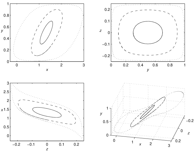
Figure 1: Integral lines of the velocity field for ${Re}=50$.

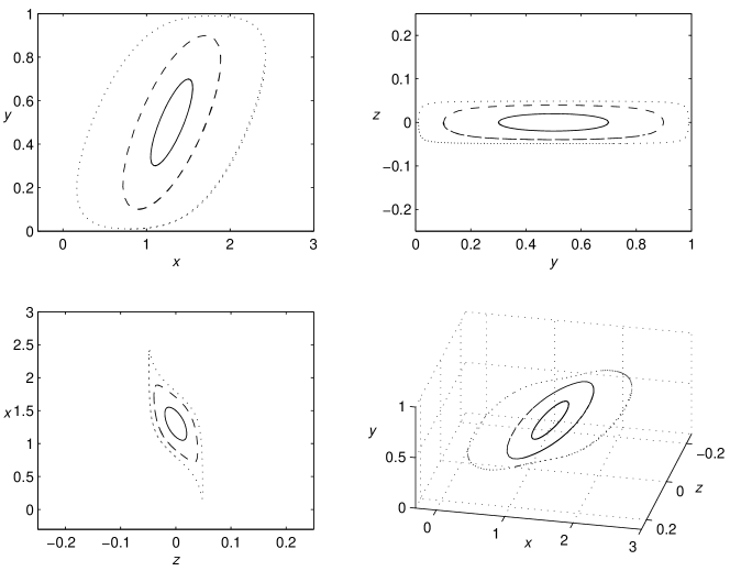
Figure 2: Integral lines of the velocity field for ${Re}=1000$.

As an example of the mini-max procedure, we show in Figure 3

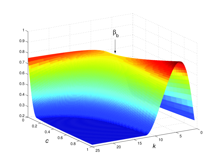
Figure 3: Bound on dissipation for $Re=50$ as a function of $c$ and $k$ (using $\Psi_{0.04}$).

the upper bound on the dissipation for $Re=50$ obtained by using as a test function $\Psi_{\delta}$ from (16raa) with $\delta=0.04$; the bound is given as a function of $c\in[0,1]$ and $k\in(0,25]$.

In Figure 4 we show the bound on the dissipation $\beta$ for $Re=50$ as a function of the balance parameter $c$ for different values of the span-wise wavenumber $k$; the data presented have been obtained with $\Psi_{\delta}$ with $\delta=0.04$.

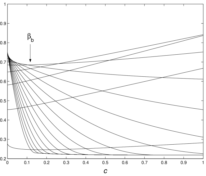
Figure 4: Bound on $\beta$ for $Re=50$ (obtained with $\Psi_{0.04}$) as a function of $c$ for several values of $k$.

The figure illustrates the general behavior of $\beta$ as a function of $k$ and $c$ – namely, for small $k$, the value of $\beta$ increases with $c$, while for larger $k$, $\beta$ decreases with $c$. Clearly, the family of lines in the figure has an envelope – this envelope is the graph of the function $\beta^{*}(50,0.04,c)$ (16ry). Having obtained the envelope, we find the minimum value of $\beta^{*}(50,0.04,c)$ – this is the mini-max value we are looking for; this point is labeled with $\beta_{b}$ in Figures 3 (where it is the saddle point) and 4.

4.2 Results

In Figure 5,

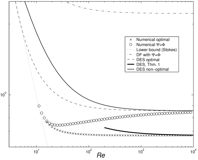
Figure 5: Upper and lower bounds on $\beta$.

we present the bounds from previous papers, as well as our new numerical results. The dotted straight line represents the lower limit on the dissipation corresponding to Stokes (laminar) flow,

$$\beta_{\mathrm{Stokes}}\geq\frac{\pi^{2}}{Re}\ .$$

The dot-dashed line in the upper part of the figure is the bound following [9] for this problem obtained with $\Psi=\Phi$:

$$\beta_{\mathrm{DF}}\leq\frac{\pi}{\sqrt{2}}+\frac{\pi^{2}}{Re}\ .$$

The thin solid line shows the “non-optimal” bound from [8] (equation (3.14) in [8]),

$$\beta_{\mathrm{DES,\ non-optimal}}\leq\frac{\sqrt{2}\pi}{\sqrt{27}}+\frac{\pi^{2}}{Re}\ ,$$

while the long-dashed one gives their “optimal” estimate (obtained from equation (3.12) in [8] by first minimizing over $\xi$ and then plugging $\Psi=\Phi$):

$$\beta_{\mathrm{DES,\ optimal}}\leq\frac{\sqrt{2}\pi}{\sqrt{27}}\left(1+\frac{2\pi^{2}}{3Re^{2}}\right)^{3/2}+\frac{\pi^{2}}{3Re}\left(1+\frac{4\pi^{2}}{9Re^{2}}\right)\ .$$

(Note that this line bifurcates from the lower Stokes bound at $Re=\sqrt{2}\pi\approx 4.4429$). The thick solid line starting from $Re\approx 178$ is the best upper bound for high values of $Re$ from Theorem 1 of [8]:

$$\beta_{\mathrm{DES,\ Thm.\ 1}}\leq\frac{\pi^{2}}{\sqrt{216}}+\frac{5(6\pi^{2})^{1/5}}{4^{4/5}\,Re^{4/5}}\approx 0.67154+\frac{3.73089}{Re^{4/5}}\ .$$ (16rab)

The circles in the figure give our new numerically determined upper bounds on $\beta$ with the choice $\Psi=\Phi$ and the crosses represent our numerical results for the choice (16raa) of $\Psi_{\delta}$.

In Figure 6 we have plotted

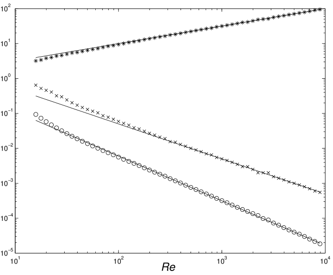
Figure 6: Power-law behavior of $\beta-\frac{\pi^{2}}{\sqrt{216}}$, $k^{*}$ and $c^{*}$ vs. ${Re}$ (see the text).

$\beta-\frac{\pi^{2}}{\sqrt{216}}$ (circles), $k^{*}$ (stars), and $c^{*}$ (x’s), versus $Re$ for the values of the dissipation bound obtained using the function $\Psi_{\delta}$ from (16raa). We see that $k^{*}\sim\sqrt{{Re}}$, $c^{*}\sim\frac{1}{{Re}}$, and from the figure we observe that $\beta-\frac{\pi^{2}}{\sqrt{216}}$ also behaves like a power of ${Re}$. In the figure we illustrate these behaviors by showing the straight lines

$$\beta=\frac{\pi^{2}}{\sqrt{216}}+\frac{2.158}{{Re}^{1.28}}\ ,\quad k^{*}=1.0\,\sqrt{{Re}}\ ,\quad c^{*}=\frac{5.0}{{Re}}\ .$$

5 Concluding remarks

We have derived new bounds on the energy dissipation rate for an example of body-force driven flow in a slippery channel. The fundamental improvement over previous results came from the application of the balance parameter in the variational formulation of the bounds, together with numerical solution of the Euler-Lagrange equations for the best estimate.

In Figure 7 the results of this analysis are compared with the direct

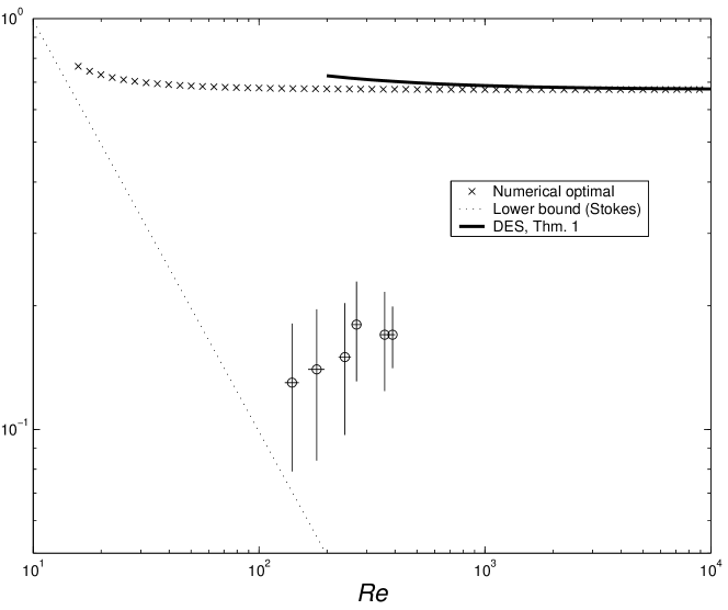
Figure 7: Comparison between theoretical results and DNS data (same symbols as in Figure 5).

numerical simulations of the three-dimensional Navier-Stokes equations first reported in [8]. Over the Reynolds number range 100–1000 where the data lie, the best bounds derived here, using the balance parameter and minimization over the (restricted) family of multiplier functions $\Psi_{\delta}$, result in a quantitative improvement over the previous rigorous estimates. We observe that the measured dissipation is a factor of 3 to 4 below the bound, which should be considered nontrivial given the a priori nature of the estimates derived here. Presumably a full optimization over possible multiplier functions $\Psi$ would result in a further lowering of the estimate at lower values of $Re$, producing a bound that intersects the lower Stokes bound right at the energy stability limit (which we compute to be at $Re=2\pi$). We note from Figure 5 that the bounds computed with $\Phi_{\delta}$ tend to agree with those computed using $\Phi=\Psi$ at lower values of $Re$, indicating that both trial functions are about the same “distance” from the true optimal multiplier.

At higher Reynolds numbers the optimal solutions computed here converge rapidly to the asymptotic bound $\beta_{b}(\infty)$ computed analytically in [9]. Indeed, the bound derived here approaches the asymptotic limit with a difference vanishing $\sim Re^{-1.28}$. This particular scaling of the approach to the asymptotic limit helps to understand the role that the balance parameter plays to lower the bound: while a naive estimate suggests that the approach might be ${\cal O}(Re^{-1})$, the faster convergence may be attributed to the interplay of the $c\sim Re^{-1}$ and $k\sim\sqrt{Re}$ scaling in the prefactor and the subtracted term in (12).

There are several directions in which this line of research could be continued. One is to develop more reliable and accurate analytical methods for estimating the best bounds at finite $Re$. This would probably involve asymptotic approximations for small but finite values of $Re^{-1}$ which could lead to more general applications for other variational problems as well. Another direction would be to develop methods to determine the true optimal multiplier function at finite $Re$. The motivation there would largely be as a point of principle, to demonstrate that the full min-max procedure can indeed be carried out—at least for simple set-ups such as those considered here. Finally, going beyond the simple $\sin{\pi y}$ forcing considered in this paper there remains the question, first posed in [8], as to the connection between the optimal multiplier and the true mean profile realized in direct numerical simulations. Specifically, the question is whether there is a sensible correspondence between the shape of the optimal multiplier and the mean profile for general force shapes. The idea is that the optimal multiplier contains information about the extreme fluctuations that might be realized in a turbulent flow, and some of those features may correlate with the statistical properties of the flows.

Appendix: Derivation of the expression (16rv) for $\Lambda$

In this Appendix we show how to derive the expression (16rv) for $\Lambda$ in the case $c=0$. First exclude $U$ from (16rc) with the help of (16ra):

$$\Lambda=\frac{\langle\Phi^{\prime}\Lambda\rangle\langle\Psi^{2}V^{2}\rangle}{\lambda^{2}\langle\Phi\Psi\rangle^{2}}\,\Phi^{\prime}-\frac{1}{Re}\,\frac{1}{\lambda\langle\Phi\Psi\rangle}\,\Bigl{(}\langle\Phi^{\prime}\Lambda\rangle\,\Psi^{\prime}+\langle\Psi^{\prime}\Lambda\rangle\,\Phi^{\prime}\Bigr{)}\ .$$ (16rac)

Now multiply the equation for $U$ (16ra) by $-U$, add it to the equation for $V$ (16rb) multiplied by $V$, and integrate the resulting identity to get the equidistribution property $\langle U^{2}\rangle=\left\langle V^{2}+\frac{1}{k^{2}}V^{\prime 2}\right\rangle$, so that the normalization condition (16q) can now be written as

$$2\left\langle V^{2}+\frac{1}{k^{2}}V^{\prime 2}\right\rangle+\langle\Lambda^{2}\rangle=1\ .$$ (16rad)

Multiplying (16rt) by $V$ and integrating using the boundary conditions (16rs), we obtain

$$\left\langle V^{2}+\frac{1}{k^{2}}V^{\prime 2}\right\rangle=\frac{E^{2}\langle\Psi^{2}V^{2}\rangle}{\langle\Psi^{2}\rangle}\ ,$$

which, together with the new normalization (16rad), yields

$$\frac{1-\langle\Lambda^{2}\rangle}{2}=\frac{E^{2}\langle\Psi^{2}V^{2}\rangle}{\langle\Psi^{2}\rangle}\ .$$

This expression and the definition of $E$ (16ru) allow us to write the coefficient of the term of order $Re^{0}$ in the right-hand side of (16rac) as

$$\frac{\langle\Phi^{\prime}\Lambda\rangle\langle\Psi^{2}V^{2}\rangle}{\lambda^{2}\langle\Phi\Psi\rangle^{2}}=\frac{E^{2}\langle\Psi^{2}V^{2}\rangle}{\langle\Psi^{2}\rangle\langle\Phi^{\prime}\Lambda\rangle}=\frac{1-\langle\Lambda^{2}\rangle}{2\langle\Phi^{\prime}\Lambda\rangle}\ .$$

Using the above relationship and expressing the Lagrange multiplier $\lambda$ from (16ru), we can rewrite (16rac) as

$$\Lambda=\left(\frac{1-\langle\Lambda^{2}\rangle}{2\langle\Phi^{\prime}\Lambda\rangle}-\frac{1}{Re}\,\frac{E}{\sqrt{\langle\Psi^{2}\rangle}}\,\frac{\langle\Psi^{\prime}\Lambda\rangle}{\langle\Phi^{\prime}\Lambda\rangle}\right)\,\Phi^{\prime}-\frac{1}{Re}\,\frac{E}{\sqrt{\langle\Psi^{2}\rangle}}\,\Psi^{\prime}\ .$$ (16rae)

Let $\mu$ be the coefficient of $\Phi^{\prime}$ in (16rae), i.e.,

$$\Lambda:=\mu\Phi^{\prime}-\frac{1}{Re}\,\frac{E}{\sqrt{\langle\Psi^{2}\rangle}}\,\Psi^{\prime}\ .$$ (16raf)

From this expression we easily obtain (recall that $\langle\Phi^{\prime 2}\rangle=1$)

$$\langle\Lambda^{2}\rangle = \mu^{2}-\frac{2E\langle\Phi^{\prime}\Psi^{\prime}\rangle}{Re\sqrt{\langle\Psi^{2}\rangle}}\,\mu+\frac{E^{2}\langle\Psi^{\prime 2}\rangle}{Re^{2}\langle\Psi^{2}\rangle}$$

$$\langle\Phi^{\prime}\Lambda\rangle = \mu-\frac{E\langle\Phi^{\prime}\Psi^{\prime}\rangle}{Re\sqrt{\langle\Psi^{2}\rangle}}$$

$$\langle\Psi^{\prime}\Lambda\rangle = \langle\Phi^{\prime}\Psi^{\prime}\rangle\,\mu-\frac{E\langle\Psi^{\prime 2}\rangle}{Re\sqrt{\langle\Psi^{2}\rangle}}\ .$$

Plugging these expressions in the definition of the coefficient $\mu$,

$$\mu=\frac{1-\langle\Lambda^{2}\rangle}{2\langle\Phi^{\prime}\Lambda\rangle}-\frac{1}{Re}\,\frac{E}{\sqrt{\langle\Psi^{2}\rangle}}\,\frac{\langle\Psi^{\prime}\Lambda\rangle}{\langle\Phi^{\prime}\Lambda\rangle}\ ,$$

we obtain the following quadratic equation for $\mu$:

$$3\mu^{2}-\frac{2E\langle\Phi^{\prime}\Psi^{\prime}\rangle}{Re\sqrt{\langle\Psi^{2}\rangle}}\,\mu-\left(1+\frac{E^{2}\langle\Psi^{\prime 2}\rangle}{Re^{2}\langle\Psi^{2}\rangle}\right)=0\ .$$

The “physical” solution of this equation (the one that has the right behavior in the limit $Re\to\infty$) is

$$\mu=-\frac{1}{\sqrt{3}}\,\sqrt{1+\frac{E^{2}}{Re^{2}\langle\Psi^{2}\rangle}\left(\langle\Psi^{\prime 2}\rangle+\frac{\langle\Phi^{\prime}\Psi^{\prime}\rangle^{2}}{3}\right)}+\frac{E\langle\Phi^{\prime}\Psi^{\prime}\rangle}{3Re\sqrt{\langle\Psi^{2}\rangle}}\ .$$

Plugging this into (16raf), we obtain the desired expression (16rv).

References

References

- [1] F. H. Busse. The optimum theory of turbulence. In Advances in Applied Mechanics, Vol. 18, pages 77–121. Academic Press, New York, 1978.
- [2] S. Childress, R. R. Kerswell, and A. D. Gilbert. Bounds on dissipation for Navier-Stokes flow with Kolmogorov forcing. Phys. D, 158(1-4):105–128, 2001.
- [3] P. Constantin and C. R. Doering. Variational bounds on energy dissipation in incompressible flows. II. Channel flow. Phys. Rev. E (3), 51(4, part A):3192–3198, 1995.
- [4] P. Constantin and C. R. Doering. Variational bounds on energy dissipation in incompressible flows. III. Convection. Phys. Rev. E (3), 53(6):5957–5981, 1996.
- [5] P. Constantin and C. R. Doering. Infinite Prandtl number convection. J. Statist. Phys., 94(1-2):159–172, 1999.
- [6] C. R. Doering and P. Constantin. Energy dissipation in shear driven turbulence. Phys. Rev. Lett., 69(11):1648–1651, 1992.
- [7] C. R. Doering and P. Constantin. Variational bounds on energy dissipation in incompressible flows: shear flow. Phys. Rev. E (3), 49(5, part A):4087–4099, 1994.
- [8] C. R. Doering, B. Eckhardt, and J. Schumacher. Energy dissipation in body-forced plane shear flow. J. Fluid Mech., 494:275–284, 2003.
- [9] C. R. Doering and C. Foias. Energy dissipation in body-forced turbulence. J. Fluid Mech., 467:289–306, 2002.
- [10] C. R. Doering and J. D. Gibbon. Applied Analysis of the Navier-Stokes Equations. Cambridge Texts in Applied Mathematics. Cambridge University Press, Cambridge, 1995.
- [11] C. R. Doering, E. A. Spiegel, and R. A. Worthing. Energy dissipation in a shear layer with suction. Phys. Fluids, 12(8):1955–1968, 2000.
- [12] C. R. Doering and X. Wang. Attractor dimension estimates for two-dimensional shear flows. Phys. D, 123(1-4):206–222, 1998. Nonlinear waves and solitons in physical systems (Los Alamos, NM, 1997).
- [13] C. Foias. What do the Navier-Stokes equations tell us about turbulence? In Harmonic Analysis and Nonlinear Differential Equations (Riverside, CA, 1995), volume 208 of Contemp. Math., pages 151–180. Amer. Math. Soc., Providence, RI, 1997.
- [14] C. Foias, O. Manley, R. Rosa, and R. Temam. Navier-Stokes Equations and Turbulence, volume 83 of Encyclopedia of Mathematics and its Applications. Cambridge University Press, Cambridge, 2001.
- [15] C. Foias, O. P. Manley, R. M. S. Rosa, and R. Temam. Cascade of energy in turbulent flows. C. R. Acad. Sci. Paris Sér. I Math., 332(6):509–514, 2001.
- [16] C. Foias, O. P. Manley, R. M. S. Rosa, and R. Temam. Estimates for the energy cascade in three-dimensional turbulent flows. C. R. Acad. Sci. Paris Sér. I Math., 333(5):499–504, 2001.
- [17] C. Foias, O. P. Manley, and R. Temam. Bounds for the mean dissipation of -D enstrophy and -D energy in turbulent flows. Phys. Lett. A, 174(3):210–215, 1993.
- [18] U. Frisch. Turbulence. Cambridge University Press, Cambridge, 1995. The legacy of A. N. Kolmogorov.
- [19] E. Hopf. Ein allgemeiner Endlichkeitssatz der Hydrodynamik. Math. Ann., 117:764–775, 1941.
- [20] L. N. Howard. Bounds on flow quantities. In Annual Review of Fluid Mechanics, Vol. 4, pages 473–494. Annual Reviews, Palo Alto, CA, 1972.
- [21] R. R. Kerswell. Unification of variational principles for turbulent shear flows: the background method of Doering-Constantin and the mean-fluctuation formulation of Howard-Busse. Phys. D, 121(1-2):175–192, 1998.
- [22] R. Nicodemus, S. Grossmann, and M. Holthaus. Improved variational principle for bounds on energy dissipation in turbulent shear flow. Phys. D, 101(1-2):178–190, 1997.
- [23] R. Nicodemus, S. Grossmann, and M. Holthaus. The background flow method. I. Constructive approach to bounds on energy dissipation. J. Fluid Mech., 363:281–300, 1998.
- [24] R. Nicodemus, S. Grossmann, and M. Holthaus. The background flow method. II. Asymptotic theory of dissipation bounds. J. Fluid Mech., 363:301–323, 1998.
- [25] J. Otero, L. Dontcheva, H. Johnston, R. A. Worthing, A. Kurganov, G. Petrova, and C. R. Doering. High-Rayleigh-number convection in a fluid-saturated porous layer. J. Fluid Mech., 500:263–281, 2004.
- [26] J. Otero, R. W. Wittenberg, R. A. Worthing, and C. R. Doering. Bounds on Rayleigh-Bénard convection with an imposed heat flux. J. Fluid Mech., 473:191–199, 2002.
- [27] K. R. Sreenivasan. On the scaling of the turbulence energy dissipation rate. Phys. Fluids, 27(5):1048–1051, 1984.
- [28] K. R. Sreenivasan. An update on the energy dissipation rate in isotropic turbulence. Phys. Fluids, 10(2):528–529, 1998.
- [29] L. N. Trefethen. Spectral Methods in MATLAB. Software, Environments, and Tools. SIAM, Philadelphia, PA, 2000.
- [30] J. A. C. Weideman and S. C. Reddy. A MATLAB differentiation matrix suite. ACM Trans. Math. Software, 26(4):465–519, 2000.