New experimental and theoretical approach to the 3d ²D-level lifetimes of ⁴⁰Ca⁺

Abstract

We report measurements of the lifetimes of the 3d ²D_5/2 and 3d ²D_3/2 metastable states of a single laser-cooled ⁴⁰Ca⁺ ion in a linear Paul trap. We introduce a new measurement technique based on high-efficiency quantum state detection after coherent excitation to the D_5/2 state or incoherent shelving in the D_3/2 state, and subsequent free, unperturbed spontaneous decay. The result for the natural lifetime of the D_5/2 state of 1168(9) ms agrees excellently with the most precise published value. The lifetime of the D_3/2 state is measured with a single ion for the first time and yields 1176(11) ms which improves the statistical uncertainty of previous results by a factor of four. We compare these experimental lifetimes to high-precision ab initio all order calculations and find a very good agreement. These calculations represent an excellent test of high-precision atomic theory and will serve as a benchmark for the study of parity nonconservation in Ba⁺ which has similar atomic structure.

I Introduction

The lifetime of the metastable D-levels in Ca⁺ is of high relevance in various experimental fields such as optical frequency standards, quantum information and astronomy. Trapped ion optical frequency standards Gill03 and optical clocks Diddams01 are based on narrow absorption lines in single laser-cooled ions. With transition linewidths in the 1 Hz range Rafac00 , Q-values (frequency of the absorption divided by its spectral width) of $\approx 10^{15}$ can be achieved. As the lifetimes of the D-levels in Ca⁺ are on the order of 1 s, yielding sub-Hz natural linewidths of the D-S quadrupole transitions, Ca⁺ has long been proposed as a promising candidate for a trapped ion frequency standard Werth89 . Such long lifetimes together with the ability to completely control the motional and electronic degrees of freedom of a trapped ion Leibfried03 make it ideally suited for storing and processing quantum information SasuraReview . In Ca⁺ a quantum bit (qubit) of information can be encoded within the coherent superposition of the S_1/2 ground state and the metastable D_5/2 excited state NaegerlQubit with very long coherence times FerdiCoherence ; RoosBell . In astronomy, absorption lines of Ca⁺ ions are used to explore the kinematics and structure of interstellar gas clouds Hobbs88 ; Welty96 and the D-level lifetimes are required for interpretation of the spectroscopic data. On the other hand, in theoretical atomic physics Ca⁺ is an excellent benchmark problem for atomic structure calculations owing to large higher-order correlation corrections and its similarity to Ba⁺. The size and distribution of the correlation corrections make it ideal for the study of the accuracy of various implementations of the all-order method. The properties of Ba⁺ are of interest due to studies of parity nonconservation in heavy atoms and corresponding atomic-physics tests of the Standard model of the electroweak interaction Koerber03 .

Figure 1: Ca⁺-level scheme with relevant transitions.

Experimental investigations of long atomic lifetimes have profited enormously from the development of ion trap technology and laser spectroscopy. Early experiments on the measurement of the D-level lifetimes in ⁴⁰Ca⁺ Urabe92 ; Arbes93 ; Arbes94 ; KnoopPRA95 ; Gudjons96 used large clouds of ions and the lifetime was determined by recovery of fluorescence on the UV-transitions (S_1/2 - P_1/2 or S_1/2 - P_3/2, see Fig. 1) after electron shelving in the D-states or by observing UV fluorescence after driving transitions from the D-states to the P-states. Shelving in this context means that the electron for a certain time remains in a metastable atomic level which is not part of a driven fluorescence cycle. These lifetime measurements were limited by deshelving induced by collisions with other ions or the buffer gas used for cooling. Similar results using the same techniques have been obtained in an ion storage ring Lidberg99 .

Much more accurate results can be obtained by performing lifetime measurements with single trapped ions Urabe93 ; Ritter97 ; Block99 ; Barton00 ; KnoopArxiv or strings of few trapped ions Staanum04 and employing the quantum jump technique. This technique is based on monitoring the fluorescence on the S_1/2 - P_1/2 dipole transition while at random times the ion is shelved to the metastable D_5/2-state where the fluorescence falls to the background level. For observing fluorescence both the S_1/2 - P_1/2 (397 nm) and the D_3/2 - P_1/2 (866 nm) transition have to be driven to prevent the ion from residing in the metastable D_3/2-state. Shelving to the D_5/2-state is initiated by applying laser light at 850 nm (D_3/2 - P_3/2) Urabe93 or at 729 nm (S_1/2 - D_5/2) KnoopArxiv . Statistical analysis of the fluorescence dark times yields the lifetime $\tau$. The most precise measurement using this technique was carried out by Barton et al. Barton00 who found the result of $\tau$=1168(7) ms.

Here, we introduce a measurement technique Kreuter04 based on deterministic coherent excitation to the D_5/2 state or incoherent shelving in the D_3/2 state, followed by a waiting period with free spontaneous decay and finally a measurement of the remaining excitation by high-efficiency quantum state detection. During the waiting time all lasers are shut off and no light interacts with the ion. This method basically is an improved version of a technique that was used earlier to measure the D_3/2 metastable level lifetime in single Ba⁺ ions Yu97 . The main advantage of this ”state detection” method is that no residual light is present during the measurement which could affect the free decay of the atom. In addition, it allows for the measurement of the D_3/2 level lifetime which otherwise is inaccessible with the quantum jump technique. There exist only a few reported D_3/2-level lifetime results for Calcium Arbes94 ; KnoopPRA95 ; Lidberg99 but none from a single ion experiment.

Figs. 2 and 3 compare the different experimental Urabe92 ; Arbes93 ; Urabe93 ; Arbes94 ; KnoopPRA95 ; Gudjons96 ; Ritter97 ; Lidberg99 ; Block99 ; Barton00 ; KnoopArxiv ; Staanum04 and theoretical Zeippen90 ; Guet91 ; Vaeck92 ; Brage93 ; Liaw95 ; Biemont96 methods and results for the D_5/2- and D_3/2-level lifetimes.

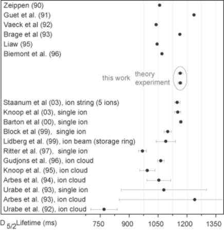
Figure 2: Theoretical and experimental results for the D_5/2-level lifetime.

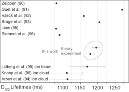
Figure 3: Theoretical and experimental results for the D_3/2-level lifetime.

From Fig. 2 it is evident that the single ion measurements are the most accurate ones. Generally, lifetime measurements on single ions or crystallized ion strings are more accurate as systematic errors, e.g. due to collisions, can be reduced to the highest possible extend. Therefore, single ion D-level lifetime measurements for Calcium are of special interest. The existence of accurate D-state lifetime values is of special interest for theory as well since most studies of alkali-metal atoms were focused on the measurements of the lowest $n$P-state lifetimes and D-states are much less studied. The properties of D-states are also generally more complicated to accurately calculate owing to large correlation corrections.

II Experimental Setup and Methods

For the experiments, a single ⁴⁰Ca⁺ ion is stored in a linear Paul trap in an ultra high vacuum (UHV) environment ($10^{-11}$ mbar range). The Paul trap is designed with four blades separated by 2 mm for radial confinement and two tips separated by 5 mm for axial confinement. Under typical operating conditions we observe radial and axial motional frequencies $(\omega_{\text{r1}},\omega_{\text{r2}},\omega_{\text{ax}})=2\pi(4.9,4.9,1.7)$ MHz. ⁴⁰Ca⁺ ions are loaded into the trap using a 2-step photoionization procedure GuldePhoto . The trapped ⁴⁰Ca⁺ ion has a single valence electron and no hyperfine structure (see Fig. 1). Doppler-cooling on the $\textrm{S}_{1/2}-\textrm{P}_{1/2}$ transition at 397 nm puts the ion in the Lamb-Dicke regime Leibfried03 ; SasuraReview . Diode lasers at 866 nm and 854 nm prevent optical pumping into the D states during cooling and state preparation. For coherent excitation to the D_5/2 state we drive the S_1/2 to D_5/2 quadrupole transition at 729 nm. A constant magnetic field of 3 G splits the 10 Zeeman components of the S_1/2 – D_5/2 multiplet. We detect whether a transition to D_5/2 has occurred by applying the laser beams at 397 nm and 866 nm and monitoring the fluorescence of the ion on a photomultiplier (PMT), i.e. using the electron shelving technique shelving . The internal state of the ion is discriminated with an efficiency close to 100$\%$ within approximately 3 ms Roos99 . The following stabilized laser sources are used in the experiment: two frequency-stabilized diode lasers at 866 nm and 854 nm with linewidths of $\approx$ 10 kHz and two Ti:Sa lasers at 729 nm ($<100$ Hz linewidth) and 794 nm ($<$ 100 kHz linewidth), of which the 794 nm laser is externally frequency doubled to obtain 397 nm. The experimental setup and the laser sources are described in more detail elsewhere FerdiCZReloaded ; NaegerlQubit .

III Measurement of the D_5/2 state lifetime

III.1 Measurement procedure and results

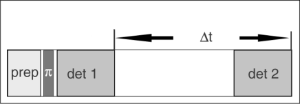
Figure 4: Simplified pulse scheme for the D_5/2 lifetime measurement: the preparation consists of Doppler cooling, repumping, and optical pumping (2ms); followed by a $\pi$-pulse (few $\mu$s) and a detection periods (3.5 ms). The waiting time is varied between 25 ms and 5 s.

The measurements consist of a repetition of laser pulse sequences applied to the ion. The sequence generally is composed of three steps (see Fig. 4):

1. State preparation and Doppler cooling, consisting of 2 ms of Doppler cooling (397 nm and 866 nm light), repumping from the D_5/2 level (854 nm light) and optical pumping into the S${}_{1/2}($m=-1/2$)$ Zeeman sublevel (397 nm $\sigma^{-}$ polarized light).

2. Coherent excitation at 729 nm with pulse length and intensity chosen to obtain near unity excitation ($\pi$-pulse) to the D${}_{5/2}(m=-5/2)$ Zeeman level.

3. State detection for 3.5 ms by recording the fluorescence on the S_1/2 - P_1/2 transition with a photomultiplier. Discrimination between S and D state is achieved by comparing the fluorescence count rate with a threshold value. The state is measured before and after a fixed waiting period $\Delta t$ to determine whether a decay of the excited state has happened.

This three-step cycle is repeated typically several thousand times. The decay probability $p$ is then determined as the ratio of D-state results in the second and the first state detections. For the calculation of the D_5/2-state lifetime $\tau_{(5/2)}$ we use an exponential fit function $(1-p)=\exp\{-\Delta t/\tau_{(5/2)}\}$. For $\Delta t$ we use the time interval between the ends of the two detection periods.

Fig. 5 shows the measured D_5/2-level excitation probability $(1-p)$ after several delay times ranging from 25 ms up to 5 s. A weighted least squares fit to the data yields the lifetime $\tau_{(5/2)}=1168(9)$ ms using the fitting function described above, where the only fitting parameter is $\tau_{(5/2)}$. The statistical error (in brackets) is the 1$\sigma$ standard deviation. The fit yields $\chi^{2}_{\nu}=0.47$, indicating that the experimental decay is consistent with the expected exponential decay behavior. The least-squares method is justified by the normal distribution of the mean decay probabilities which is a result of the ’central limit theorem’ of statistics. This was also verified using simulated data sets (see next section).

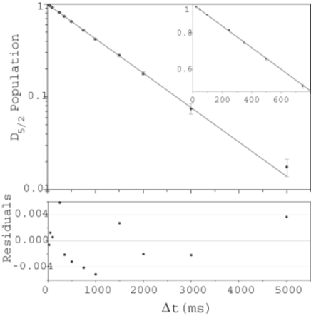
Figure 5: D_5/2-level excitation probability after delay times from 25 ms to 5 s plotted on a logarithmic scale. The solid line is a least squares fit to the data yielding $\tau_{\textrm{(5/2)}}=1168(9)$ ms. The residuals (difference of data points and fit curve) of the fit are shown in the lower diagram.

III.2 Systematic errors

There are several types of systematic errors that may affect the lifetime result. In UHV single ion experiments the biggest error source is usually radiation which irradiates the ion due to insufficient shielding of room light or insufficient shut-off of laser beams. In our experiment, the strongest influence stems from residual light at 854 nm. The influence of this radiation on the D_5/2 -level lifetime has been investigated extensively in Barton00 . If radiation at 854 nm is present during the delay interval it may de-excite the D_5/2-level to the ground state via the strongly coupled P_3/2-level. This additional ”decay channel” artificially shortens the observed lifetime. The obvious source for residual 854 nm radiation is the 854 nm diode laser itself. In our experiment, it is eliminated by a fast mechanical shutter Densitron which is closed during the delay interval. The 40 dB attenuation of the double-pass AOM which usually switches the 854 nm light was shown to be insufficient: In an earlier experiment without the shutter the lifetime was determined to 1011(6) ms FerdiCoherence . In addition, the results observed without shutter were found to fluctuate by approximately $\pm 50$ ms depending on the specific AOM and diode laser adjustments.

Another source for 854 nm radiation is background fluorescence at 854 nm from the 866 nm diode laser. To eliminate this radiation an AOM in single pass with an attenuation of more than 20 dB was used to shut the 866 nm beam. As the systematic lifetime error without AOM was found to be of the order of a few percent, this attenuation is sufficient. Note that this source of error cannot, in principle, be directly eliminated in the quantum-jump technique where 866 nm light must be radiated onto the ion continuously. In that case, the only way to correct for this systematic error is to measure at different light powers and extrapolate the lifetime to zero power which in turn implies a larger statistical error. In summary, radiation at 854 nm did not influence the measured D_5/2 -level lifetime at the given level of statistical uncertainty.

The D_5/2 -level lifetime could in principle be also reduced by transitions between the D-levels, i.e. by a M1-transition stimulated by thermal radiation. The corresponding transition rate is given by $W_{12}=B_{12}\rho(\nu)$ with the Einstein coefficient for stimulated emission $B_{12}$ and the energy density per unit frequency interval for thermal radiation $\rho(\nu)$. With the rate of spontaneous emission $A_{12}=(8\pi h\nu^{3}/c^{3})B_{12}$, $W_{12}$ is rewritten as:

$$W_{12}=\frac{A_{12}}{\textrm{e}^{h\nu/kT}-1}$$ (1)

With $\nu=1.82$ THz and $A_{12}=2.45\times 10^{-6}$ s^-1 taken from Ali88 we get $W_{12}=7.23\times 10^{-6}$ s^-1 at room temperature which changes the D_5/2 -level lifetime by much less than the statistical error of our measurement.

Residual radiation could also induce lifetime-enhancing systematic effects. Both radiation at 393 nm (roomlight) or 729 nm (Ti:Sa laser, double-pass AOM attenuation of $\approx 40$ dB) can lead to re-shelving of the ion. This effect, however, leads also to a different decay function. It is modeled by a simple rate equation for the excited state population $p_{D}$

$$\dot{p_{D}}=-\Gamma p_{D}+R(1-p_{D})$$ (2)

where $\Gamma=1/\tau$ denotes the natural decay rate and $R$ the reshelving rate induced by laser radiation. The solution of eq. (2) is of the form

$$p_{D}=A\textrm{e}^{-\Gamma^{\prime}t}+B$$ (3)

with $A=1-R/\Gamma^{\prime}$, an offset $B=R/\Gamma^{\prime}$ and the new decay rate $\Gamma^{\prime}=\Gamma+R$. Thus, an offset $B$ is the signature of a re-shelving rate. The result from fitting the experimental data in Fig. 5 with the modified exponential fit function (3) is $\tau_{\textrm{fit}}=1165(10)$ ms and $R_{\textrm{fit}}=3(2)\times 10^{-3}$ s^-1.

To evaluate the systematic error due to a repumping rate $R$ we use the following technique: We generate simulated data sets from random numbers by considering the fact that the decay probability for a given waiting time is distributed binomially around a mean that is given by an exponential function with an expected mean decay time $\tau_{(5/2)}$. For these data sets we also take into account the particular experimental waiting times and number of measurements. In this way ’ideal’ data sets are created that contain a purely statistical variation of data according to the experimental settings and that are free of any systematic errors. First, a fit of Eq. (3) to such an ideal simulated data set yields an additional repumping rate $R=0$ with a standard deviation of $\Delta R=3\times 10^{-3}$ s^-1. Thus, the above fitted repumping rate $R_{\textrm{fit}}$ is consistent with zero and not sufficiently significant to allow any conclusion about the actual rate or the model, i.e. the statistical error is too large for this small systematic error to be resolved in a fit to the data. Second, to obtain an upper limit for the systematic error of the lifetime due to a possible re-pumping rate we assume that such a rate $R_{\textrm{sim}}$ exists in the experiment. We then simulate data sets including the rate $R_{\textrm{sim}}$ and the lifetime $\tau_{(5/2)}$ and fit these data sets with a normal exponential fit function $(1-p)=\exp{(-\Delta t/\tau_{\textrm{sim}})}$. The deviation of the fit result $\tau_{\textrm{sim}}$ from $\tau_{(5/2)}$ used for the simulation gives the systematic lifetime error. For $R_{\textrm{sim}}=3\times 10^{-3}$ s^-1 this systematic error is $\Delta\tau=-3$ ms.

Another systematic effect that implies a different fit model is the state detection error. Even though the detection efficiency is close to unity, Poissonian noise in the PMT counts and the possibility of a spontaneous decay during the detection period produce a small error RoosPhD . The first error, i.e. the probability $\varepsilon_{1}$ to measure the ion in the wrong state due to noise of the count rate, depends on the discrimination between S and D state in the electron shelving technique. Such discrimination is achieved by comparing the fluorescence count rate during the detection window with a threshold value. Proper choice of this threshold value leads to an error as small as $\varepsilon_{1}=10^{-5}$ which can be neglected for the following analysis. The second error, i.e. the probability $\varepsilon_{2}$ for a wrong state measurement due to spontaneous decay, also depends on the length of the detection window, fluorescent count rates for the ion in S and D states and the threshold setting. For the chosen parameters in the experiment we evaluate $\varepsilon_{2}=10^{-3}$. The measured excitation probability is then $(1-p)_{\textrm{meas}}=(1-\varepsilon_{2})(1-p)_{\textrm{real}}$ and implies a model function of the form $(1-p)=(1-\varepsilon_{2})e^{-\Gamma\Delta t}$. A fit to simulated data as described above yields a statistically consistent limit for this detection error of $\varepsilon_{2}=1\times 10^{-3}$. Again, it cannot be resolved by a fit to the measured data. From simulated data including an assumed detection error of $\varepsilon_{2}=1\times 10^{-3}$ we get an upper limit of the systematic lifetime error $\Delta\tau=7$ ms.

In addition to radiative effects, non-radiative lifetime reduction mechanisms exist, namely, inelastic collisions with neutral atoms or molecules from the background gas. Two relevant types of collisions can be distinguished: Quenching and j-mixing collisions. Quenching collisions cause direct deshelving of the ion into the ground state. In the presence of high quenching rates lifetime measurements have to be done at different pressures. An extrapolation to zero pressure then yields the natural lifetime. Measurements of collisional deshelving rates for different atomic and molecular species have been performed in early experiments Arbes93 ; KnoopPRA95 . Ref. KnoopPRA95 finds specific quenching rates for Ca⁺ of $\Gamma_{H}^{q}=37\times 10^{-12}$ cm³s^-1 for H₂, and $\Gamma_{N}^{q}=170\times 10^{-12}$ cm³s^-1 for N₂. Collisions may also induce a change of the atomic polarization, a process called j-mixing or fine structure mixing where a transition from the D_5/2 to the D_3/2 state or vice versa is induced. These rates have also been determined in Ref.KnoopPRA95 to $\Gamma^{j}_{H}=3\times 10^{-10}$ cm³s^-1 for H₂ and $\Gamma^{j}_{N}=13\times 10^{-10}$ cm³s^-1 for N₂. Such collisional effects cannot be distinguished from a natural decay process. Collisional effects are most prominent in experiments with large clouds of ions or at higher background pressure. To give an upper limit of the effect in our experiment estimates of the constituents of the background gas must be made. If a background gas composition of 50% N₂ and 50% H₂ is assumed Aarhus and the pressure $p<2\times 10^{-11}$ mbar in the linear ion trap set up is taken into account, an upper limit for the additional collision induced rate of $\gamma=3\times 10^{-4}$ s^-1 is calculated. This effect is well below a $10^{-3}$ relative error and can be neglected here.

In summary, the result for the lifetime of the $D_{5/2}$ level can be quoted as: $\tau_{(5/2)}=1168$ ms $\pm 9$ ms (statistical) -3 ms (repumping rate) +7 ms (detection).

IV Measurement of the D_3/2 state lifetime

IV.1 Measurement procedure and results

For the measurement of the D_3/2-level lifetime some alterations in the pulse sequence are required (see Fig. 6). To populate the D_3/2 state we use indirect shelving by driving the S-P transition at 397 nm and taking advantage of the 1:16 branching ratio into the D_3/2 level. After a few microseconds the D_3/2 level is populated with unity probability.

Furthermore, because that level is part of the closed 3-level fluorescence cycle used for state detection its population cannot be probed with the state detection scheme described in the previous paragraph. In that sense the D_3/2 level is not a shelved state. The method used here is that prior to state detection the decayed population is transferred to the D_5/2 shelving state. The measured excitation probability of the D_5/2 state divided by the shelving probability then corresponds to the decay probability from the D_3/2 level and the further analysis is analogous to the one in Sec. III. Shelving in the D_5/2 state is achieved by coherent excitation ($\pi$-pulse). However, it must be taken into account that the D_3/2 state may decay into both Zeeman sublevels of the S_1/2 ground state. Hence, two $\pi$ pulses from both sublevels are required to transfer all decayed population to the D_5/2-state. In our experiment we chose the two $\Delta m_{j}=2$ transitions ($m_{j}=-1/2$ to $m_{j}=-5/2$ and $m_{j}=1/2$ to $m_{j}=5/2$). The combined transfer efficiency $P_{\pi}$ of the two pulses is determined in the first part of the pulse sequence (cf. Fig. 6): after Doppler cooling the ion is not optically pumped into the S${}_{1/2}(m_{j}=-1/2)$ ground state as usual but might populate both Zeeman sublevels. The measured transfer efficiency $P_{\pi}$ is used for calculation of the decay probability.

Figure 6: Simplified pulse scheme for the D_3/2 lifetime measurement. It consists of a measurement of the $\pi$-pulse transfer efficiency on the S_1/2-D_5/2 transition (prep, $\pi$ and det1); D_3/2-state preparation (prep, s); waiting period $\Delta t$ and state detection ($\pi$ and det2). For details of the pulse sequence see text. The waiting time is varied between 25 ms and 5 s.

The measurement of the D_3/2-level lifetime $\tau_{\textrm{(3/2)}}$ thus consists of a repetition of the following laser pulse sequences applied to the ion. The sequence generally is composed of three steps (cf. Fig. 6):

1. Measurement of transfer efficiency $P_{\pi}$: state preparation and Doppler cooling, consisting of 2 ms of Doppler cooling (397 nm and 866 nm light), repumping from the D_5/2 level (854 nm light) and spontaneous decay into the S${}_{1/2}($m=-1/2$)$ or $($m=+1/2$)$ Zeeman sublevel; $\pi$-pulses on the S_1/2 to D_5/2 transitions ($m_{j}=-1/2$ to $m_{j}=-5/2$ and $m_{j}=1/2$ to $m_{j}=5/2$); state detection for 3.5 ms by recording the fluorescence on the S_1/2 - P_1/2 transition with a photomultiplier.

2. State preparation and shelving in the D_3/2-level: 2 ms of Doppler cooling (397 nm and 866 nm light), repumping from the D_5/2 level (854 nm light) and optical pumping into the S${}_{1/2}($m=-1/2$)$ Zeeman sublevel (397 nm $\sigma^{-}$ polarized light); shelving pulse at 397 nm for a few $\mu$s.

3. Measurement of decay probability: free decay for a variable delay time; $\pi$-pulses on the S_1/2 to D_5/2 transitions ($m_{j}=-1/2$ to $m_{j}=-5/2$ and $m_{j}=1/2$ to $m_{j}=5/2$); state detection for 3.5 ms by recording the fluorescence on the S_1/2 - P_1/2 transition with a photomultiplier.

The measured D_3/2-level excitation probability $(1-p)$ is plotted vs. various delay times between 25 ms and 2 s in Fig. 7. Again, the data have been fitted using the least squares method and the fit function $1-p=\exp(-\Delta t/\tau_{\textrm{(3/2)}})$. Here, $p$ denotes the corrected decay probability $p=P_{ex}/P_{\pi}$, i.e. the detected excitation of the D_5/2 level $P_{ex}$ corrected for the near-unity shelving probability $P_{\pi}$ (which is typically 0.98-0.99 on average). Since there is no correlation between $P_{\pi}$ and $P_{ex}$ in one experiment it is more appropriate to use for the correction the average of $P_{\pi}$ for each delay time. The output from the fit is $\tau_{\textrm{(3/2)}}$ = 1176(11) ms with $\chi^{2}_{\nu}=0.68$ indicating good agreement of data and exponential model.

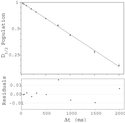
Figure 7: $D_{3/2}$-level excitation probability for delay times from 25 ms to 2 s plotted on a logarithmic scale. The solid line is a least squares fit to the data yielding $\tau_{\textrm{(3/2)}}$ = 1176(11) ms. The residuals (difference of data points and fit curve) of the fit are shown in the lower diagram.

IV.2 Systematic errors

Also for this experiment systematic errors due to residual light have to be investigated. The measured lifetime might be reduced by residual light at 866 nm or 850 nm present during the delay interval. This light would de-excite the D_3/2 level via the P_1/2- or P_3/2-levels, respectively, and results in a faster effective decay rate. The main source of light at 866 nm is the corresponding diode laser itself which is switched with a single pass AOM with an attenuation of 20 dB. As this attenuation was found to be insufficient a fast mechanical shutter (cf. Sec. III) was installed which remained closed throughout the entire waiting period. The fluorescence background of the 854 nm diode laser at 866 nm was found to be negligible. Light at 850 nm could de-shelve the ion via the P_3/2 state and is expected to mainly originate from the fluorescence background of the 854 nm diode laser. For this laser, a double-pass AOM attenuation of 40 dB was proven to be sufficient since no effect on the lifetime could be measured within a 5% error even if the laser was switched on at full intensity during the whole waiting time.

Lifetime reducing effects are not obviously detectable because they only increase the decay rate while the functional shape of the decay curve remains the same, i.e. no offset is introduced for long delay times. The main concern in our experiment is the 866 nm light and extreme care has been taken to ensure that the shutter was indeed closed during the delay time. Before the 397 nm shelving pulse and between the $\pi$ pulse and the second detection a 1 ms period has been inserted to allow for shutting time and jitter. During the lifetime measurements the correct shutting was checked by monitoring the transmission on photodiodes. In fact the shutters close fast within about 400 $\mu$s but the start time is not well defined and jitters by about 500 $\mu$s.

Lifetime prolonging effects can be induced by residual light at 397 nm or 729 nm which might re-excite the ion after it has already decayed. This re-shelving process can be detected as an offset as already pointed out in Sec. III. The 397 nm laser light is switched by two single pass AOM s in series (one before a fiber, one behind it, combined attenuation $\approx$ 55 dB). Nonetheless, we used a shutter to exclude the influence of 397 nm laser light to the largest possible extent. To give a limit on the systematic effect of any re-pumping source the same method as in section III.2 is applied. The experimental data is fitted with the rate model function Eq. (3) yielding a rate of $R_{\textrm{fit}}=3(10)\times 10^{-3}$ s^-1. The standard deviation of $R$ for an simulated ideal data set is $\Delta R=1.5\times 10^{-2}$ s^-1 (with mean $R=0$), so again the rate is concealed by the statistical error. From simulations an upper limit for the systematic lifetime error of $\Delta\tau=-2$ ms is obtained.

Another source of systematic error is vibrational heating of the ion during the delay time. If, due to heating, the transfer efficiency $P_{\pi}(\Delta t)$ is smaller after the waiting time than $P_{\pi}(0)$ determined in the first part of the pulse sequence the correction for the transfer efficiency is too small and the actual decay rate is higher than measured. A $\pi$ pulse only has high transfer efficiency if the ion is in the Lamb-Dicke regime Leibfried03 ; SasuraReview , i.e. $\eta^{2}\bar{n}<<1$ where $\eta$ is the Lamb-Dicke parameter and $\bar{n}$ is the mean phonon number. If the factor $\eta^{2}\bar{n}$ becomes significant both the Rabi frequency $\Omega_{\bar{n}}$ and the maximum transfer efficiency decrease as $\Omega_{\bar{n}}=\Omega_{0}(1-\eta^{2}\bar{n})$, where $\Omega_{0}$ is the coupling strength on the S-D transition. Taking the mean phonon number after Doppler cooling of $\bar{n}\approx 10$ and the measured heating rate in the linear ion trap of $\partial n/\partial t\approx 10$ s^-1 Roos99 we can estimate the transfer efficiency after a waiting time of 2 s, $P_{\pi}(2~{}\textrm{s})=0.98$ if the $\pi$-pulse time was initially chosen to fulfill $P_{\pi}(0)=1$. We experimentally checked the degradation of transfer efficiency with waiting time by introducing a delay time $\Delta t$ between the Doppler cooling pulse and the $\pi$-pulse in the first step of the pulse sequence and subsequently performing a state detection measurement. Figure 8 shows an average of various measurements of $\pi$-pulse transfer efficiency $P_{\pi}(\Delta t)$ vs. delay time $\Delta t$.

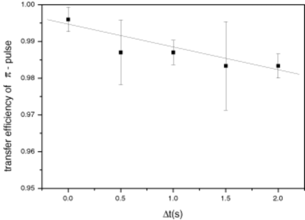
Figure 8: Average transfer efficiency of the $\pi$-pulses on the S_1/2 to D_5/2 transition after various delay times between Doppler cooling and $\pi$-pulses.

A linear fit $P_{\pi}(\Delta t)=1-a\Delta t$ to the data yields $a=-4(2)\times 10^{-3}$ s^-1. With simulated data sets including such a decreasing transfer efficiency $P_{\pi}(\Delta t)$ we determine a systematic lifetime error of $\Delta\tau=-7$ ms.

Finally, the detection error is considered, in analogy to section III.2. From simulated data sets with a detection error of $\varepsilon_{2}=1\times 10^{-3}$ a systematic error for the lifetime of $\Delta\tau=+8$ ms is found. Systematic errors due to collisional effects (quenching and j-mixing) can be again neglected as argued above.

Summarizing the analysis, the lifetime for the $D_{3/2}$ level is given as: $\tau_{\textrm{(3/2)}}=1176$ ms $\pm 11$ ms (statistical) -2 ms (repumping rate) -7 ms (heating) +8 ms (detection error).

V Ab initio all order calculation of the D-states lifetimes

We conducted the calculation of the 3d ²D_3/2 - 4s ²S_1/2 and 3d ²D_5/2 - 4s ²S_1/2 electric-quadrupole matrix elements in Ca⁺ using a relativistic all-order method which sums infinite sets of many-body perturbation theory terms. These matrix elements are used to evaluate the $3d$-level radiative lifetimes and their ratio.

In this particular implementation of the all-order method, the wave function of the valence electron $v$ is represented as an expansion

$$|\Psi_{v}\rangle = \left[1+\sum_{ma}\,\rho_{ma}a^{\dagger}_{m}a_{a}+\frac{1}{2}\sum_{mnab}\rho_{mnab}a^{\dagger}_{m}a^{\dagger}_{n}a_{b}a_{a}+\right.$$ (4)

$$+ \left.\sum_{m\neq v}\rho_{mv}a^{\dagger}_{m}a_{v}+\sum_{mna}\rho_{mnva}a^{\dagger}_{m}a^{\dagger}_{n}a_{a}a_{v}\right.$$

$$+ \left.\frac{1}{6}\sum_{mnrab}\rho_{mnrvab}a_{m}^{\dagger}a_{n}^{\dagger}a_{r}^{\dagger}a_{b}a_{a}a_{v}\right]|\Phi_{v}\rangle,$$

where $\Phi_{v}$ is the lowest-order atomic wave function, which is taken to be the frozen-core Dirac-Hartree-Fock (DHF) wave function of a state $v$. This lowest-order atomic wave function can be written as $|\Phi_{v}\rangle=a_{v}^{\dagger}|0_{C}\rangle,$ where $|0_{C}\rangle$ represents DHF wave function of a closed core. In equation (4), $a^{\dagger}_{i}$ and $a_{i}$ are creation and annihilation operators, respectively. The indices $m$, $n$, and $r$ designate excited states and indices $a$ and $b$ designate core states. The first two lines of Eq. (4) represent the single and double excitation terms. The restriction of the wave function to the first five terms of Eq. (4) represents a single-double (SD) approximation. The last term of Eq. (4) represents a class of the triple excitations and is included in the calculation partially as described in Ref. relsd . We carried out the all-order calculation with and without the partial addition of the triple term; the results of those two calculations are labeled SD (single-double) and SDpT (single-double partial triple) data in the text and tables below. The excitation coefficients $\rho_{ma}$, $\rho_{mv}$, $\rho_{mnab}$, and $\rho_{mnva}$ are obtained as the iterative solutions of the all-order equations in the finite basis set. The basis set, used in the present calculation, consists of the single-particle states, which are linear combinations of B-splines bsplines . The single-particle orbitals are defined on a non-linear grid and are constrained to a spherical cavity. The cavity radius is chosen to accommodate the $4s$ and $3d$ orbitals.

The matrix element of the operator $Z$ for the transition between the states $w$ and $v$ is obtained from the expansion (4) using

$$Z_{wv}=\frac{\langle\Psi_{w}|Z|\Psi_{v}\rangle}{\sqrt{\langle\Psi_{v}|\Psi_{v}\rangle\langle\Psi_{w}|\Psi_{w}\rangle}}.$$ (5)

The resulting expression for the numerator of the Eq. (5) consists of terms that are linear or quadratic functions of the excitation coefficients. We refer the reader to Refs. sd ; cs ; relsd for further description of the all-order method.

Table 1: Electric-quadrupole reduced matrix elements $E2$ in Ca⁺ (in a.u.) calculated using different approximations: Dirac-Hartree-Fock (DHF), third-order many-body perturbation theory (Third order), single-double all-order method (SD), and single-double all-order method including partial triple excitation contributions (SDpT). The all-order data calculated with $l_{\max}=6$ are listed separately. The contribution of basis set states with orbital angular momentum $l=7-10$ calculated using third-order MBPT is listed in rows labeled “Extr.”. This correction is added to obtain the values listed in rows labeled “SD” and “SDpT”.

Transition	Method	Value
3d 2D3/2 - 4s 2S1/2	DHF	9.767
	Third order	7.364
	SD${}_{l_{max}=6}$	7.788
	SDpT${}_{l_{max}=6}$	7.971
	Extr.	-0.038
	SD	7.750
	SDpT	7.934
3d 2D5/2 - 4s 2S1/2	DHF	11.978
	Third order	9.046
	SD${}_{l_{max}=6}$	9.562
	SDpT${}_{l_{max}=6}$	9.786
	Extr.	-0.046
	SD	9.516
	SDpT	9.740

Table 2: The Breit correction to the third-order values of the 4s ²S_1/2 - 3d ²D_3/2 and 4s ²S_1/2 - 3d ²D_5/2 electric-quadrupole matrix elements. The Dirac-Hartree-Fock values are given in column DHF. The random-phase approximation (RPA) values, iterated to all orders, are listed in column RPA. The third-order Brueckner-orbital, structure radiation, and normalization terms are listed in the columns BO, SR, and Norm, respectively.

Transition		DHF	RPA	BO	SR	Norm	Total
4s 2S1/2 - 3d 2D3/2	no Breit	9.7673	-0.0553	-2.2136	0.0621	-0.1588	7.4018
	with Breit	9.7611	-0.0552	-2.2131	0.0621	-0.1589	7.3961
	Difference	-0.0062	0.0001	0.0005	0.0000	-0.0001	-0.0057
4s 2S1/2 - 3d 2D5/2	no Breit	11.9782	-0.0662	-2.7006	0.0756	-0.1945	9.0926
	with Breit	11.9672	-0.0662	-2.7001	0.0756	-0.1946	9.0820
	Difference	-0.0110	0.0000	0.0005	0.0000	-0.0001	-0.0106

The numerical implementation of the all-order method requires to carry out the sums over the entire basis set. We truncate those sums at some value of the orbital angular momentum $l_{max}$; $l_{max}=6$ in the current all-order calculation. The contributions of the excited states with higher values of $l$ which are small but significant for the considered transitions, are evaluated in the third-order many-body perturbation theory (MBPT). To evaluate those contributions, we carried out a third-order MBPT calculation with the same basis set and $l_{max}$, used the all-order calculation and then repeated the third-order calculation with larger basis set containing the orbitals with $l$ up to $l_{max}=10$. The difference between these two results is added to the ab initio all-order results. The convergence of the MBPT terms with $l$ is rather rapid; the differences between the third-order calculations with $l_{max}=4,6,8,10$ are 1.8%, 0.4%, and 0.1%, respectively. The last number is well below the expected uncertainty of the current calculation. Thus, the contribution from orbitals with $l_{max}>10$ can be omitted at the present level of accuracy. The contribution from the excited states with $l_{max}>6$ relative to the total value of the matrix elements is significantly larger for $4s-3d$ electric-quadrupole transitions (about 0.5%) than for the primary $ns-np$ electric-dipole transitions in alkali-metal atoms. We note that while the all-order matrix elements contain the entire third-order perturbation theory contribution there is no straightforward and simple way to directly separate it out (see Ref. SafronovaPhD for the all-order vs. perturbation theory term correspondence issue). Thus, we have conducted a separate third-order calculation following Ref. ADNDT . The results of the third-order and the all-order calculations (with and without partial inclusion of the triple excitations) are listed in Table 1. The contribution from the excited states with orbital angular momentum $l>6$ calculated as described above is listed in the row labeled “Extr.”. The all-order values corrected for the truncation of the higher partial waves are listed in rows labeled “SD” and “SDpT”.

We also investigated the effect of the Breit interaction to the values of the electric-quadrupole matrix elements. The Breit interaction arises from the exchange of a virtual photon between atomic electrons. The static Breit interaction can be described by the operator

$$B_{ij}=-\frac{1}{r_{ij}}\hskip 2.84526pt\mbox{\boldmath$\alpha$}_{i}\cdot\mbox{\boldmath$\alpha$}_{j}+\frac{1}{2r_{ij}}\left[\hskip 2.84526pt\mbox{\boldmath$\alpha$}_{i}\cdot\mbox{\boldmath$\alpha$}_{j}-\left(\mbox{\boldmath$\alpha$}_{i}\cdot\mathbf{\hat{r}}_{ij}\right)\left(\mbox{\boldmath$\alpha$}_{j}\cdot\mathbf{\hat{r}}_{ij}\right)\right]$$ (6)

where the first part results from instantaneous magnetic interaction between Dirac currents and the second part is the retardation correction to the electric interaction shells . In Eq. (6), $\alpha$_i are Dirac matrices. The complete expression for the Breit matrix elements is given in breit . To calculate the correction to the matrix elements arising from the Breit interaction, we modified the generation of the B-spline basis set to intrinsically include the Breit interaction on the same footing as the Coulomb interaction and repeated the third-order calculation with the modified basis set. The difference between the new values and the original third-order calculation (conducted with otherwise identical basis set parameters) is taken to be the correction due to Breit interaction. We give the breakdown of the third-order calculation with and without inclusion of the Breit interaction in Table 2. The Dirac-Hartree-Fock values are given in column DHF. The random-phase approximation (RPA) values, iterated to all orders, are listed in column RPA. The third-order Brueckner-orbital, structure radiation and normalization terms are listed in the columns BO, SR, and Norm, respectively. The breakdown of the third-order calculation to RPA, BO, structure radiation and normalization terms follows that of Ref. ADNDT . The reader is referred to Ref. ADNDT for the detailed description of the third-order MBPT method and the formulas for all of the terms. We find the Breit correction to the DHF contribution to be dominant, with the contributions from all other terms being insignificant. The total Breit correction is very small and below the estimated uncertainty of our theoretical values discussed below. However, the Breit contribution to the ratio of the matrix elements is found to be small but significant owing to higher accuracy of the ratio.

The procedure described above does not include a class of the Breit correction contributions referred to in Ref. andrei_breit as two-body Breit contribution Breitfootnote . To conduct the study of the possible size of the two-body Breit contribution we calculated the Breit contribution to 10 different electric-dipole matrix elements ($6s-6p$, $6s-7p$, $7s-7p$, $7s-6p$, and $5d_{3/2}-6p$) in Cs using the method described above and compared those values with the results from andrei_breit . Cs is chosen as “model” atom as it is a similar system compared to Ca⁺. The Breit contribution to Cs properties was studied in detail owing to its importance for the interpretation of Cs parity nonconservation experiments. In Ref. andrei_breit , both one-body and dominant two-body Breit contributions have been taken into account. We find the largest difference between our data and that of andrei_breit to be 25%. For most of the transitions, we either agree to all the digits quoted in andrei_breit or differ by 10% or less. Therefore, the two-body contribution was not significant for any of the Cs electric-dipole transitions that we could compare with. We agree with the values of the Breit correction to the DHF matrix elements given in Ref. andrei_breit exactly, as expected, since the two-body Breit contribution only affects the correlation part of the calculation. Thus, we found no evidence that the two-body Breit correction may exceed the already calculated one-body correction, especially considering the fact that the Breit correction to the lowest-order DHF value dominates the one-body Breit correction to the $4s-3d$ matrix elements in Ca⁺. Therefore, we assume that the two-body Breit contribution does not exceed the already calculated part. In summary, the omission of the two-body Breit interaction introduces an additional uncertainty in our calculation and we take the uncertainty to be equal to the value of the correction itself. Most likely, it is an overly pessimistic assumption based on the comparison with the calculation of the Breit correction to Cs electric-dipole matrix elements carried out in Ref. andrei_breit .

Next, we use a semi-empirical scaling procedure to evaluate some classes of the correlation correction omitted by the current all-order calculation. The scaling procedure is described in Refs. cs ; SafronovaPhD . Briefly, the single-valence excitation coefficients $\rho_{mv}$ are multiplied by the ratio of the corresponding experimental and theoretical correlation energies and the calculation of the matrix elements is repeated with those modified excitation coefficients. This procedure is especially suitable in this particular study since the matrix element contribution containing the excitation coefficients $\rho_{mv}$ overwhelmingly dominates the correlation correction for the considered here transitions. We conduct this scaling procedure for both SD and SDpT calculations; the scaling factors are different in these two cases as SD method underestimates and SDpT method overestimates the correlation energy.

Table 3 contains the summary of the resulting matrix elements; the Breit correction is included in all values. We note that the scaled values only include DHF part of the Breit correction to avoid possible double counting of the terms (because of the use of the experimental correlation energy in the scaling procedure). The final values are taken to be scaled SD values based on the comparisons of similar calculations in alkali-metal atoms with experiment relsd ; SafronovaPhD ; rb . The uncertainty is calculated as the spread of the scaled values and ab initio SDpT values. The uncertainty in the Breit interaction calculation is also included; it is negligible in comparison with the spread of the values.

Table 3: Electric-quadrupole reduced matrix elements $E2$ in Ca⁺ (a.u.)

Transition	Method	ab initio	scaled
3d 2D3/2 - 4s 2S1/2	SD	7.744	7.939
	SDpT	7.928	7.902
	Final		7.939(37)
3d 2D5/2 - 4s 2S1/2	SD	9.505	9.740
	SDpT	9.729	9.694
	Final		9.740(47)

We use our final theoretical results to calculate the lifetimes of the D_3/2 and D_5/2 states in Ca⁺. The transition probabilities $A_{vw}$ are calculated using the formula WRJnotes

$$A_{vw}=\frac{1.11995\times 10^{18}}{\lambda^{5}}\frac{|\langle v\|Q\|w\rangle|^{2}}{2j_{v}+1}\,s^{-1},$$ (7)

where $\langle v\|Q\|w\rangle$ is the reduced electric-quadrupole matrix element for the transition between states $v$ and $w$ and $\lambda$ is corresponding wavelength in Å. The lifetime of the state $v$ is calculated as

$$\tau_{v}=\frac{1}{\sum_{w}A_{vw}}.$$ (8)

In both D_3/2 and D_5/2 lifetime calculations we consider a single transition contributing to each of the lifetimes. The transition probabilities of other transitions (M1 D_3/2 - S_1/2, M1 D_5/2 - D_3/2, and E2 D_5/2 - D_3/2) have been estimated in Ref. Ali88 and have been found to be 6 to 13 orders of magnitude smaller that the transition probabilities of the D_3/2 - S_1/2 and D_5/2 - S_1/2 E2 transitions. Thus, we neglect these transitions in the present study. The experimental energy levels from Ref. NIST are used in our calculation of the lifetimes. From the calculations we yield $\tau_{(3/2)}=1196(11)$ ms for the D_3/2-state and $\tau_{(5/2)}=1165(11)$ ms for the D_5/2-state. These lifetime values are compared with experimental and other theoretical results in Figs. 2 and 3.

Table 4: The ratio of the D_3/2 and D_5/2 lifetimes in Ca⁺ in various approximations. The lowest-order Dirac-Hartree-Fock results are labelled “DHF”, third-order many-body perturbation theory results are in column labelled “Third”, the results of the ab initio all-order calculation including single and double excitations are labeled “SD”, the results of the ab initio all-order calculation including single and double excitations with partial addition of the triple excitations are labeled “SDpT”, and the results of the corresponding scaled calculations are given in columns labeled “SD_sc” and “SDpT_sc”, respectively.

	DHF	Third	SD	SDpT	SDsc	SDpTsc	Final
No Breit	1.0251	1.0286	1.0275	1.0272	1.0266	1.0267
With Breit	1.0245	1.0278	1.0267	1.0265	1.0259	1.0260	1.0259(9)

The all-order calculation is in agreement with the present experimental values and recent experiments Barton00 ; KnoopArxiv ; Staanum04 within the uncertainty bounds. The present calculation includes the correlation correction, which is large (23%) for the considered transitions, in the most complete way with comparison to all other previous calculations Ali88 ; Zeippen90 ; Guet91 ; Vaeck92 ; Liaw95 and is expected to give the most accurate result. It is also the only calculation which gives an estimate of the uncertainty of the theoretical values.

In Ref. Barton00 , the issue of the theoretical ratio of the $\tau_{(3/2)}/\tau_{(5/2)}$ lifetimes was raised. It appeared that there was a disagreement between previously calculated theoretical ratios; Barton et al. Barton00 quotes the values 1.0283 Guet91 , 1.0175 Vaeck92 , and 1.0335 Liaw95 . Such a disagreement appears to be rather puzzling since this particular ratio is far less sensitive to the correlation correction than the values of the corresponding matrix elements. Thus, we studied the value of the ratio and its uncertainty in detail. We list the values of the ratio of the D_3/2 and D_5/2 lifetimes calculated in various approximations in Table 4. The experimental energy levels from Ref. NIST are used in all our calculations of the lifetimes for consistency. We include results with and without the addition of the Breit correction. As mentioned before, we find that the ratio does not change substantially with the addition of the correlation correction; in fact, the correlation only contributes about 0.15% to the final value. Thus, we calculate the uncertainty in the ratio by considering the spread of the high-precision values of the ratio itself (SD_sc, SDpT, and SDpT_sc), rather than calculating the uncertainty in the ratio from the uncertainties in the individual matrix elements. We also find that the while the Breit correction to the values of the matrix elements was insignificant at the current level of accuracy this is not the case for the ratio. In fact, the shift of the ratio values with the addition of the the Breit interaction is of the same order of magnitude as the spread of the high precision values as demonstrated in Table 4. We take the SD_sc value to be our final result for consistency with the calculation of the matrix elements. The uncertainty of the final value includes both the uncertainty in the correlation correction contribution and the uncertainty in the Breit interaction. As in the case of the individual matrix elements, the uncertainty in the Breit interaction is taken to be equal to the contribution itself. The Breit correction to the ratio is determined as the shift in the final ratio value due to addition of the Breit interaction.

Table 5: Comparison of the present values of the ratio of the D_3/2 and D_5/2 state lifetimes in Ca⁺ with other theory.

	Reference	Value
Theory	Ali88	1.03
	Zeippen90	1.02
	Guet91	1.028
	Vaeck92	1.02
	Liaw95	1.033
	Present	1.0259(9)
Expt.	Present	1.0068(122)

We compare our final theoretical value of the lifetime ratio with the experiment and other theory in Table 5. The ratios of the other theoretical values Ali88 ; Zeippen90 ; Guet91 ; Vaeck92 ; Liaw95 are calculated from the numbers in the original publications; care was taken to keep the number of digits in the ratio consistent with the number of digits in the values of the lifetimes or transitions rates quoted in the papers. First, we discuss the above mentioned discrepancy of the theoretical ratios. Ref. Barton00 lists the following ratios: 1.0283 Guet91 , 1.0175 Vaeck92 , and 1.0335 Liaw95 . We have listed the data from the original publications in Table 5 which shows that the actual numbers with taking into account the number of digits quoted in the original papers should have been 1271/1236=1.028 Guet91 , 1.16/1.14=1.02 Vaeck92 , and 1080/1045=1.033 Liaw95 . The first result is essentially a third-order relativistic many-body perturbation theory calculation with addition of semi-empirical scaling and omission of the some classes of small but significant third-order terms. It is very close to our third-order number 1.0286 from Table 4. The next paper Vaeck92 quotes only 3 digits in the lifetime values (1.16s and 1.14s) so the accuracy is insufficient to obtain the fourth digit in the ratio. We note that the method description in Vaeck92 is that of the non-relativistic calculation and it is unclear how the separation to D_3/2 and D_5/2 lifetimes was made. The last calculation yields a larger ratio but that calculation has serious numerical issues such as taking only 20 out of 40 B-splines and including too few partial waves. It also omits all terms except Brueckner-orbital ones and possibly even third-order Brueckner orbital contributions, which are large. The paper is not clear on the subject of the treatment of the higher-order contributions. Thus, we do not consider the result of Liaw95 to be reliable. Therefore, there are essentially no inconsistencies in the previously calculated theoretical ratios when the accuracy of the calculations is taken into account. Our theoretical value of the lifetime ratio is higher than the experimental value. The spread of all values in Table 5, including even lowest-order DHF values, is so small that it does not appear probable that any omitted Coulomb correlation or two-body Breit interaction can be responsible for the discrepancy. The only transition which can actually reduce the value of the theoretical ratio is the D_3/2-S_1/2 M1 transition. Thus, an accurate calculation of this transition rate will be useful in search for a theoretical explanation of the discrepancy. However, the transition rate published in Ali88 is extremely small ($A_{M1}=7.39\times 10^{-11}s^{-1}$) and has to be incorrect by many orders of magnitude to affect the ratio at such a level which does not appear likely since the same calculation gives a reasonably good (within 18%) number for the D_3/2-S_1/2 E2 transition rate.

VI Discussion

Figures 2 and 3 show an overview of the most recent experimental and theoretical results for the lifetime of the D_5/2 and D_3/2 states, respectively, in an chronological order. It is remarkable that the theoretical predictions scatter rather widely, with no noticeable convergence while the experimental results show a trend towards longer lifetimes in the recent years as more systematic errors are identified and stamped out.

In comparison with previous work it can be concluded here that our lifetime result for the D_5/2 level agrees with and thereby confirms the most precise value of Barton et al.. We stress that this lifetime measurement is an independent check of earlier results as we used a different measurement technique. In addition, the result for the D_3/2 level represents the first single ion measurement and reduces the statistical uncertainty of the previous values for the lifetime by a factor of four.

For the calculated lifetimes we find excellent agreement of the theoretical all-order lifetimes with the experimental results. Such agreement demonstrates the necessity of including partially the triple contributions to the all-order calculations for these types of transitions and confirms that scaling of the single-double all-order results, which is significantly simpler and less time consuming calculation in comparison with ab initio inclusion of partial triple excitations, is adequate for these types of transitions. This is an important result for the evaluation of the accuracy of similar theoretical calculation in Ba⁺ which is important to parity violating experiments in heavy atoms. Such experiments are aimed at the tests of the Standard model of the electroweak interaction and at the study of the nuclear anapole moments. One of the features of most PNC studies in heavy atoms is the need for comparable accuracy of theoretical and experimental data. The current study is also of interest in regard to recently found discrepancy between the $5d$ lifetimes and the $6s-6p$ Stark shifts in Cs uscs . Atomic properties of cesium were studied extensively by both experimentalists and theorists owing to a high-precision measurement of parity non-conserving amplitude in this atom. Both of these quantities depend on the values of the $5d-6p$ matrix elements. While those matrix elements are the electric-dipole ones rather than the electric-quadrupole ones studied here, the calculation itself as well as the breakdown of the correlation correction terms is very similar to the present calculation. Thus, the current study presents an important benchmark in the field of high-precision measurements and calculations. The study of the lifetime ratio demonstrated that the Breit interaction, which produces only a very small correction to the values of the actual matrix elements, is important in high-precision calculations of the corresponding matrix element ratios.

VII Acknowledgements

This work is supported by the Austrian ’Fonds zur Förderung der wissenschaftlichen Forschung’ (SFB15), by the European Commission: IHP network ’QUEST’ (HPRN-CT-2000-00121), Marie Curie Research Training network ’CONQUEST’ (MRTN-CT-2003-505089) and IST/FET program ’QUBITS’ (IST-1999-13021), and by the ”Institut für Quanteninformation GmbH”. C. Russo acknowledges support by Fundação para a Ciência e a Tecnologia (Portugal) under the grant SFRH/BD/6208/2001. H. H. is funded by the Marie-Curie-program of the European Union.

References

- (1) P. Gill, G.P. Barwood, H.A. Klein, G. Huang, S.A. Webster, P.J. Blythe, K. Hosaka, S.N. Lea, and H.S. Margolis, Meas. Sci. Technol. 14, 1174 (2003).
- (2) S.A. Diddams, T. Udem, J.C. Bergquist, E.A. Curtis, R.E. Drullinger, L. Hollberg, W.M. Itano, W.D. Lee, C.W. Oates, K.R. Vogel, and D.J. Wineland, Science 293, 825 (2001).
- (3) R.J. Rafac, B.C. Young, J.A. Beall, W.M. Itano, D.J. Wineland, and J.C. Bergquist, Phys. Rev. Lett. 85, 2462 (2000).
- (4) G. Werth in Applied Laser Spectroscopy (eds. W. Demtröder and M. Inguscio), NATO ASI Series B, Vol. 241, 479, (Plenum Press, New York, 1990).
- (5) D. Leibfried, R. Blatt, C. Monroe, and D.J. Wineland, Rev. Mod. Phys. 75, 281 (2003).
- (6) M. Šašura and V. Bužek, J. Mod. Opt. 49, 1593 (2002)
- (7) H.C. Nägerl, Ch. Roos, D. Leibfried, H. Rohde, G. Thalhammer, J. Eschner, F. Schmidt-Kaler, R. Blatt: Phys. Rev. A 61, 023405 (2000)
- (8) F. Schmidt-Kaler, S. Gulde, M. Riebe, T. Deuschle, A. Kreuter, G. Lancaster, C. Becher, J. Eschner, H. Häffner, and R. Blatt, J. Phys. B: At. Mol. Opt. Phys. 36, 623 (2003)
- (9) C.F. Roos, G.P.T. Lancaster, M. Riebe, H. Häffner, W. Hänsel, S. Gulde, C. Becher, J. Eschner, F. Schmidt-Kaler, and R. Blatt, Phys. Rev. Lett. 92, 220402 (2004).
- (10) L.M. Hobbs, A.M. Lagrange-Henri, R. Ferlet, A. Vidal-Madjar, and D.E. Welty, Astrophys. J. 334, L41 (1988).
- (11) D.E. Welty, D.C. Morton, and L.M. Hobbs, Astrophys. J. 106, 533 (1996).
- (12) T.W. Koerber, M.H. Schacht, W. Nagourney, and E.N. Fortson, J. Phys. B. 36, 637 (2003).
- (13) S. Urabe, M. Watanabe, H. Imajo, and K. Hayasaka, Opt. Lett. 17, 1140 (1992).
- (14) F. Arbes, T. Gudjons, F. Kurth, G. Werth, F. Marin, and M. Inguscio, Z. Phys. D 25, 295 (1993).
- (15) F. Arbes, M. Benzing, T. Gudjons, F. Kurth, and G. Werth, Z. Phys. D 29, 159 (1994).
- (16) M. Knoop, M. Vedel, and F. Vedel, Phys. Rev. A 52, 3763 (1995).
- (17) T. Gudjons, B. Hilbert, P. Seibert, and G. Werth, Europhys. Lett. 33, 595 (1996).
- (18) J. Lidberg, A. Al-Khalili, L.-O. Norlin, P. Royen, X. Tordoir, and S. Mannervik, J. Phys. B: At. Mol. Opt. Phys. 32, 757 (1999).
- (19) S. Urabe, K. Hayasaka, M. Watanabe, H. Imajo, R. Ohmukai, and R. Hayashi, Appl. Phys. B 57, 367 (1993).
- (20) G. Ritter and U. Eichmann, J. Phys. B: At. Mol. Opt. Phys. 30, L141 (1997).
- (21) M. Block, O. Rehm, P. Seibert, and G. Werth, Eur. Phys. J. D 7, 461 (1999).
- (22) P.A. Barton, C.J.S. Donald, D.M. Lucas, D.A. Stevens, A.M. Steane, and D.N. Stacey, Phys. Rev. A 62, 032503 (2000).
- (23) M. Knoop, C. Champenois, G. Hagel, M. Houssin, C. Lisowski, M. Vedel, and F. Vedel, Eur. Phys. J. D 29, 163 (2004).
- (24) P. Staanum, I.S. Jensen, R.G. Martinussen, D. Voigt, and M. Drewsen, Phys. Rev. A 69, 32503 (2004).
- (25) A. Kreuter, C. Becher, G.P.T. Lancaster, A.B. Mundt, C. Russo, H. Häffner, C. Roos, J. Eschner, F. Schmidt-Kaler, and R. Blatt, Phys. Rev. Lett. 92, 203002 (2004).
- (26) N. Yu, W. Nagourney, and H. Dehmelt, Phys. Rev. Lett. 78, 4898 (1997).
- (27) C.J. Zeippen, Astron. Astrophys. 229, 248 (1990).
- (28) C. Guet and W.R. Johnson, Phys. Rev. A 44, 1531 (1991).
- (29) N. Vaeck, M. Godefroid, and C. FroeseFischer, Phys. Rev. A 46, 3704 (1992).
- (30) T. Brage, C. Froese-Fischer, N. Vaeck, M. Godefroid, and A. Hibbert, Physica Scripta 48, 533 (1993).
- (31) S.S. Liaw, Phys. Rev. A 51, R1723 (1995).
- (32) E. Biemont and C.J. Zeippen, Comments At. Mol. Phys. 33, 29 (1996).
- (33) S. Gulde, D. Rotter, P. A. Barton, F. Schmidt-Kaler, and R. Blatt, Appl. Phys. B 73, 861 (2001).
- (34) H. Dehmelt: Bull. Am. Phys. Soc. 20, 60 (1975); W. Nagourney, J. Sandberg, and H. Dehmelt, Phys. Rev. Lett. 56, 2797 (1986); Th. Sauter, W. Neuhauser, R. Blatt, and P. E. Toschek, ibid 57, 1696 (1986); J. C. Bergquist, R. G. Hulet, W. M. Itano, D. J. Wineland, ibid 57, 1699 (1986).
- (35) Ch. Roos, Th. Zeiger, H. Rohde, H.C. Nägerl, J. Eschner, D. Leibfried, F. Schmidt-Kaler, and R. Blatt, Phys. Rev. Lett. 83, 4713 (1999).
- (36) F. Schmidt-Kaler, H. Häffner , S. Gulde, M. Riebe, G.P.T. Lancaster, T. Deuschle, C. Becher, W. Hänsel, J. Eschner, C.F. Roos, and R. Blatt, Appl. Phys. B 77, 789 (2003).
- (37) Densitron, TK-CMD series. Using suitable electronics for the shutter drive, closing and opening times of the order of 0.5 ms can be achieved. The timing jitter is on the same time scale.
- (38) M.A. Ali and Y.K. Kim, Phys. Rev. A 38, 3992 (1988).
- (39) C. Roos, Ph.D. thesis, University of Innsbruck (2000).
- (40) Assumption based on the mass spectrometer analysis in the Aarhus ion trap experiment Staanum04 .
- (41) M.S. Safronova, W.R. Johnson, and A. Derevianko, Phys. Rev. A 60, 4476 (1999).
- (42) W.R. Johnson, S.A. Blundell, and J. Sapirstein, Phys. Rev. A 37, 307 (1998).
- (43) S.A. Blundell, W.R. Johnson, Z.W. Liu, and J. Sapirstein, Phys. Rev. A 40, 2233 (1989).
- (44) S.A. Blundell, W.R. Johnson, and J.Sapirstein, Phys. Rev. A43, 3407 (1991).
- (45) M.S. Safronova, Ph.D. thesis, University of Notre Dame (2000).
- (46) W.R. Johnson, Z.W. Liu, and J. Sapirstein, At. Data and Nucl. Data Tables 64, 279 (1996).
- (47) W.R. Johnson and K. T. Cheng, in Atomic Inner-Shell Physics, edited by B. Crasemann (Plenum press, New York, 1985), pp. 3-30.
- (48) W.R. Johnson, S.A. Blundell, and J. Sapirstein, Phys. Rev. A 37, 2764 (1998).
- (49) A. Derevianko, Phys. Rev. A 65, 012106 (2002).
- (50) The Breit interaction is a two-particle interaction just as the Coulomb interaction. The separation of the Breit contribution to “one-body” and “two-body” parts results from transforming the Breit operator in second quantization to normal form as described in Ref. andrei_breit .
- (51) M.S. Safronova, C.J. Williams, and C.W. Clark, Phys. Rev. A 69, 022509 (2004).
- (52) W.R. Johnson, Lecture Notes on Atomic Physics, http://www.nd.edu/~johnson
- (53) NIST Atomic Spectra Database Available online: http://physics.nist.gov/cgi-bin/AtData/main_asd
- (54) M.S. Safronova and C.W. Clark, Phys. Rev. A 69, 040501 (2004).