Contactless inductive flow tomography

Abstract

The three-dimensional velocity field of a propeller driven liquid metal flow is reconstructed by a contactless inductive flow tomography (CIFT). The underlying theory is presented within the framework of an integral equation system that governs the magnetic field distribution in a moving electrically conducting fluid. For small magnetic Reynolds numbers this integral equation system can be cast into a linear inverse problem for the determination of the velocity field from externally measured magnetic fields. A robust reconstruction of the large scale velocity field is already achieved by applying the external magnetic field alternately in two orthogonal directions and measuring the corresponding sets of induced magnetic fields. Kelvin’s theorem is exploited to regularize the resulting velocity field by using the kinetic energy of the flow as a regularizing functional. The results of the new technique are shown to be in satisfactory agreement with ultrasonic measurements.

I Introduction

Flow measurement in metallic and semiconducting melts is a notorious problem in a number of technologies, reaching from iron casting to silicon crystal growth. Obviously, the usual optical methods of flow measurement are inappropriate for those opaque fluids. Ultrasonic techniques have problems, too, when applied to very hot or chemically aggressive melts. A completely contactless flow measurement technique would be highly desirable, even if it were only to provide a rough picture of the flow.

Fortunately, metallic and semiconducting melts are characterized by a high electrical conductivity. Hence, when exposed to an external magnetic field, the flowing melt gives rise to electrical currents that lead to a deformation of the applied magnetic field. This field deformation is measurable outside the fluid volume, and it can be used to reconstruct the velocity field, quite in parallel with the well-known magnetoencephalography, where neuronal activity in the brain is inferred from magnetic field measurements HAEM . The goal of this paper is to report on a first experimental demonstration of such a contactless inductive flow tomography (CIFT).

II Theory

The ratio of the induced field to the applied field is determined by the so-called magnetic Reynolds number, defined as $Rm=\mu\sigma vl$, with $\mu$ denoting the magnetic permeability of the melt, $\sigma$ its electrical conductivity, $v$ a typical velocity, and $l$ a typical length scale of the flow. In industrial applications, $Rm$ is in the order of 0.01…1. Only for a few large scale sodium flows, as they appear in fast breeder reactors, but also in the recent hydromagnetic dynamo experiments RMP , $Rm$ reaches values in the order of 10…100 (of course, in some cosmic dynamos $Rm$ can be even much larger). Actually, the present work was strongly motivated by the wish to reconstruct the sodium flow in the Riga dynamo experiment by an appropriate contactless method.

Suppose the fluid to flow with the stationary velocity $\bf v$, and to be exposed to a magnetic field ${\bf B}$, which we leave unspecified for the moment. Then, according to Ohms law in moving conductors the current

$$\bf{j}=\sigma(\bf{v}\times{\bf{B}}-\nabla\varphi)$$ (1)

is induced, with $\varphi$ denoting the electric potential. This current gives rise to the induced magnetic field

$${\bf{b}}({\bf{r}}) = \frac{\mu_{0}\sigma}{4\pi}\iiint_{V}\frac{({\bf{v}}({\bf{r^{\prime}}})\times{\bf{B}}({\bf{r^{\prime}}}))\times({\bf{r}}-{\bf{r^{\prime}}})}{|{\bf{r}}-{\bf{r^{\prime}}}|^{3}}\;dV^{\prime}$$ (2)

$$-\frac{\mu_{0}\sigma}{4\pi}\oiint_{S}\varphi({\bf{s^{\prime}}}){\bf{n}}({\bf{s^{\prime}}})\times\frac{{\bf{r}}-{\bf{s^{\prime}}}}{|{\bf{r}}-{\bf{s^{\prime}}}|^{3}}\;dS^{\prime}\;.$$

Equation (2) follows from inserting Eq. (1) into Biot-Savart’s law and transforming the volume integral over $\nabla\varphi$ into a surface integral over $\varphi$.

The electric potential $\varphi$ at the boundary $S$, in turn, has to fulfill the boundary integral equation

$$\varphi({\bf{s}}) = \frac{1}{2\pi}\iiint\limits_{D}\frac{({\bf{v}}({\bf{r^{\prime}}})\times{\bf{B}}({\bf{r^{\prime}}}))\cdot({\bf{s}}-{\bf{r^{\prime}}})}{|{\bf{s}}-{\bf{r^{\prime}}}|^{3}}\;dV^{\prime}$$ (3)

$$-\frac{1}{2\pi}\oiint\limits_{S}\varphi({\bf{s^{\prime}}}){\bf{n}}({\bf{s^{\prime}}})\cdot\frac{{\bf{s}}-{\bf{s^{\prime}}}}{{|{\bf{s}}-{\bf{s^{\prime}}}|}^{3}}\;dS^{\prime}\;.$$

Equation (3) follows from taking the divergence of Eq. (1) and utilizing $\nabla\cdot{\bf j}=0$. Then, Green’s theorem can be applied to the solution of the arising Poisson equation $\Delta\varphi=\nabla\cdot({\bf{v}}\times{\bf{B}})$, with demanding that the current is purely tangential at the boundary INV1 . Note that Eq. (3) is the basic formula for the vast area of electric inductive flow measurement SHER which is, however, not the subject of the present work.

In general, the magnetic field $\bf B$ on the right hand sides of Eqs. (1-3) is the sum of an externally applied magnetic field ${\bf B}_{0}$ and the very induced magnetic field $\bf b$. Hence Eqs. (2,3) represent an integral equation system which actually can be used to solve dynamo problems in arbitrary bounded domains XU . It it also suitable for a systematic investigation of the non-linear induction effects as they appear already in the sub-critical regime of laboratory dynamos VKS .

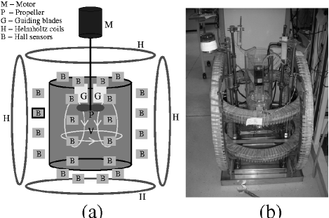
Figure 1: Scheme (a) and photograph (b) of the CIFT experiment.

In the following, however, all considerations will be restricted to problems with small $Rm$ for which $\bf B$ can be replaced by ${\bf B}_{0}$. Then, we get a linear relation between the desired velocity field and the induced magnetic field which is supposed to be measured. But how to cope with the remaining Eq. (3) for the electric potential?

Figure 2: Propeller rotation rate, and induced magnetic field measured at the Hall sensor emphasized in Fig. 1a.

The answer to this question can be adopted from magnetoencephalography HAEM . Assume, for a given ${\bf B}_{0}$, all measured magnetic field data be collected into an $N_{B}$ dimensional vector with the entries $b^{(B_{0})}_{i}$, and the desired velocity components at the $N_{V}$ discretization points by a vector with the entries $v_{n}$. The solution of the boundary integral equation may require a fine discretization of the boundary, with $N_{P}$ degrees of freedom $\varphi^{(B_{0})}_{k}$. Eqs. (2,3) can then be written in the form

$$b^{(B_{0})}_{i} = R^{(B_{0})}_{in}v_{n}+S_{ik}\varphi^{(B_{0})}_{k}$$ (4)

$$\varphi^{(B_{0})}_{k} = T^{(B_{0})}_{kn}v_{n}+U_{kk^{\prime}}\varphi^{(B_{0})}_{k^{\prime}}\;,$$ (5)

where the matrices ${\bf{R}}^{(B_{0})}$ and ${\bf{T}}^{(B_{0})}$ depend on the applied field ${\bf B}_{0}$, whereas the matrices $\bf S$ and $\bf U$ depend only on geometric factors.

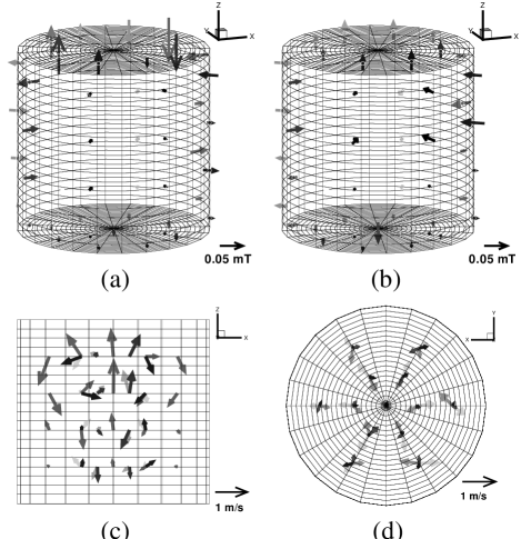
Figure 3: Measured induced magnetic field components for transverse (a) and axial (b) applied magnetic field, and reconstructed velocity as seen from the side (c) and from below (d). The grey scale of the arrows indicates the distance from the eye. The propeller pumps upward with 1200 rpm.

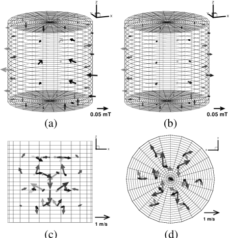
Figure 4: The same as Fig. 3, but for the propeller pumping downward with 1200 rpm.

As is well known from magnetoencephalography, the inversion of Eq. (5) is a bit tricky due to the singularity of the matrix $({\bf{I}}-{\bf{U}})$. This singularity mirrors the fact that the electric potential is defined only up to an additive constant. We can remove this ambiguity by replacing $({\bf{I}}-{\bf{U}})$ by a generally well conditioned matrix $({\bf{I}}-{\bf{U}})^{defl}:=({\bf{I}}-{\bf{U}})-N^{-1}{\bf e}{\bf e}^{T}$, where ${\bf e}$ is a vector with all $N$ entries equal to one and ${\bf e}^{T}$ is its transposed. By applying this so-called deflation method HAEM one ends up with

$$b^{(B_{0})}_{i} = R^{(B_{0})}_{in}v_{n}+S_{ik^{\prime}}(I-U)^{-1,defl}_{k^{\prime}k}T^{(B_{0})}_{kn}v_{n}\;,$$ (6)

i.e., with a linear relation between the desired velocity field and the measured magnetic field.

Figure 5: Tikhonov’s L-curve for the two different pumping directions. The arrows point at the bended knee where the curves have the strongest curvature. At these points we get a reasonable compromise between data fitting and minimum kinetic energy of the modelled velocity field. The rms of these velocities is approximately 0.41 m/s for the upward pumping and 0.73 m/s for the downward pumping.

Despite the far-reaching similarity, there is one essential difference of our method compared to magnetoencephalography. While in the latter one has to determine a single neuronal current distribution, in our case we can produce quite different current distributions from the same flow field simply by applying various external magnetic fields subsequently. For each applied magnetic field we can measure the corresponding induced fields, and utilize all of them to reconstruct the flow.

Concerning the uniqueness question for this sort of inversion, here we give only a shortened answer, referring for more details to the previous papers INV2 ; MEAS . For spherical geometry, and the two applied magnetic fields pointing in orthogonal directions, the problem can be solved with some rigour. Suppose we have measured the two corresponding sets of induced magnetic fields on a sphere outside the fluid volume, and have expanded them into spherical harmonics. The desired (solenoidal) velocity field can be represented by two scalars for its poloidal and toroidal parts. These two scalars can also be expanded into spherical harmonics, but with the expansion coefficient still being functions of the radius. In MEAS it had been shown (at least in some low degrees of the spherical harmonics expansion) that what can be derived from the two magnetic field expansion coefficients are some radial moments of the expansion coefficients for the velocity field. A further concretization of the radial dependence of the velocity expansion coefficients can only be achieved by regularization techniques. If we demand, in a slight overinterpretation of Kelvin’s theorem, the flow to possess minimal kinetic energy, we obtain a unique solution for the radial dependence, too.

Without any rigorous proof at hand, we assume that this result can be generalized to aspherical geometry: the large main structure of the large scale flow is well inferable, with a depth ambiguity of the velocity that can only be resolved by regularization techniques. Imposing two orthogonal magnetic fields represents a certain minimum configuration for such a flow tomography. For a single magnetic field of one direction there are, of course, flow components which would be hidden from outside. However, all those components are detectable for an external magnetic field orthogonal to the previous one.

For our experimental application we employ the so-called Tikhonov regularization HANS , minimizing the total functional

$$F[{\bf{v}}]=F_{B_{0x}}[{\bf{v}}]+F_{B_{0z}}[{\bf{v}}]+F_{div}[{\bf{v}}]+F_{reg}[{\bf{v}}]$$ (7)

with

$$F_{B_{0x}}[{\bf{v}}] = \sum_{i=1}^{N_{B}}\frac{1}{\sigma^{2}_{i}}\left(b_{i,meas}^{(B_{0x})}-b_{i}^{(B_{0x})}[{\bf{v}}]\right)^{2}$$ (8)

$$F_{B_{0z}}[{\bf{v}}] = \sum_{i=1}^{N_{B}}\frac{1}{\sigma^{2}_{i}}\left(b_{i,meas}^{(B_{0z})}-b_{i}^{(B_{0z})}[{\bf{v}}]\right)^{2}$$ (9)

$$F_{div}[{\bf{v}}] = \frac{1}{\sigma^{2}_{div}}\sum_{k=1}^{N_{V}}\left(\nabla\cdot{\bf{v}}\right)^{2}_{k}\Delta V_{k}$$ (10)

$$F_{reg}[{\bf{v}}] = \frac{1}{\sigma^{2}_{pen}}\sum_{k=1}^{N_{V}}{\bf{v}}^{2}_{k}\Delta V_{k}\;.$$ (11)

The first two functionals represent, for applied transverse field ${\bf B}_{0x}$ and axial field ${\bf B}_{0z}$, respectively, the mean squared residual deviation of the measured induced magnetic fields $b_{i,meas}^{(B_{0})}$ from the fields $b_{i}^{(B_{0})}[{\bf v}]$ modeled according to Eq. (6). $F_{div}[{\bf{v}}]$ enforces the velocity field to be solenoidal, and $F_{reg}[{\bf{v}}]$ is the regularization functional which tries to minimize the kinetic energy. The parameters $\sigma_{i}$ are the assumed a-priori errors for the measurement of the induced fields. The parameter $\sigma_{div}$ is chosen very small as it is a measure for the divergence the velocity solution is allowed to have. The parameter $\sigma_{pen}$ determines the trade-off between minimizing the mean squared residual deviation of the observed fields and minimizing the kinetic energy of the estimated velocity field. The normal equations, that follow from the minimization of the functional (7), are solved by Cholesky decomposition.

III Experiment

In the experiment (Fig. 1) we use 4.4 liters of the eutectic alloy Ga⁶⁷In^20.5Sn^12.5 that is liquid at room temperatures. The flow is produced by a motor driven propeller with a diameter of 6 cm inside a cylindrical polypropylene vessel with 18.0 cm diameter. The height of the liquid metal is 17.2 cm, yielding an aspect ratio close to 1.

Figure 6: Axial velocities along the central vertical axis of the the cylinder, determined by CIFT and by ultrasonic measurements (UDV). The ultrasonic measurements are only shown up to the propeller position, whereafter they become unreliable.

The position of the propeller is approximately at one third of the total hight, measured from the top. Eight guiding blades above the propeller are intended to remove the swirl of the flow for the case that the propeller pumps upward. Contrary to that, the downward pumping produces, in addition to the main poloidal motion, a considerable toroidal motion. The rotation rate of the propeller can reach up to 2000 rpm, which amounts to a mean velocity of approximately 1 m/s, corresponding to a magnetic Reynolds number of approximately 0.4.

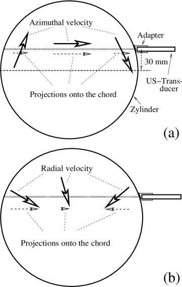
Figure 7: Sketch of the ultrasonic measurement set-up for the azimuthal velocity component. The obtained velocity along the chord is a position dependent mixture of radial and azimuthal components. In the middle of the chord, one gets the pure azimuthal component. (a) Typical situation for downward pumping with dominant azimuthal velocity (at the axial position 70 mm from the bottom). The projection of the velocity onto the chord has a maximum in the middle of the chord. (b) Typical situation for upward pumping with dominant radial velocity. The projection of the velocity goes to zero in the middle of the chord.

Two pairs of Helmholtz coils are fed by currents of 22.5 Ampere and 32.5 Ampere, respectively, to produce alternately an axial and a transversal field of 4 mT, which both are rather homogeneous throughout the vessel. Either field is applied for a period of 3 seconds, during which a trapezoidal signal form is used. The measurements are carried out for 0.5 seconds, 1 second after the plateau value of the trapezoidal current has been reached. Hence, we get an online monitoring with a time resolution of 6 seconds.

Figure 8: Measured projection of the velocity onto the chord, for downward and upward pumping. In the middle of the chord (at 85 mm distance from the wall) we get an azimuthal velocity of +0.58 m/s for downward pumping and -0.05 m/s for upward pumping (note the change of sign due to conventions in UDV measurements). Compare also Fig. 7 for illustration.

The induced magnetic fields are measured by 49 Hall sensors, 8 of them grouped together on each of 6 circuit boards which are located on different heights (Fig. 1). One additional sensor is located in the center below the vessel. The key problem of the method is the reliable determination of comparably small induced magnetic fields on the background of much higher imposed magnetic fields. An accurate control of the external magnetic field is essential to meet this goal. In our configuration the current drift in the Helmholtz coils can be controlled with an accuracy of better than 0.1 per cent. This is sufficient since the measured induced fields are approximately 1 per cent of the applied field. The temperature drift of the sensitivity can be overcome by enforcing the applied current in the Hall sensors to be constant. The temperature drift of the offset problem is circumvented by changing the sign of the applied magnetic field. Figure 2 shows that by these means a stable measurement of the small induced field can be realized, even over a period of one hour.

Figure 9: Azimuthal velocity at r=30 mm, as determined by CIFT at different axial positions. The small symbols (crosses and squares) represent individual measurements at six azimuthal positions. The large crosses and squares represent the corresponding averages over six azimuthal positions. The full symbols (circle and triangle) are the UDV values as inferred from Fig. 8.

For upward and downward pumping, Figs. 3 and 4 show the induced magnetic fields measured at the 49 positions, and the inferred velocity field at 52 discretization points. In Fig. 3c we see clearly the upward flow in the center of the vessel and the downward flow at the rim, but nearly no rotation of the flow in Fig. 3d. In Fig. 4c we can identify the downward flow in the center and the upward flow at the rim, and in Fig. 4d a clear rotation of the flow. Evidently, the method is able to identify the poloidal rolls and the absence or presence of the swirl.

For both flow directions, Fig. 5 illustrates the application of Tikhonov’s L-curves HANS . This curve, which results from scaling the parameter $\sigma_{pen}$ in Eq. (11) from lower to higher values, shows the dependence of the mean squared residual of the measured data on the kinetic energy of the flow. For low values (left end of Fig. 5) only little kinetic energy is allowed, leading to a velocity field that fits the measured magnetic field data only poorly. For high values (right end of Fig.5) the data are fitted very well but with an unphysical high kinetic energy. At the points of strongest bending (the ”knee”), the resulting velocities (Figs. 3 and 4) are physically most reasonable HANS .

IV Validation

In order to validate the CIFT method, we have performed independent velocity measurements based on ultrasonic Doppler velocimetry (UDV). For that purpose we have used the DOP2000 ultrasonic velocimeter manufactured by Signal-Processing SA (Lausanne, Switzerland), which had already demonstrated its capabilities for velocity measurements in liquid metals ECKE ; CRAMER . As ultrasonic transducers we have used 2 MHz probes.

Because of its comparably large magnetic Reynolds number ($Rm\approx 0.2$), the propeller driven flow in the cylinder has also a large hydrodynamic Reynolds number ($Re\approx 2\times 10^{5}$). Necessarily, the flow is highly turbulent. Strong fluctuations are observed both by the CIFT method as well as by UDV.

For a sensible comparison of both methods, some time averaging is advised. In the following we will focus on two UDV measurements that were both taken at a propeller rotation rate of 1200 rpm, and which represent a time average over half a minute.

The first measurement concerns the axial velocity along the central vertical axis of the cylinder. This axial component is easily measured by an ultrasonic transducer flash mounted to the bottom of the cylinder. Figure 6 shows the results of the UDV measurement (up to the propeller position), together with the results of the CIFT measurement. For both upward and downward pumping we see a reasonable correspondence of both measurements. Notably, CIFT exhibits the different axial dependencies that are typical for upward and downward pumping and which are confirmed by the UDV data.

The second measurement, which concerns the azimuthal velocity component, deserves some explanation. Figure 7 shows the UDV measurement set-up. The axial position is at 70 mm from the bottom. What is actually measured by UDV is the projection of the velocity onto the ultrasound beam along the chord. Therefore, the measured signal is in general a mixture of the radial and azimuthal velocity components. Only in the middle of the chord we get a signal that originates purely from the azimuthal velocity. In Figs. 7 (a) and (b) we illustrate the measured data that are shown in Fig. 8. In the case of downward pumping the velocity is dominated by the rotation whereas for upward pumping it is dominated by the radial part. In the middle of the chord we infer a mean azimuthal velocity of 0.58 m/s for downward pumping and -0.05 m/s for upward pumping.

Do these UDV values agree with those obtained by CIFT? In Fig. 9 we show the axial dependence of the azimuthal velocity at a radial position r=30 mm, as obtained by CIFT during a measurement time of 6 seconds. We give here the individual values at six different azimuthal positions (small crosses and squares). Interestingly, though the system is in general axisymmetric, non-axisymmetric fluctuations are still visible. The averages (large crosses and squares) over the six azimuthal positions show, at an axial position of z=70 mm, a good agreement with the data from UDV measurement.

V Conclusions and prospects

To summarize, we have put into practice a first version of contactless inductive flow tomography, using two orthogonal imposed magnetic fields. The comparison with UDV measurements shows that the method provides robust results on the main structure and the amplitude of the velocity field. A particular power of CIFT consists in a transient resolution of the full three-dimensional flow structure in steps of several seconds. Hence, slowly changing flow fields in various processes can be followed in time. Due to its weakness the externally applied magnetic field does not influence the flow to be measured. However, CIFT is also possible in cases where stronger magnetic fields are already present for the purpose of flow control, as, e.g., the electromagnetic brake in steel casting or the DC-field components in silicon crystal growth. Obviously, the future of the method lays with applying AC fields with different frequencies in order to improve the depth resolution of the velocity field. For problems with higher $Rm$, including dynamos, the inverse problem becomes non-linear, and more sophisticated inversion methods must be applied to infer the velocity structure from magnetic field data. Although interesting results have been obtained by employing Evolutionary Strategies to inverse spectral dynamo problems OSZI , and first tests of such inversion schemes for the data from the Riga dynamo experiment have shown promising results, the general inverse dynamo topic is extremely complicated and goes essentially beyond the scope of the present paper.

References

- (1) M. Hämäläinen, R. Hari, R. J. Ilmoniemi, J. Knuutila, and O. V. Lounasmaa, Rev. Mod. Phys. 65, 413 (1993).
- (2) A. Gailitis, O. Lielausis, E. Platacis, G. Gerbeth, and F. Stefani, Rev. Mod. Physics. 74, 973 (2002).
- (3) F. Stefani and G. Gerbeth, Inverse Probl. 15, 771 (1999).
- (4) J. A. Shercliff, The Theory of Electromagnetic Flow-Measurement, (Cambridge University, Cambridge, 1987).
- (5) M. Xu, F. Stefani, G. Gerbeth, J. Comp. Phys. 196, 102 (2004).
- (6) F. Pétrélis, M. Bourgoin, L. Marié, J. Burguete, A. Chiffaudel, F. Daviaud, S. Fauve, P. Odier, and J.-F. Pinton, Phys. Rev. Lett. 90, 174501 (2003).
- (7) F. Stefani and G. Gerbeth, Inverse Probl. 16, 1 (2000).
- (8) F. Stefani and G. Gerbeth, Meas. Sci. Technol. 11, 758 (2000).
- (9) P.C. Hansen, SIAM Review 34, 561 (1992).
- (10) S. Eckert and G. Gerbeth, Experiments in Fluids 32, 542 (2002).
- (11) A. Cramer, C. Zhang, S. Eckert, Flow Measurement and Instrumentation 15, 145 (2004).
- (12) F. Stefani and G. Gerbeth, Phys. Rev. E 67, 027302 (2003).