Discreteness-induced Stochastic Steady State in Reaction Diffusion Systems: Self-consistent Analysis and Stochastic Simulations
Abstract
A self-consistent equation to derive a discreteness-induced stochastic steady state is presented for reaction-diffusion systems. For this formalism, we use the so-called Kuramoto length, a typical distance over which a molecule diffuses in its lifetime, as was originally introduced to determine if local fluctuations influence globally the whole system. We show that this Kuramoto length is also relevant to determine whether the discreteness of molecules is significant or not. If the number of molecules of a certain species within the Kuramoto length is small and discrete, localization of some other chemicals is brought about, which can accelerate certain reactions. When this acceleration influences the concentration of the original molecule species, it is shown that a novel, stochastic steady state is induced that does not appear in the continuum limit. A theory to obtain and characterize this state is introduced, based on the self-consistent equation for chemical concentrations. This stochastic steady state is confirmed by numerical simulations on a certain reaction model, which agrees well with the theoretical estimation. Formation and coexistence of domains with different stochastic states are also reported, which is maintained by the discreteness. Relevance of our result to intracellular reactions is briefly discussed.
1 Introduction
Chemical reaction dynamics are often studied with the use of rate equations for chemical concentrations. For this approach, the number of molecules is assumed to be large, which validates the continuum description. However, in a biological system such as a cell, the number of molecules within is sometimes rather small. Then the validity of continuum description by the rate equations is not evident. This problem of smallness in molecule number is not restricted in biology. Following recent advances in nanotechnology, reactions in a micro-reactor are studied experimentally, where the number of molecules in concern is quite small. This is also true in some surface reaction of absorbed chemicals.
Here we are interested in the effect of such smallness in molecule number. Of course, one straightforward consequence of the smallness in the number is the large fluctuations in the concentration. Indeed, the fluctuations around the continuous rate equation can be discussed by stochastic differential equation [1, 2]. State change by noise has been studied as noise-induced transitions [3], noise-induced order [4], stochastic resonance [5], and so forth. The use of stochastic differential equation, as well as its consequence, has been investigated thoroughly. If the number of molecules is much smaller and can reach 0, however, another effect of ”smallness” is expected, that is the discreteness in the number. Our concern in the present paper is a drastic effect induced by such discreteness in the molecule number.
Previously we have discovered a transition of a chemical state, induced by the discreteness in the molecule number, i.e., the effect of the number of molecules , , [6]. The transition is termed as discreteness-induced transition (DIT). This transition is not explained by the stochastic differential equation approach. Rather, discreteness, in conjunction with the stochastic effect, is essential. In particular, we studied a system with autocatalytic reaction in a well stirred container. As the volume of the container decreases and the molecule number decreases, a transition to a novel state with symmetry breaking occurs, that does not appear either in the continuous rate equation or in its Langevin version. Here the transition occurs, when the number of molecule flow from environment to the reactor is discrete, in the sense that it is less than one on the average, within the average reaction time. Indeed, to the discreteness-induced transition, relevant is not the molecule number itself but the discreteness in the number of some molecular process (e.g., flow of molecule into the system) within the average time scale of some other reaction process.
On the other hand, in a spatially extended system with reaction and diffusion, the total number of molecules (and molecular events) increases with the system size, and is not small. Instead, the number of molecules (or events), not in the total system but within the size of an “effective length”, is relevant to determine the discreteness effect. Then, we need to answer what this effective length is. In [7], we have proposed that the so-called Kuramoto length gives an answer to it.
Kuramoto length is defined as the average length that a molecule diffuses within its lifetime, i.e., before it makes reaction with other molecules [1, 8, 9]. In the seminal papers [8, 9], Kuramoto has shown that whether the total system size is larger than this length or not provides a condition to guarantee the use of the reaction-diffusion equation. When the system size (length) is smaller than , local fluctuations rapidly spread over the system. Contrastingly, if the system size is much larger than , distant regions fluctuate independently, and the system is described by local reaction process and diffusion, validating the use of reaction-diffusion equation.
For example, consider the reaction
If the concentration of chemical is set to be constant, the chemical is produced at the constant rate , while it decays with the reaction at the rate . The average concentration of at the steady state is , where is the concentration of the chemical . Thus the average lifetime of at the steady state is estimated to be . If molecules diffuse at the diffusion constant in one-dimensional space, the typical length over which an molecule diffuses in its lifetime is estimated to be
| (1) |
which gives the Kuramoto length.
In these works, it is assumed that the average distance between molecules is much smaller than , and there is a large number of molecules within the region of the length . Thus the concentration of the chemical can be regarded as a continuous variable. Hence the continuum description is valid. However, if the average distance between molecules is comparable to or larger than , local discreteness of molecules may not be negligible.
For example, consider a chemical species , whose Kuramoto length is given by . Then we consider discreteness of molecule species that produces this chemical , i.e., the case that average number of is less than 1 within the area of the Kuramoto length . With this setting, molecules , produced by molecules, will be localized around them, as the average distance between molecules is larger than the Kuramoto length of . Then, this localization of the chemical may drastically alter the total rate of the reactions, if reactions with 2nd or higher order of are involved, as will be shown later. In the present paper, following [7], we pursue the possibility that discreteness of some molecules within Kuramoto length of some other molecules may drastically change the steady state of the system, as in DIT previously studied.
In section 2, we discuss a general condition for the amplification of some reaction by such discreteness. Then by introducing a self-consistent equation for the rate of this amplification, we demonstrate the existence of stable stochastic steady state (SSS), that never appears in the continuum description. In section 3, we numerically study a specific chemical reaction model with three components, to show the validity of this self-consistent theory for SSS. In section 4, domain formation with this SSS is presented, as a novel possibility for pattern formation in reaction-diffusion system. Discussion is given in section 5, with possible applications to biological problems.
2 Steady state induced by discreteness of molecule, with amplification of some reaction: self-consistent analysis
Consider a reaction system consisting of several molecule species (), with chemical reaction and diffusion. The system can involve catalytic reactions of higher-order catalysis or autocatalysis. Some other molecules (e.g., resource chemicals) are supplied externally, involved in the reaction among , so that the nonequilibrium condition is sustained. So far the system in concern is rather general chemical reaction system with diffusion.
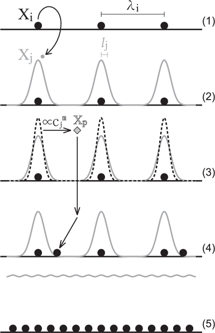
Now, we take a pair of molecule species, and , where is produced by , and study how the discreteness of the molecule can alter the steady state from the continuum limit case. To discuss the discreteness effect, we consider the case that the molecule is localized around the molecule . (Recall the molecule is produced by .) In order for this localization to work, the average length that the molecule travels within its lifetime should be smaller than the average distance of the molecules . In other words, the average number of the molecules within the domain of the Kuramoto length is less than 1. (see Fig. 1). Here, the lifetime of the molecule is determined by the collision with some other molecule species whose density is not low. Hence, the Kuramoto length of the molecule, determined as in §1, is given independently of the concentrations of the molecules and .
Now, to alter drastically the steady state by discreteness, the localization of molecule has to change concentrations of some other molecules, as compared with the case of homogeneous distribution of . This is possible if there is a higher-order reaction such as , because the probability of such reaction is amplified by localization of molecules in space. To compute this acceleration, we calculate the average of , where is the concentration of , and compute the degree of amplification from that for the homogeneously distributed case. In the calculation, we assume that is localized around the molecules, with a width of , the Kuramoto Length of (which is shorter than the average distance between molecules).
Assuming that the distribution of is represented by the continuous concentration , can be expressed as
| (2) |
where is the size (volume) of the system.
For simplicity, we assume that is randomly distributed over -dimensional space, and the distribution of is given by a -dimensional Gaussian distribution with a standard deviation around each molecule, such as
where is the position of each molecule. Now is the sum of ; thus, since . For the case with and sufficiently large ,
since is randomly distributed. With eq. (2),
Thus, we obtain the acceleration factor
| (3) |
In the same manner, for ,
| (4) |
and generally, for ,
| (5) |
As shown, the reaction can be drastically amplified as the number of molecules within a volume of the Kuramoto length () is much smaller than 1.
So far we have shown that for reaction system involving the process from to , the discreteness can alter the concentration of some chemicals drastically, if (1) the density of molecule is so low that the number is discrete within the size of the Kuramoto length of molecule and (2) there is a high order (higher than linear) reaction with regards to .
Next, to confirm that this acceleration of reaction alters the steady state from the continuum case, we need to check if the condition for the discreteness is sustained under the above amplification of concentration of some chemicals, as a steady state solution. Hence we study some feedback from the concentration of to that is generated by some reaction path(s). If is produced or catalyzed by , the concentration of depends on that of , . With such feedback, the change of concentration is given by some function , while the change of the concentration depends on , and is given by some function as . Since is a function of , is rewritten as . Hence the concentrations of and molecules must satisfy
| (6) |
( and may have dependence on other concentrations or reaction rates, e.g., can also depend on or ). The steady state solution is obtained by setting the right hand of these equations as 0.
Note that the solution with corresponds to the continuum case, given by the standard rate equation. For some case, this is the only solution for the concentrations. For some other cases, however, there is some other solution(s) with . This is a solution with the amplification by localization of molecules due to the discreteness of the molecule. If the concentration of obtained from this solution satisfies , this discreteness-induced solution is self-consistent. Furthermore, the stability of this solution is computed by linearizing the solution around this fixed point. If this solution is linearly stable, stability of this novel steady solution is assured, which does not exist in the continuum description (or in its Langevin equation version). We call the state represented by this solution as stochastic steady state (SSS), as it is sustained stochastically through discreteness in molecule numbers. We will show an explicit example of this SSS in the next section.
Self-consistent solution involving the change of Kuramoto-length
So far we have assumed that the Kuramoto-length of the molecule is constant. This is true as long as the concentration of the molecule relevant to the decomposition or transformation of the molecule is constant. However, if the concentration of the chemical that is relevant to the determination of depends on the concentration of either , , or , the Kuramoto length, as well as , depends on it. Accordingly, in eq. (6), we need to regard in as a variable that depends on either , or . With the inclusion of the dependence, we again obtain a self-consistent solution, to get the concentrations and (and accordingly and ). If there is a stable solution with and , then we get a SSS as a self-consistent solution both on and . We will discuss a related example in §4, where two solutions with and coexist in space, and form a domain structure.
Combination of several processes
So far we have discussed a simple case of discreteness-induced state. The discussion with the use of amplification factor , however, is generalized to include temporally or spatially dependent solutions of and , with temporal (or spatial) dependence of . This solution represents an average behavior longer than the time scale for stochastic collisions or longer scale than . With this extension, we can discuss discreteness-induced rhythm or pattern, that is stochastically sustained.
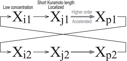
Such spatiotemporal dynamics can often appear in a reaction network of several molecules, with two or more pairs of discreteness in number. For example, consider reactions , , ; and , , (see Fig. 2), where we assume that the density , , of and molecules are so low that and , respectively for the Kuramoto lengths of and . Then, following the scheme we discussed, we get a coupled equation for the concentrations of , , , with two amplification factors and . In general, there may be a time- or space- dependent solution (by including diffusion term with much longer spatial scale), that leads to a novel stochastic pattern or rhythm. Explicit examples for such case will be discussed in future.
3 Specific example of Stochastic Steady State
To confirm our theoretical estimation for SSS, we have adopted a simple model and carried out stochastic particle simulations. Here we consider a simple one-dimensional reaction-diffusion system with three chemicals (, , and ) and four reactions:
Here, we assume . We take , , and (, ) for further discussion. We assume that the system is closed with regards to the molecules . Thus, , the total number of molecules (or , the total concentration), is conserved.
In the continuum limit, each , the concentration of at time and position , obeys the following reaction-diffusion equation:
| (7) | |||||
| (8) | |||||
| (9) |
where is the diffusion constant of . For simplicity, we assume for all . This reaction-diffusion equation has homogeneous fixed point solutions with , for all . By linear stability analysis, it is straightforward to show that only the former is stable. Starting from any initial conditions, the partial-differential equation system simply converges to this stable fixed point.
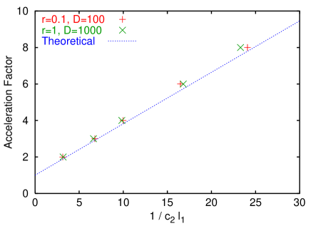
In this system, the chemical is produced by molecules. (In the notation of §2, and .) If , the Kuramoto length of , is shorter than the average distance between molecules, is localized around the molecules, as discussed in §2. Then, the reaction , which is at second order of , is accelerated. Using eq. (3) in §2, we obtain the acceleration factor
| (10) |
On the other hand, the lifetime of is so long that is not localized. Thus, the reaction is not accelerated.
Now we study the self-consistent solution from and , following the argument of §2. (By a path from to , there is a direct feedback to , i.e., in the notation of §2.) Here, we consider the case where , , so that . Then, the average lifetime of is about ; we assume that for further discussion. When , , the two reactions and are much faster than the other two and maintain . Then, the rates of the other reactions satisfy
| (11) |
When , the two reactions are balanced, which leads to a novel fixed point. Assuming and , and following eq. (10), we obtain the condition for the balance
| (12) |
Subsequently, we investigate the stability of this fixed point. For and , we obtain
| (13) |
from eqs. (10) and (12). We take into account the acceleration factor in the reaction-diffusion equation, we obtain
| (21) | |||||
For any , , this Jacobi matrix has two negative eigenvalues, implying that the fixed point is stable111It is also stable against spatially inhomogeneous perturbations for any ..
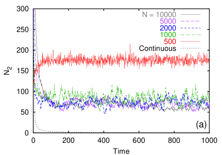
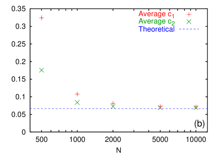
In the simulations, we have found that the system converges to the novel fixed point. In fact, we have measured at the fixed point for a certain numerically. Figure 4 shows the relation between and , which agrees rather well with the theoretical estimation in eq. (10).
In summary, we demonstrated numerically that the discreteness of molecules yields a novel stochastic steady state in a reaction-diffusion system, in agreement with the theoretical estimation.
4 Coexistence of Domains with different Kuramoto Lengths
In the example of the previous section, the spatial homogeneity is assumed at a coarse-grained level, and indeed, this homogeneous state was stable. However, due to fluctuations, some spatial inhomogeneity exists in SSS, and a domain that is deviated from SSS may be produced. Even if this deviated state is unstable in the continuum limit, it may be preserved over a long time, if the concentration of the molecule to destabilize it is so low that its discreteness is essential. If the average time to produce this deviated domain from SSS and the lifetime of the state is balanced, the two regions, SSS and the deviated state with different concentrations of molecules and Kuramoto lengths, may coexist. We give a simple example for it here.
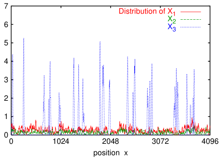
Again we consider the same reactions as the preceding section. Now, we assume that the diffusion of is slower than the others, and set (). In this model, there are two fixed-point states: one is the stochastic steady state mentioned above (which we call State A); the other is the unstable fixed point with (State B), besides the stable fixed point in the continuum limit (which does not appear here; see Table 1 for the stability of the states mentioned here). In Fig. 5, we give an example of snapshot pattern of the model. In the figure, except several spots with large that corresponds to the state A, most other regions fall onto the state B that should be unstable in the continuum limit. Indeed, this pattern is not transient, and the fraction of the state B is stationary, in the long-term simulation. This suggests the possibility that the state B, unstable in the continuum limit, may be sustained over a finite period due to the discreteness in molecules, which forms a domain in space. The two states A and B coexist in space and form a domain structure.
| state | continuous | discrete | |
|---|---|---|---|
| the unstable fixed point of the R-D eq. | unstable | unstable | |
| the stochastic steady state | (not fixed point) | stable | |
| the stable fixed point of the R-D eq. | stable | unstable |
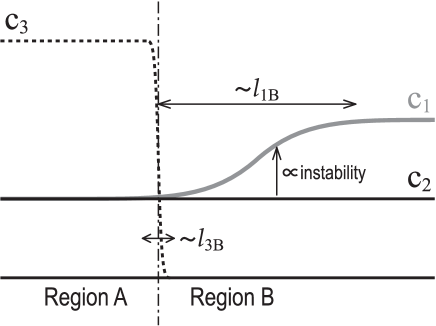
First, we consider stability of each of the states in more detail. The state B is unstable against the inflow of . If an molecule enters into a region of state B (Region B), it can be amplified and form a new region (spot) of the state A (Region A). From linear stability analysis, we find that the degree of instability of the region B against the flow of is proportional to . Note that in the region A, , while in the region B, , and . Here, the concentration is almost uniform in space because of its long lifetime. Thus, the degree of the instability of the Region A, that is the rate of growth of , depends mainly on the distribution of (see Fig. 6).
Accordingly, the Kuramoto length of is relevant to determine if the state B is invaded or not. Here it should be noted that in the region A, is smaller than that in the region B. Hence in the vicinity of the region A within the domain of the state B, is still small, as long as it is within the Kuramoto length of of the region A. Thus the instability is weak there, which prevents a novel region A ( spot) growing in the vicinity of the existing region A. Hence, the interval between two neighboring regions A should be longer than the Kuramoto length of . Assuming that , and (i.e., the unstable fixed point of the reaction-diffusion equation) in the region B, we obtain the Kuramoto length of in the region B as
Since can be amplified by using in the region B, penetration of molecules into the region B must be rare in order to maintain the region B. The penetration length is given by the Kuramoto length of , that is computed as
for the region B. For , , which implies that molecules seldom reach the area where is strongly amplified. Thus, the border of regions A and B is maintained for long time222For this reason, we set relatively small. If is larger, the border is blurred and the two regions are mixed..
On the other hand, due to the fluctuation inherent in SSS, the molecule may be extinct within some area of the region A, with some probability. Hence, the regions A and B coexist in space, as shown in Fig. 5. As shown, the region A is localized only as spots, and other parts are covered by the region B.
Note that in the corresponding reaction-diffusion equations, the state A, the stochastic steady state, cannot be realized, while the state B is unstable. Indeed, the reaction-diffusion equation system is quickly homogenized and converges to the stable fixed point with . Hence both the regions A and B, as well as a domain structure from the two, can exist only as a result of the discreteness of molecules, and are immediately destroyed in the continuum limit.
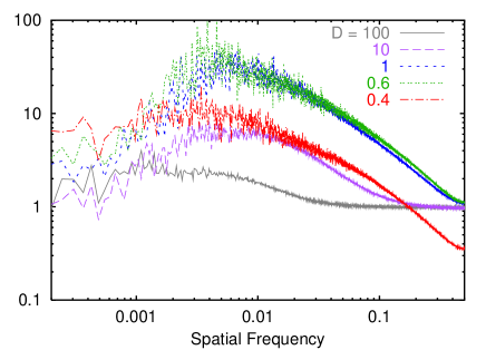
Note that in the present model, SSS does not have so-called the Turing instability333It is also possible that the acceleration of reactions by the discreteness induces or enhances the Turing instability in certain systems., and there is no characteristic wavelength. Still the spatial structure here has some characteristic length, as given by the minimal size of the region B, estimated by the Kuramoto length . In Fig. 7, we have plotted the spatial power spectrum of the concentrations of . Although there is no clear peak, there is a very broad increase around the wavenumber of , that corresponds to average domain size of the region B.
In general, the discreteness of molecules can induce novel states not seen in the continuum limit. For example, in a randomly connected catalytic reaction network, there often exist several fixed points with some chemicals going extinct, when the number of molecules is small, while there is only one attractor in the continuum limit. These discreteness-induced states may coexist in space in a similar way as discussed above. Kuramoto length will be a useful index to determine the behavior around the border of the regions.
5 Summary and Discussion
In the present paper, we have reported a novel steady state in a system with reaction and diffusion, induced by discreteness in molecules. This state cannot be represented by a continuum description, i.e., partial differential equation (reaction-diffusion equation), but is sustained by amplification of some reaction due to localization of some molecule . This localization is possible if the molecule species that produce is “discrete”, in the sense that its average number within the Kuramoto length of the molecule is less than 1. We have formulated a theory to obtain a self-consistent solution for the concentrations of and , in relationship with the amplification rate of the reaction involved with . For some reaction system, there is a solution with amplification rate larger than 1, that leads to the existence of stochastic steady state due to the discreteness in molecule number. The stability of this solution is also computed within this theoretical formulation.
We have also numerically studied a simple reaction-diffusion system to demonstrate the validity of the theory. Indeed, a novel stochastic steady state is observed, as predicted theoretically. We have also extended our theory to include the self-consistent determination of the Kuramoto length. Following this extension, we have provided a numerical example, to show formation of domains with different Kuramoto lengths.
The alteration of the steady state by the localization, as well as our formulation for it is quite general. Provided that the conditions
-
(i)
Chemical generates another chemical species .
-
(ii)
The lifetime of is short or the diffusion of is slow so that the Kuramoto length of is much smaller than the distance between molecules.
-
(iii)
The localization of the molecule accelerates some reactions.
Then, the discreteness can alter the dynamics, from that by the continuum description. The last condition is satisfied if the second or higher order reaction is involved in the species . Finally, if
-
(iv)
the acceleration of the reaction in (iii) alters the density of molecules, through some reaction(s),
the density of is determined self-consistently with the acceleration factor, resulting in a novel steady state.
Note that the localization effect by the discreteness of catalytic molecules itself is also noted by Shnerb et al. [10]. In their study, however, the density of the catalyst is fixed as an externally given value. Thus the concentration of the product, localized around the catalyst, diverges in time. In our theory, the density of the catalyst () changes autonomously and reaches a suitable value by following the discreteness effect.
The self-consistent solution scheme to obtain this discreteness-induced stochastic state can be extended to a case with several components , and the corresponding set of chemicals satisfying the conditions (i)–(iii). In such case, the feedback process in (iv) is not necessarily direct from to . If there is a feedback from the set of chemicals to the set (condition (iv)′), the above scheme for the self-consistent dynamics we presented here works. With this extension, there is a variety of possibilities, that can lead to stochastic rhythm or pattern formation induced by discreteness of molecules, which is not seen in the continuum limit. For example, in a catalytic reaction network with many components and a limited number of total molecules, there always exist several species that are minority in number, and the conditions (i)–(ii) are naturally satisfied, while with higher order catalytic reaction the condition (iii) is often satisfied. In this case, minority molecules become a key factor to determine a macroscopic state with rhythm or pattern. (Note in this case, other molecules can be abundant in number, or indeed it is better to have such abundant species, so that the stochastic state is stabilized.)
In fact, biochemical reaction networks involve a huge number of species, while the total number of molecules is not necessarily so large. In a cell, lots of chemicals work at low concentration in the order of 1 nM or less. The diffusion is sometimes restricted, surrounded by macro-molecules, and may be slow. In such an environment, it is probable that the average distance between the molecules of a given chemical species is much larger than the Kuramoto lengths of some other chemical species. Some chemicals are localized around some other molecules. Furthermore, biochemical systems contain various higher order reactions (for example, catalyzed by enzyme complexes). In conjunction with the localization, such reactions can be accelerated. Hence the conditions (i)–(iii) are ubiquitously satisfied in intra-cellular biochemical reaction networks. In addition, since the biochemical reactions involve complex feedback process through mutual catalytic networks, the condition (iv) or (iv)′ is naturally satisfied.
Accordingly, it will be important to study the amplification of some reaction and its maintenance through feedback will be relevant to biochemical reactions. Indeed, some molecules that are minority in number sometimes play a key role in biological function. Relevance of minority molecules is also discussed from the viewpoint on a control mechanism of a cell, in relationship with the kinetic origin of information [11, 12].
The importance of our theory is not restricted to biological problems. Verification of our result will be possible by suitably designing a reaction system, with the use of, say, microreactors or vesicles. The acceleration and maintenance of some reactions by localization of molecules will be important to design some function in such micro-reactor systems.
Acknowledgement
The present paper is dedicated to Professor Yoshiki Kuramoto on the occasion of his retirement from Kyoto University. With the papers [8, 9] that introduced Kuramoto length a novel research field was opened; the study of chemical wave and turbulence with the use of continuous, deterministic reaction-diffusion equation. It is our pleasure to use his length in the opposite context here, for the description of novel steady states in discrete, stochastic reaction-diffusion systems. The present work is supported by grant-in-aid for scientific research from the Ministry of Education, Culture, Sports, Science and Technology of Japan (15-11161), and the Japan Society for the Promotion of Science.
References
- [1] N. G. van Kampen, Stochastic processes in physics and chemistry (North-Holland, rev. ed., 1992).
- [2] R. Kubo, K. Matsuo, and K. Kitahara, “Fluctuation and Relaxation of Macrovariables”, Jour. Stat. Phys. 9, 51 (1973).
- [3] W. Horsthemke and R. Lefever, Noise-Induced Transitions, edited by H. Haken (Springer, 1984).
- [4] K. Matsumoto and I. Tsuda, “Noise-Induced Order”, Jour. Stat. Phys. 31, 87 (1983).
- [5] R. Benzi, G. Parisi, A. Sutera and A. Vulpiani, “Stochastic resonance in climatic change”, Tellus 34, 10 (1982).
- [6] Y. Togashi and K. Kaneko, “Transitions induced by the discreteness of molecules in a small autocatalytic system”, Phys. Rev. Lett. 86, 2459 (2001).
- [7] Y. Togashi and K. Kaneko, “Molecular discreteness in reaction-diffusion systems yields steady states not seen in the continuum limit”, to appear in Phys. Rev. E (2004).
- [8] Y. Kuramoto, “Fluctuations around Steady States in Chemical Kinetics”, Prog. Theor. Phys. 49, 1782 (1973).
- [9] Y. Kuramoto, “Effects of Diffusion on the Fluctuations in Open Chemical Systems”, Prog. Theor. Phys. 52, 711 (1974).
- [10] N. M. Shnerb, Y. Louzoun, E. Bettelheim, and S. Solomon, “The importance of being discrete: Life always wins on the surface”, Proc. Nat. Acad. Sci. 97, 10322 (2000).
- [11] K. Kaneko and T. Yomo, “On a Kinetic Origin of Heredity: Minority Control in a Replicating System with Mutually Catalytic Molecules”, Jour. Theor. Biol. 214, 563 (2002).
- [12] K. Kaneko, “Recursiveness, switching, and fluctuations in a replicating catalytic network”, Phys. Rev. E 68, 031909 (2003).