Novel Gravity Probe B Gravitational Wave Detection

Abstract

The Gravity Probe B (GP-B) satellite experiment will measure the precession of on-board gyroscopes to extraordinary accuracy. Such precessions are predicted by General Relativity (GR), and one component of this precession is the ‘frame-dragging’ or Lense-Thirring effect, which is caused by the rotation of the earth, and the other is the geodetic effect. A new theory of gravity predicts, however, a second and much larger ‘frame-dragging’ or vorticity induced spin precession. This spin precession component will also display the effects of novel gravitational waves which are predicted by the new theory of gravity, and which have already been seen in several experiments. The magnitude and signature of these gravitational wave induced spin precession effects is given for comparison with the GP-B experimental data.

1 Introduction

The Stanford University-NASA Gravity Probe B satellite experiment has the capacity to measure the precession of four on-board gyroscopes to unprecedented accuracy [1, 2, 3, 4, 5]. The experiment was proposed independently by George Pugh in 1959 and Leonard Schiff in 1960. Such a precession is predicted by the Einstein theory of gravity, General Relativity (GR), with two components: (i) a geodetic precession, and (ii) a ‘frame-dragging’ precession known as the Lense-Thirring effect. The latter is a particularly interesting effect induced by the rotation of the earth, and described in GR in terms of a ‘gravitomagnetic’ field. According to GR this smaller effect will give a precession perpendicular to the plane of the satellite orbit accumulating to 0.042 arcsec per year for the GP-B gyroscopes. However a recently developed theory gives a different account of gravity [6, 11]. This theory gives a dynamical account of the so-called ‘dark matter’ effect in spiral galaxies. It also successfully predicts the masses of the black holes found in the globular clusters M15 and G1. Here we show that GR and the new theory make very different predictions for the ‘frame-dragging’ effect, and so the GP-B experiment will be able to decisively test both theories. While predicting the same earth-rotation induced precession, the new theory has an additional much larger ‘frame-dragging’ effect caused by the observed translational motion of the earth, and in a different direction to the earth induced rotation induced precession. As well the new non-metric theory explains the ‘frame-dragging’ effect in terms of vorticity in a ‘substratum flow’. This ‘flow’ exhibits fluctuations or wave effects that have already been seen in at least three experiments. These are the gravitational waves of the new theory of gravity, and are completely different from the gravitational waves predicted by General Relativity. Herein the magnitude and signature of this new component of the gyroscope precession is predicted, with particular emphasis on the gravitational wave effects, which it is predicted will be detectable by the GP-B experiment.

2 Aspects of the History of Gravity Research

The history of the development of theories of gravity is well known. Newton introduced the gravitational acceleration field ${\bf g}({\bf r},t)$, whose source was matter, as shown in (2), and which was then used by Newton to explain the solar system planetary dynamics as had been expressed by Kepler in his laws. In terms of this acceleration field Newton’s ‘universal law of gravitation’, in (1), is uniquely determined by Kepler’s laws. However the phenomena of gravity may be equally well represented in terms of a ‘flow’ system involving a velocity vector field ${\bf v}({\bf r},t)$, and this formalism is physically indistinguishable from the Newtonian formalism, in terms of the consequent gravitational forces in the solar system, though it is clearly different mathematically. However, unlike the Newtonian formalism, this velocity field formalism permits an additional dynamical effect that would not have manifested in the case of the solar system, that is, it is not inconsistent with Kepler’s laws. It is now known that this additional dynamical effect is nothing more than the so-called ‘dark matter’ effect [6]. So we now understand that had Newton used the velocity field instead of the acceleration field as the fundamental degrees of freedom then the ‘dark matter’ effect could have been predicted by Newton long ago.

There was another ‘accident of history’ that has enormously influenced the development of physics, and in particular that of gravity, namely the detection of absolute motion. In this case Michelson and Morley in their interferometer experiment of 1887 detected the expected fringe shifts caused by absolute motion, but using Newtonian physics Michelson had developed a theory for the instrument which predicted fringe shifts larger than actually observed. This supposed failure to detect the expected fringe shifts and so absolute motion led to the notion that absolute motion, that is, motion measured with respect to local space itself, is not even a meaningful concept, despite that over the last 114 years it has been detected in at least seven experiments, and of several kinds. Re-analysing the operation of the Michelson interferometer by taking account, for the first time, of both the Fitzgerald-Lorentz contraction effect and the effect of a gas being present in the light path, we now know that the Michelson-Morley experiment gives a lower limit of some 300 km/s for the speed of absolute motion of the earth through space, rather than the 8 km/s which follows from the Newtonian theory and which they reported in 1887. The existence of absolute motion and of the gravitational effects associated with that ‘flow’ have gone unstudied for the last 100 years, and the ‘dark-matter’ effect is only one of numerous gravitational phenomena that have been observed but remain as unexplained - these phenomena are known as ‘gravitational anomalies’. It always needs to be emphasised that absolute motion is the cause of the various relativistic effects, an idea that goes back to Lorentz in the 19^th century.

In 1916 Hilbert and Einstein proposed a metric spacetime theory of gravity, which was constructed to agree with the Newtonian acceleration field formalism in the so-called non-relativistic limit. But in doing so Hilbert and Einstein consequently missed the ‘dark matter’ effect, as that effect had been missed also by Newton. As well this theory also missed the existence of absolute motion, an effect absolutely critical to understanding gravity. It has been repeatedly claimed that the Hilbert-Einstein General Theory of Relativity has been confirmed many times, but this is untrue. All but one of the so-called tests merely used the geodesic equation which determines the trajectory of a particle or an electromagnetic wave in a given metric. That metric has in all cases been the external Schwarzschild metric, but apparently unknown to most is that this metric is nothing more than the Newtonian ‘inverse square law’ in mathematical disguise, namely with the metric expressed in terms of the particular velocity vector flow field corresponding to Newton’s inverse square law. So these tests of GR were confirming, at best, the flow formalism for gravity, together with its geodesic equation, and had nothing to do with the dynamical content of GR. Indeed the one single test, so far, of GR is the observed decay rate of the binary pulsar orbits. As well, as already noted, GR has failed in the case of the ‘dark matter’ effect.

The Gravity Probe B experiment will test the dynamics of GR and of the new theory, and the differences between the two predictions are very different. Because of the denial of absolute linear motion in GR it predicts only a ‘frame-dragging’ effect produced by the absolute rotation of the earth, whereas the new theory of gravity predicts not only that effect, but most significantly and dominantly, a ‘frame-dragging’ effect caused by the absolute linear motion of the earth. In the new theory, because it is not a metric spacetime theory, the ‘spacetime frame-dragging’ is seen to be a vorticity in the flow of space caused by the absolute motion of the earth, both rotational and linear, through that space. As well that flow has wave phenomena which can be detected via their effect on the vorticity. The vorticity of the flow, which is simply a local rotation of the direction of the flow, affects the GP-B gyroscopes, and anything else, by simply rotating the whole system. So the gyroscope spin precessions can detect these gravitational waves.

As well the ‘dark matter’ dynamical effect has its magnitude determined by a new dimensionless gravitational constant, in addition to the Newtonian constant $G$. By comparing the new theory with the experimental data from the Greenland borehole $g$ anomaly data, it was found that the new gravitational constant is the fine structure constant $\alpha\approx 1/137$. This has enormous implications for fundamental physics, as discussed elsewhere [6], but in particular the new theory predicts black holes whose dynamics is determined by the value of $\alpha$, and not by $G$. This result has been confirmed by the black holes observed in several globular clusters. The ‘dark matter’ effect is also apparent in Cavendish-type experiments that measure $G$, and there has been a longstanding unknown systematic effect present in these experiments that has caused $G$ to be the least accurately known fundamental constant [6].

3 A Theory of Gravity

Here we briefly review the derivation of the new theory of gravity [6, 11]. The Newtonian ‘inverse square law’ for gravity,

$$F=\frac{Gm_{1}m_{2}}{r^{2}},$$ (1)

was based on Kepler’s laws for the motion of the planets. Newton’s ‘explanation’ of the phenomena of gravity was in terms of the gravitational acceleration vector field ${\bf g}({\bf r},t)$, and in differential form

$$\nabla.{\bf g}=-4\pi G\rho,$$ (2)

where $\rho({\bf r},t)$ is the matter density. However there is an alternative formulation [6] in terms of a vector ‘flow’ field ${\bf v}({\bf r},t)$ determined by

$$\frac{\partial}{\partial t}(\nabla.{\bf v})+\nabla.(({\bf v}.{\bf\nabla}){\bf v})=-4\pi G\rho,$$ (3)

with ${\bf g}$ now given by the Euler ‘fluid’ acceleration

$${\bf g}=\displaystyle{\frac{\partial{\bf v}}{\partial t}}+({\bf v}.{\bf\nabla}){\bf v}=\displaystyle{\frac{d{\bf v}}{dt}}.$$ (4)

Trivially this ${\bf g}$ also satisfies (2). External to a spherical mass $M$ of radius $R$ a velocity field solution of (3) is

$${\bf v}({\bf r})=-\sqrt{\frac{2GM}{r}}\hat{\bf r},\mbox{\ \ }r>R,$$ (5)

which gives from (4) the usual inverse square law ${\bf g}$ field

$${\bf g}({\bf r})=-\frac{GM}{r^{2}}\hat{\bf r},\mbox{\ \ }r>R.$$ (6)

However the flow equation (3) is not uniquely determined by Kepler’s laws because

$$\frac{\partial}{\partial t}(\nabla.{\bf v})+\nabla.(({\bf v}.{\bf\nabla}){\bf v})+C({\bf v})=-4\pi G\rho,$$ (7)

where

$$C({\bf v})=\displaystyle{\frac{\alpha}{8}}((trD)^{2}-tr(D^{2})),$$ (8)

and

$$D_{ij}=\frac{1}{2}\left(\frac{\partial v_{i}}{\partial x_{j}}+\frac{\partial v_{j}}{\partial x_{i}}\right),$$ (9)

also has the same external solution (5), because $C({\bf v})=0$ for the flow in (5). So the presence of the $C({\bf v})$ would not have manifested in the special case of planets in orbit about the massive central sun. Here $\alpha$ is a dimensionless constant - a new gravitational constant, in addition to usual the Newtonian gravitational constant $G$. However inside a spherical mass we find [6] that $C({\bf v})\neq 0$, and using the Greenland borehole $g$ anomaly data [8] we find that $\alpha^{-1}=139\pm 5$, which gives the fine structure constant $\alpha=e^{2}\hbar/c\approx 1/137$ to within experimental error. From (4) we can write

$$\nabla.{\bf g}=-4\pi G\rho-4\pi G\rho_{DM},$$ (10)

where

$$\rho_{DM}({\bf r})=\frac{\alpha}{32\pi G}((trD)^{2}-tr(D^{2})),$$ (11)

which introduces an effective ‘matter density’ representing the flow dynamics associated with the $C({\bf v})$ term. In [6] this dynamical effect is shown to be the ‘dark matter’ effect. The interpretation of the vector flow field ${\bf v}$ is that it is a manifestation, at the classical level, of a quantum substratum to space; the flow is a rearrangement of that substratum, and not a flow through space. However (7) needs to be further generalised [6] to include vorticity, and also the effect of the motion of matter through this substratum via

$${\bf v}_{R}({\bf r}_{0}(t),t)={\bf v}_{0}(t)-{\bf v}({\bf r}_{0}(t),t),$$ (12)

where ${\bf v}_{0}(t)$ is the velocity of an object, at ${\bf r}_{0}(t)$, relative to the same frame of reference that defines the flow field; then ${\bf v}_{R}$ is the velocity of that matter relative to the substratum. The flow equation (7) is then generalised to, with $d/dt=\partial/\partial t+{\bf v}.\nabla$ the Euler fluid or total derivative,

$$\frac{dD_{ij}}{dt}+\frac{\delta_{ij}}{3}tr(D^{2})+\frac{trD}{2}(D_{ij}-\frac{\delta_{ij}}{3}trD)+\frac{\delta_{ij}}{3}\frac{\alpha}{8}((trD)^{2}-tr(D^{2}))$$

$$+(\Omega D-D\Omega)_{ij}=-4\pi G\rho(\frac{\delta_{ij}}{3}+\frac{v^{i}_{R}v^{j}_{R}}{2c^{2}}+..),\mbox{ }i,j=1,2,3.$$ (13)

$$\nabla\times(\nabla\times{\bf v})=\frac{8\pi G\rho}{c^{2}}{\bf v}_{R},$$ (14)

$$\Omega_{ij}=\frac{1}{2}\left(\frac{\partial v_{i}}{\partial x_{j}}-\frac{\partial v_{j}}{\partial x_{i}}\right)=-\frac{1}{2}\epsilon_{ijk}\omega_{k}=-\frac{1}{2}\epsilon_{ijk}(\nabla\times{\bf v})_{k},$$ (15)

and the vorticity vector field is $\vec{\omega}=\nabla\times{\bf v}$. For zero vorticity and $v_{R}\ll c$ (13) reduces to (7). We obtain from (14) the Biot-Savart form for the vorticity

$$\vec{\omega}({\bf r},t)=\frac{2G}{c^{2}}\int d^{3}r^{\prime}\frac{\rho({\bf r}^{\prime},t)}{|{\bf r}-{\bf r}^{\prime}|^{3}}{\bf v}_{R}({\bf r}^{\prime},t)\times({\bf r}-{\bf r}^{\prime}).$$ (16)

The GP-B experiment will detect this vorticity field by means of the spin-axis rotation or precession of the gyroscopes over time, with the magnitude and direction of this rotation or precession measured relative to the direction of the guide star as observed by the on-board telescope. Clearly any wave phenomena that changes ${\bf v}_{R}({\bf r},t)$ in (16) will also be detected via its effect on $\vec{\omega}({\bf r},t)$.

4 Geodesics

We now define how the trajectory of a point object is determined by the velocity flow field, which manifests via the velocity of absolute motion of the object relative to the local space, namely via ${\bf v}_{R}$. There is a problem with terminology here: what is called absolute motion here is actually motion with respect to the local substratum structure of space, which means that it is a relative motion. However in the language and restrictions of conventional ‘special relativity’ all velocities are relative, where in this case it means relative to another object and not relative to space itself. Most significantly the geodesic equation herein involves both (absolute) motion with respect to space and also the relativistic time dilation effect. This latter effect involves the notion that absolute motion, whether linear or rotational, causes, say, a clock moving through space to tick more slowly than one at rest in space. Similarly in the re-analysis of the principles of operation of the Michelson interferometer it was necessary to take account of both absolute linear motion and the relativistic length contraction effect upon the arms of the interferometer caused by that absolute linear motion. So again to observe absolute motion we must take account of those relativistic effects which are actually caused by absolute motion. This is contrary to the postulate by Einstein which asserts that absolute motion has no meaning and so no experimental manifestation. The GP-B experiment will, yet again, show that this key postulate is invalid, but which does not invalidate the phenomena known as ‘special relativistic’ effects. In terms of the history of physics it implies that we must return to the pre-Einstein ideas of Lorentz and others.

The path ${\bf r}_{0}(t)$ of an object through space is obtained by extremising the relativistic proper time

$$\tau[{\bf r}_{0}]=\int dt\left(1-\frac{{\bf v}_{R}^{2}}{c^{2}}\right)^{1/2}$$ (17)

This entails the idea that the speed of light $c$ is the maximum speed through the local space. This means that the speed of light is $c$ only with respect to the local space. That it is believed that $c$ is the speed of light for all observers in uniform linear motion, as postulated by Einstein, is an error that follows from not realising that when in motion the observer’s clock and rod are affected by that motion. Without correcting for such absolute motion effects the incorrect notion of $c$ being the ‘universal speed of light’ is not realised.

To extremise $\tau$ we use a small deformation of the trajectory

$${\bf r}_{0}(t)\rightarrow{\bf r}_{0}(t)+\delta{\bf r}_{0}(t)\mbox{\ \ giving \ \ }{\bf v}_{0}(t)\rightarrow{\bf v}_{0}(t)+\displaystyle\frac{d\delta{\bf r}_{0}(t)}{dt},$$ (18)

and then we also have

$${\bf v}({\bf r}_{0}(t)+\delta{\bf r}_{0}(t),t)={\bf v}({\bf r}_{0}(t),t)+(\delta{\bf r}_{0}(t).{\bf\nabla}){\bf v}({\bf r}_{0}(t))+...$$ (19)

Then

$$\delta\tau = \tau[{\bf r}_{0}+\delta{\bf r}_{0}]-\tau[{\bf r}_{0}]$$

$$= -\int dt\>\frac{1}{c^{2}}{\bf v}_{{R}}.\delta{\bf v}_{{R}}\left(1-\displaystyle{\frac{{\bf v}_{{R}}^{2}}{c^{2}}}\right)^{-1/2}+...$$

$$= \int dt\frac{1}{c^{2}}\left({\bf v}_{{R}}.(\delta{\bf r}_{0}.{\bf\nabla}){\bf v}-{\bf v}_{{R}}.\frac{d(\delta{\bf r}_{0})}{dt}\right)\left(1-\displaystyle{\frac{{\bf v}_{{R}}^{2}}{c^{2}}}\right)^{-1/2}+...$$

$$= \int dt\frac{1}{c^{2}}\left(\frac{{\bf v}_{{R}}.(\delta{\bf r}_{0}.{\bf\nabla}){\bf v}}{\sqrt{1-\displaystyle{\frac{{\bf v}_{{R}}^{2}}{c^{2}}}}}+\delta{\bf r}_{0}.\frac{d}{dt}\frac{{\bf v}_{{R}}}{\sqrt{1-\displaystyle{\frac{{\bf v}_{{R}}^{2}}{c^{2}}}}}\right)+...$$

$$= \int dt\>\frac{1}{c^{2}}\delta{\bf r}_{0}\>.\left(\frac{({\bf v}_{{R}}.{\bf\nabla}){\bf v}+{\bf v}_{{R}}\times({\bf\nabla}\times{\bf v})}{\sqrt{1-\displaystyle{\frac{{\bf v}_{{R}}^{2}}{c^{2}}}}}+\frac{d}{dt}\frac{{\bf v}_{{R}}}{\sqrt{1-\displaystyle{\frac{{\bf v}_{{R}}^{2}}{c^{2}}}}}\right)+...$$

Hence a trajectory ${\bf r}_{0}(t)$ determined by $\delta\tau=0$ to $O(\delta{\bf r}_{0}(t)^{2})$ satisfies

$$\frac{d}{dt}\frac{{\bf v}_{{R}}}{\sqrt{1-\displaystyle{\frac{{\bf v}_{{R}}^{2}}{c^{2}}}}}=-\frac{({\bf v}_{{R}}.{\bf\nabla}){\bf v}+{\bf v}_{{R}}\times({\bf\nabla}\times{\bf v})}{\sqrt{1-\displaystyle{\frac{{\bf v}_{R}^{2}}{c^{2}}}}}.$$ (21)

Substituting ${\bf v}_{{R}}(t)={\bf v}_{0}(t)-{\bf v}({\bf r}_{0}(t),t)$ and using

$$\frac{d{\bf v}({\bf r}_{0}(t),t)}{dt}=({\bf v}_{0}.{\bf\nabla}){\bf v}+\frac{\partial{\bf v}}{\partial t},$$ (22)

and then

$$\frac{d}{dt}\frac{{\bf v}_{0}}{\sqrt{1-\displaystyle{\frac{{\bf v}_{R}^{2}}{c^{2}}}}}={\bf v}\frac{d}{dt}\frac{1}{\sqrt{1-\displaystyle{\frac{{\bf v}_{R}^{2}}{c^{2}}}}}+\frac{\displaystyle{\frac{\partial{\bf v}}{\partial t}}+({\bf v}.{\bf\nabla}){\bf v}+({\bf\nabla}\times{\bf v})\times{\bf v}_{R}}{\displaystyle{\sqrt{1-\frac{{\bf v}_{R}^{2}}{c^{2}}}}},$$ (23)

and finally

$$\frac{d{\bf v}_{0}}{dt}=-\frac{{\bf v}_{R}}{1-\displaystyle{\frac{{\bf v}_{R}^{2}}{c^{2}}}}\frac{1}{2}\frac{d}{dt}\left(\frac{{\bf v}_{R}^{2}}{c^{2}}\right)+\left(\displaystyle{\frac{\partial{\bf v}}{\partial t}}+({\bf v}.{\bf\nabla}){\bf v}\right)+({\bf\nabla}\times{\bf v})\times{\bf v}_{R}.$$ (24)

This is a generalisation of the acceleration in (4) to include the vorticity effect, as the last term, and the first term which is the resistance to acceleration caused by the relativistic ‘mass’ increase effect. This term leads to the so-called geodetic effects. The vorticity term causes the GP-B gyroscopes to develop the vorticity induced precession [7], which is simply the rotation of space carrying the gyroscope along with it, compared to more distant space which is not involved in that rotation. The middle term, namely the acceleration in (4), is simply the usual Newtonian gravitational acceleration, but now seen to arise from the inhomogeneity and time-variation of the flow velocity field. As already noted it was this geodesic equation that has been checked in various experiments, but always, except in the case of the binary pulsar slow-down, with the velocity field given by the Newtonian ‘inverse square law’ equivalent form in (5). As discussed elsewhere [6, 11] this flow is exactly equivalent to the external Schwarzschild metric.

5 Gravitational Waves

Newtonian gravity in its original ‘force’ formalism (2) does not admit any wave phenomena. However the ‘in-flow’ formalism (13)-(14) does admit wave phenomena. For the simpler case here of very small vorticity and no motion of matter effects, namely ${\bf v}_{R}^{2}\ll c^{2}$ on the RHS of (13), (13)-(14) reduce to (3). This is seen by writing ${\bf v}=\nabla u$, where $u$ is the velocity potential, which is valid when $\nabla\times{\bf v}=0$. Here we shall also neglect the ‘dark matter’ effect. Then in terms of $u({\bf r},t)$ (3) becomes

$$\frac{\partial u}{\partial t}+\frac{1}{2}(\nabla u)^{2}=-\Phi.$$ (25)

with

$${\bf g}=\frac{\partial\nabla u}{\partial t}+\frac{1}{2}\nabla(\nabla u)^{2},$$ (26)

where $\Phi$ is the Newtonian gravitational potential

$$\Phi({\bf r},t)=-G\int d^{3}r^{\prime}\frac{\rho({\bf r}^{\prime},t)}{|{\bf r}-{\bf r}^{\prime}|}.$$ (27)

Equations (25) and (26) together exactly reproduce (2), even when the flow is time-dependent, and whether or not the matter density is time dependent. We note that the ‘inverse square law’, in the ‘flow’ formalism, follows from the structure of the LHS of (3), which in turn is determined by the Galilean covariance of the Euler ‘fluid’ derivative [12]. In this regard we note that the Galilean covariance is not at odds with Lorentz covariance, provided that we understand that they apply to observer data either after or before correcting the data for the effects of absolute motion upon the observers instruments [11].

We shall now show that in terms of the velocity field formalism non-relativistic gravity possess a wave phenomena. So again had Newton used this velocity formalism then he could have predicted the existence of such gravitational waves. These gravitational waves are totally different from those predicted by General Relativity, and unlike these, which have not been observed, the new gravitational waves can now be understood to have been seen in numerous experiments, as discussed later and in [9].

Suppose that (25) has for a static matter density a static solution $u_{0}({\bf r})$ with corresponding velocity field ${\bf v}_{0}({\bf r})$, and with corresponding acceleration ${\bf g}_{0}(\bf r)$. Then we look for time dependent perturbative solutions of (25) with $u=u_{0}+\overline{u}$. To first order in $\overline{u}$ we then have

$$\frac{\partial{\overline{u}({\bf r},t)}}{\partial t}=-{\bf\nabla}\overline{u}({\bf r},t).{\bf\nabla}u_{0}({\bf r}),$$ (28)

This equation is easily seen to have wave solutions of the form $\overline{u}({\bf r},t)=A\cos({\bf k}.{\bf r}-\omega t+\phi)$ where $\omega({\bf k},{\bf r})={\bf v}_{0}({\bf r}).{\bf k}$, for wavelengths short compared to the scale of changes in ${\bf v}_{0}({\bf r})$. The phase velocity of these waves is then ${\bf v}_{\phi}={\bf v}_{0}$, and the group velocity is ${\bf v}_{g}={\bf\nabla}_{k}\omega={\bf v}_{0}$. Then the velocity field is

$${\bf v}({\bf r},t)={\bf v}_{0}({\bf r})-A{\bf k}\sin({\bf k}.{\bf r}-w({\bf k},{\bf r})t+\phi).$$ (29)

In general we have, perturbatively, the superposition of such waves, giving

$${\bf v}({\bf r},t)={\bf v}_{0}({\bf r})-\int d^{3}kA({\bf k}){\bf k}\sin({\bf k}.{\bf r}-w({\bf k},{\bf r})t+\phi({\bf k})).$$ (30)

The wave part of this expression, it is suggested, describes the wave phenomena shown in Fig.7. These wave solutions have also been seen in non-perturbative numerical solutions of (3), and even when the ‘dark matter’ effect is retained as in (7).

But are these wave solutions physical, or are they a mere artifact of the in-flow formalism? First note that the wave phenomena do not cause any gravitational effects, in the above approximation, because the acceleration field is independent of their existence; whether they are present or not does not affect ${\bf g}({\bf r})$. Hence these gravitational waves produce no force effects via the acceleration field defined by (4). The question is equivalent to asking which of the fields ${\bf v}$ or ${\bf g}$ is the fundamental quantity. As we have already noted the velocity field ${\bf v}$ and these wave phenomena have already been observed [9, 10, 11]. Indeed it is even possible that the effects of such waves are present in the Michelson-Morley 1887 fringe shift data. This would imply that the real gravitational waves have actually been observed for over 100 years.

Within the full new theory of gravity these waves do affect the acceleration field ${\bf g}$, via the dynamical influence of the new $C({\bf v})$ ‘dark matter’ term, and also via the goedesic and vorticity terms in (24). There is evidence that the effects of these two terms have been seen in the experiments by Allais, Saxl and Allen, and by Zhou [10]. The observational evidence is that these gravitational waves are in the main associated with gravitational phenomena in the Milky Way and local galactic cluster, as revealed in the analysis of data from at least three distinct observations of absolute motion effects [10].

6 Vorticity Effects

Figure 1: Shows the earth (N is up) and vorticity vector field component $\vec{\omega}$ induced by the rotation of the earth, as in (31). The polar orbit of the GP-B satellite is shown, ${\bf S}$ is the gyroscope starting spin orientation, directed towards the guide star IM Pegasi, RA = $22^{h}$ $53^{\prime}$ $2.26^{\prime\prime}$, Dec = $16^{0}$ $50^{\prime}$ $28.2^{\prime\prime}$, and ${\bf VE}$ is the vernal equinox.

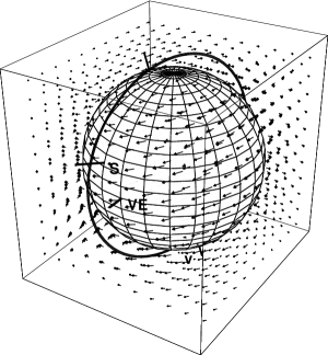
Figure 2: Shows the earth (N is up) and the much larger vorticity vector field component $\vec{\omega}$ induced by the translation of the earth, as in (34). The polar orbit of the GP-B satellite is shown, and ${\bf S}$ is the gyroscope starting spin orientation, directed towards the guide star IM Pegasi, RA = $22^{h}$ $53^{\prime}$ $2.26^{\prime\prime}$, Dec = $16^{0}$ $50^{\prime}$ $28.2^{\prime\prime}$, ${\bf VE}$ is the vernal equinox, and ${\bf V}$ is the direction $\mbox{RA}=5.2^{h}$, $\mbox{Dec}=-67^{0}$ of the translational velocity ${\bf v}_{c}$.

Here we consider one difference between the two theories, namely that associated with the vorticity part of (24), leading to the ‘frame-dragging’ or Lense-Thirring effect. In GR the vorticity field is known as the ‘gravitomagnetic’ field ${\bf B}=-c\>\vec{\omega}$. In both GR and the new theory the vorticity is given by (16) but with a key difference: in GR ${\bf v}_{R}$ is only the rotational velocity of the matter in the earth, whereas in (13)-(14) ${\bf v}_{R}$ is the vector sum of the rotational velocity and the translational velocity of the earth through the substratum. At least seven experiments have detected this translational velocity; some were gas-mode Michelson interferometers and others coaxial cable experiments [9, 10, 11], and the translational velocity is now known to be approximately 430 km/s in the direction RA $=5.2^{h}$, Dec$=-67^{0}$. This direction has been known since the Miller [13] gas-mode interferometer experiment, but the RA was more recently confirmed by the 1991 DeWitte coaxial cable experiment performed in the Brussels laboratories of Belgacom [10]. This flow is related to galactic gravity flow effects [9, 10, 11], and so is different to that of the velocity of the earth with respect to the Cosmic Microwave Background (CMB), which is $369$ km/s in the direction $\mbox{RA }=11.20^{h},\mbox{Dec }=-7.22^{0}$.

First consider the common but much smaller rotation induced ‘frame-dragging’ or vorticity effect. Then ${\bf v}_{R}({\bf r})={\bf w}\times{\bf r}$ in (16), where ${\bf w}$ is the angular velocity of the earth, giving

$$\vec{\omega}({\bf r})=4\frac{G}{c^{2}}\frac{3({\bf r}.{\bf L}){\bf r}-r^{2}{\bf L}}{2r^{5}},$$ (31)

where ${\bf L}$ is the angular momentum of the earth, and ${\bf r}$ is the distance from the centre. This component of the vorticity field is shown in Fig.1. Vorticity may be detected by observing the precession of the GP-B gyroscopes. The vorticity term in (23) leads to a torque on the angular momentum ${\bf S}$ of the gyroscope,

$$\vec{\tau}=\int d^{3}r\rho({\bf r})\;{\bf r}\times(\vec{\omega}({\bf r})\times{\bf v}_{R}({\bf r})),$$ (32)

where $\rho$ is its density, and where ${\bf v}_{R}$ is used here to describe the rotation of the gyroscope. Then $d{\bf S}=\vec{\tau}dt$ is the change in ${\bf S}$ over the time interval $dt$. In the above case ${\bf v}_{R}({\bf r})={\bf s}\times{\bf r}$, where ${\bf s}$ is the angular velocity of the gyroscope. This gives

$$\vec{\tau}=\frac{1}{2}\vec{\omega}\times{\bf S}$$ (33)

and so $\vec{\omega}/2$ is the instantaneous angular velocity of precession of the gyroscope. This corresponds to the well known fluid result that the vorticity vector is twice the angular velocity vector. For GP-B the direction of ${\bf S}$ has been chosen so that this precession is cumulative and, on averaging over an orbit, corresponds to some $7.7\times 10^{-6}$ arcsec per orbit, or 0.042 arcsec per year. GP-B has been superbly engineered so that measurements to a precision of 0.0005 arcsec are possible.

Figure 3: Predicted variation of the precession angle $\Delta\Theta=|\Delta{{\bf S}}(t)|/|{\bf S}(0)|$, in arcsec, over one 97 minute GP-B orbit, from the vorticity induced by the translation of the earth, as given by (35). The orbit time begins at location ${\bf S}$. Predictions are for the months of April, August, September and February, labeled by increasing dash length. The ‘glitches’ near 80 minutes are caused by the angle effects in (35). These changes arise from the effects of the changing orbital velocity of the earth about the sun. The GP-B expected angle measurement accuracy is 0.0005 arcsec. The gravitational waves will affect these plots, as shown in Fig.8 for 40 orbits.

However for the unique translation-induced precession if we use $v_{R}\approx v_{C}=430$ km/s in the direction $\mbox{RA}=5.2^{hr}$, $\mbox{Dec}=-67^{0}$, namely ignoring the effects of the orbital motion of the earth, the observed flow past the earth towards the sun, and the flow into the earth, and effects of the gravitational waves, then (16) gives

$$\vec{\omega}({\bf r})=\frac{2GM}{c^{2}}\frac{{\bf v}_{C}\times{\bf r}}{r^{3}}.$$ (34)

This much larger component of the vorticity field is shown in Fig.2. The maximum magnitude of the speed of this precession component is $\omega/2=gv_{C}/c^{2}=8\times 10^{-6}$arcsec/s, where here $g$ is the gravitational acceleration at the altitude of the satellite. This precession has a different signature: it is not cumulative, and is detectable by its variation over each single orbit, as its orbital average is zero, to first approximation. Fig.3 shows $\Delta\Theta=|\Delta{{\bf S}}(t)|/|{\bf S}(0)|$ over one orbit, where, as in general,

$$\Delta{{\bf S}}(t)=\int_{0}^{t}dt^{\prime}\frac{1}{2}\vec{\omega}({\bf r}(t^{\prime}))\times{\bf S}(t^{\prime})\approx\left(\int_{0}^{t}dt^{\prime}\frac{1}{2}\vec{\omega}({\bf r}(t^{\prime}))\right)\times{\bf S}(0).$$ (35)

Here $\Delta{{\bf S}}(t)$ is the integrated change in spin, and where the approximation arises because the change in ${\bf S}(t^{\prime})$ on the RHS of (35) is negligible. The plot in Fig.3 shows this effect to be some 30$\times$ larger than the expected GP-B errors, and so easily detectable. This precession is about the instantaneous direction of the vorticity $\vec{\omega}({\bf r}((t))$ at the location of the satellite, and so is neither in the plane, as for the geodetic precession, nor perpendicular to the plane of the orbit, as for the earth-rotation induced vorticity effect. This absolute motion induced spin precession is shown in Fig.4.

Because the yearly orbital rotation of the earth about the sun slightly effects ${\bf v}_{C}$ [10] predictions for four months throughout the year are shown in Fig.3. Such yearly effects were first seen in the Miller [13] experiment.

However the main new feature of this paper is the detailed prediction of the magnitude and signature of the new gravitational-wave induced spin precessions that GP-B is capable of detecting, but first we briefly summarise the history of the detection of gravitational waves.

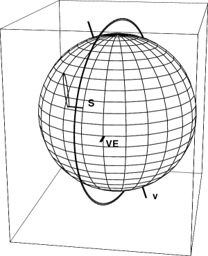
Figure 4: Predicted precession of the gyroscope spin axis, over one orbit of the satellite, but greatly exaggerated, directly manifesting the vorticity component of the flow caused by the translation of the earth, as in (34) and Fig.2. This component of the spin precession forms an elongated ellipse. Gravitational waves will cause changes in the size and orientation of this precession ellipse. The angle $\Delta\Theta$ in Fig.3 is the angle subtended at the earth’s centre by the starting position at ${\bf S}$ and a point on this ellipse of precession. The precession caused by the vorticity component arising from the rotation of the earth is perpendicular to the plane of the orbit, while the geodetic precession component is in the plane of the orbit. The polar orbit of the GP-B satellite is shown, and ${\bf S}$ is the gyroscope starting spin orientation, directed towards the guide star IM Pegasi, RA = $22^{h}$ $53^{\prime}$ $2.26^{\prime\prime}$, Dec = $16^{0}$ $50^{\prime}$ $28.2^{\prime\prime}$, ${\bf VE}$ is the vernal equinox, and ${\bf V}$ is the direction $\mbox{RA}=5.2^{h}$, $\mbox{Dec}=-67^{0}$ of the translational velocity ${\bf v}_{c}$.

7 Brief History of the Detection of Gravitational Waves

Figure 5: Variations in twice the one-way travel time, in ns, for an RF signal to travel 1.5 km through a coaxial cable between Rue du Marais and Rue de la Paille, Brussels. An offset has been used such that the average is zero. The definition of the sign convention for $\Delta t$ used by DeWitte is unclear. The cable has a North-South orientation, and the data is $\pm$ difference of the travel times for NS and SN propagation. The sidereal time for maximum effect of $\sim\!\!17$hr (or $\sim\!\!5$hr) (indicated by vertical lines) agrees with the direction found by Miller. Plot shows data over 3 sidereal days and is plotted against sidereal time in hours. The regular time variation is caused by the earth rotation changing the orientation of the cable with respect to the direction of absolute linear motion.

As already noted the velocity flow-field equations (13)-(14) have wave-like solutions involving variations in both the magnitude and direction of the velocity flow-field. Remarkably all the Michelson gas-mode interferometer and coaxial cable experiments showed evidence of such wave phenomena [10]. The first clear evidence was from the Miller 1925/26 experiment. Miller offered no explanation for these fluctuations but in his analysis of that data he did running time averages to remove these fluctuation effects, though some of that could also have been instrumental noise. While some of these fluctuations may also be partially caused by weather related temperature and pressure variations, the bulk of the fluctuations appear to be larger than expected from that cause alone. Even the original Michelson-Morley 1887 data shows variations in the velocity field and supports this interpretation. However it is significant that the non-interferometer 1991 DeWitte experiment also showed clear evidence of turbulence of the velocity flow field, as shown in Fig.7. Just as the DeWitte data agrees with the Miller data for speeds and directions of absolute motion, the magnitude of the fluctuations are also very similar [10]. It therefore becomes clear that there is strong evidence for these fluctuations being evidence of physical turbulence in the flow field. The magnitude of this turbulence appears to be larger than that which would be caused by the in-flow of quantum foam towards the sun, and indeed most of this turbulence may be associated with galactic in-flow into the Milky Way and local galactic cluster. This in-flow turbulence is a form of gravitational wave and the ability of gas-mode Michelson interferometers to detect absolute motion means that experimental evidence of such a wave phenomena has been available for a considerable period of time. All this means that the new gravitational wave phenomena is very easy to detect and amounts to new physics that can be studied in much detail.

Figure 6: Plot of the negative of the drift of the cross-over time between minimum and maximum travel-time variation each day (at $\sim 10^{h}\pm 1^{h}$ ST) versus local solar time for some 178 days. The straight line plot is the least squares fit to the experimental data, giving an average slope of 3.92 minutes/day. The time difference between a sidereal day and a solar day is 3.93 minutes/day. This demonstrates that the effect is related to sidereal time and not local solar time. The fluctuations apparent in the plot are caused by the slow changes in direction of the flow.

The DeWitte 1991 experiment within Belgacom, the Belgium telecommunications company, was a most impressive and high quality experiment that we now understand to have detected gravitational waves [10]. In this serendipitous discovery two sets of atomic clock in two buildings in Brussels, separated by 1.5 km, were used to time 5MHz radiofrequency signals travelling in each direction, through two buried coaxial cables, with a N-S orientation, linking the two clusters. The atomic clocks were cesium beam atomic clocks, and there were three in each cluster. In that way the stability of the clocks could be established and monitored. One cluster was in a building on Rue du Marais and the second cluster was due south in a building on Rue de la Paille. Digital phase comparators were used to measure changes in times between clocks within the same cluster and also in the propagation times of the RF signals. Time differences between clocks within the same cluster showed a linear phase drift caused by the clocks not having exactly the same frequency together with short term and long term noise. However the long term drift was very linear and reproducible, and that drift could be allowed for in analysing time differences in the propagation times between the clusters.

Changes in propagation times were observed and eventually observations over 178 days were recorded. A sample of the data, plotted against sidereal time for just three days, is shown in Fig.5. DeWitte recognised that the data was evidence of absolute motion but he was unaware of the Miller experiment and did not realise that the Right Ascension for minimum/maximum propagation time agreed almost exactly with Miller’s direction ($\alpha=5.2^{hr},\delta=-67^{0}$). In fact DeWitte expected that the direction of absolute motion should have been in the CMB direction, but that would have given the data a totally different sidereal time signature, namely the times for maximum/minimum would have been shifted by approximately 6 hrs. The declination of the velocity observed in this DeWitte experiment cannot be determined from the data as only three days of data are available. However assuming exactly the same declination as Miller the speed observed by DeWitte appears to be also in excellent agreement with the Miller speed, which in turn is in agreement with that from the Michelson-Morley and Illingworth experiments [10].

Importantly DeWitte reported the sidereal time of the cross-over time, that is a ‘zero’ time in Fig.5, for 178 days of data. This is plotted in Fig.6 and demonstrates that the time variations are correlated with sidereal time and not local solar time. A least squares best fit of a linear relation to that data gives that the cross-over time is retarded, on average, by 3.92 minutes per solar day. This is to be compared with the fact that a sidereal day is 3.93 minutes shorter than a solar day. So the effect is certainly cosmological and not associated with any daily thermal effects, which in any case would be very small as the cable is buried. Miller had also compared his data against sidereal time and established the same property, namely that up to small diurnal effects identifiable with the earth’s orbital motion, features in the data tracked sidereal time and not solar time.

If the changes in propagation time through the coaxial cable were caused solely by the rotation of the coaxial cable, carried along by the rotation of the earth, so changing its orientation with respect to that of a uniform absolute velocity, then the variations in travel time would not show the fluctuations that are evident in Fig.5, but only the dominant regular variation over each sidereal day. So these fluctuations, and they are much larger than any errors that were produced by the atomic clock timing procedures, are manifestations of a genuine novel physical effect. Here and in [9, 10] they are interpreted as the gravitational waves predicted by the theory in Sect.5. By fitting the data to the time variation forms expected without such fluctuations, the fluctuations themselves may extracted and their magnitude translated into speed variations, as shown in Fig.7.

Figure 7: Speed fluctuations determined from Fig.5 over three sidereal days, or some 70 hours. A 1ns variation in travel time corresponds approximately to a speed variation of 27km/s. The larger speed fluctuations are anomalies of the fitting technique and actually arise from a fluctuation in the cross-over time, that is, a fluctuation in the direction of the velocity.

As well Torr and Kolen in 1984 also used a coaxial cable experiment to detect absolute motion [10]. Unfortunately the cable was orientated in an E-W direction, which made it relatively insensitive to the detection of absolute motion, as that is in a near N-S direction, though the expected travel variations were indeed observed [10]. However being in the E-W direction the Torr-Kolen coaxial cable is very sensitive to the directional changes associated with the turbulence. Being almost at $90^{0}$ to the direction of absolute motion, any variation in that direction produces significant effects, as indeed reported by Torr and Kolen. So we have yet another experiment in which the data is such that we have interpreted it as the detection of these new gravitational waves.

Figure 8: Predicted variation of the precession angle $\Delta\Theta=|\Delta{{\bf S}}(t)|/|{\bf S}(0)|$, in arcsec, as given by (35), over 40 GP-B orbits, from the vorticity induced by the absolute linear motion of the earth, and with the mainly galactic gravitational waves now included by means of the simulation described in the text. This plot shows the expected magnitude and signature of the effects of the gravitational waves. The corresponding prediction for one orbit, but without the gravitational wave effect, is shown in Fig.3. The main signature of the gravitational waves for GP-B is the variation, from orbit to orbit, of the maximum precession angle, as shown in this plot. The orbit time begins at location ${\bf S}$ in Fig.3. Predictions are for the month of September. The GP-B expected angle measurement accuracy is 0.0005 arcsec.

8 Detection of Gravitational Waves by GP-B

The novel gravitational waves displayed in Fig.7 are significant in magnitude compared to the average absolute motion speed of some 430 km/s. For that reason they have a significant effect upon the vorticity field, and consequently of the GP-B spin precessions. To give a first indication of the expected size of these wave induced spin precessions we have used the speed magnitude fluctuations in Fig.7 by simply adding these fluctuations to the speed of 430 km/s in the direction RA $=5.2^{h}$, Dec$=-67^{0}$, but without allowing for any fluctuation in direction. Then the spin precession in (35) was integrated over 40 orbits of the satellite, with the results shown in Fig.8 for September. This figure should be compared with the form in Fig.3 for only one orbit, and without the gravitational wave effect. We see the magnitude and signature of the gravitational wave induced spin precessions, including the effect that the absolute motion induced precessions now no longer return to zero after each orbit. Whether this effect persists over many months is not possible to predict, but if it did persist then it would seriously interfere with, in particular, the observation of the earth-rotation induced spin precession, which is cumulative but very small.

There is a technical difficulty in observing the effects shown in Figs.3 and 8, namely that the guide star is not visible to the on-board GP-B telescope during the ‘mid-part’ of each orbit, as is apparent from Fig.2.

9 Conclusions

By using the gravitational wave effects revealed by the DeWitte coaxial cable absolute linear motion experiment we have been able to simulate the effects of these waves upon the spin precession of the GP-B gyroscopes, in order that the signature of these effects may be recognised in the GP-B data. Both the absolute linear motion and the new gravitational waves are properties of the new theory of space and gravity. These effects are absent from General Relativity, and which, most significantly, has had only one observational test, namely the binary pulsar slow-down, so far, of its dynamical properties, as distinct from the various tests of the geodesic equation. The new theory of gravity has explained a number of observational and laboratory effects, but in particular it has explained the so-called ‘dark matter’ effect as a dynamical property of space itself; so it is not caused by any form of ‘matter’. So the ‘dark matter’ effect was a fatal flaw of General Relativity. As well the spacetime ontology, as distinct from the mathematical formalism, is also seriously flawed by the fact that so far at least seven experiments have detected absolute linear motion. The GP-B experiment will also detect evidence of this absolute motion because of the vorticity associated with that motion, that is, caused by the earth passing through space, which includes also a much smaller vorticity caused by the earth’s rotation. This component is identical to the vorticity caused by the earth’s rotation within General Relativity. So General Relativity is in the paradoxical situation of permitting absolute rotational motion but banning absolute linear motion. One major outcome of the GP-B experiment will be the definitive resolution of this longstanding paradox.

References

- [1] G. Pugh, in Nonlinear Gravitodynamics: The Lense - Thirring Effect, eds. R. Ruffini and C. Sigismondi, World Scientific Publishing Company, 2003, pp 414-426, (Based on a 1959 report).
- [2] L.I. Schiff, Phys. Rev. Lett. 4, 215(1960).
- [3] R.A. Van Patten and C.W.F. Everitt, Phys. Rev. Lett. 36, 629(1976).
- [4] C.W.F. Everitt et al., in: Near Zero: Festschrift for William M. Fairbank, ed. C.W.F. Everitt, (Freeman Ed,. S. Francisco, 1986).
- [5] J.P. Turneaure, C.W.F. Everitt, B.W. Parkinson, et al., The Gravity Probe B Relativity Gyroscope Experiment, in Proc. of the Fourth Marcell Grossmann Meeting in General Relativity, ed. R. Ruffini, (Elsevier, Amsterdam, 1986).
- [6] R.T. Cahill, ‘Dark Matter’ as a Quantum Foam In-Flow Effect, in Progress In Dark Matter Research, (Nova Science Pub., NY to be pub. 2004), physics/0405147; R.T. Cahill, Gravitation, the ‘Dark Matter’ Effect and the Fine Structure Constant, physics/0401047.
- [7] R.T. Cahill, Novel Gravity Probe B Frame-Dragging Effect, physics/0406121.
- [8] M.E. Ander et al., Phys. Rev. Lett. 62, 985(1989).
- [9] R.T. Cahill, Quantum Foam, Gravity and Gravitational Waves, in Relativity, Gravitation, Cosmology, pp. 168-226, eds. V. V. Dvoeglazov and A. A. Espinoza Garrido, (Nova Science Pub., NY, 2004).
- [10] R.T. Cahill, Absolute Motion and Gravitational Effects, Apeiron, 11, No.1, pp. 53-111(2004).
- [11] R.T. Cahill, Process Physics: From Information Theory to Quantum Space and Matter, (Nova Science Pub., NY to be pub. 2004), in book series Contemporary Fundamental Physics, ed. V.V. Dvoeglazov.
- [12] R.T. Cahill, The Dynamical Velocity Superposition Effect in the Quantum-Foam In-Flow Theory of Gravity, physics/0407133.
- [13] D.C. Miller, Rev. Mod. Phys. 5, 203-242(1933).