Angular momentum of a strongly focussed Gaussian beam

Abstract

A circularly polarized rotationally symmetric paraxial laser beams carries $\pm\hbar$ angular momentum per photon as spin. Focussing the beam with a rotationally symmetric lens cannot change this angular momentum flux, yet the focussed beam must have spin $|S_{z}|<\hbar$ per photon. The remainder of the original spin is converted to orbital angular momentum, manifesting itself as a longitudinal optical vortex at the focus. This demonstrates that optical orbital angular momentum can be generated by a rotationally symmetric optical system which preserves the total angular momentum of the beam.

I Introduction

That optical and other electromagnetic fields can carry angular momentum is a direct result of the fact that they can carry linear momentum. Since the linear momentum flux density of an electromagnetic field is $\mathbf{E}\times\mathbf{H}/c$, giving

$$\mathbf{p}=\frac{1}{2c}\mathrm{Re}(\mathbf{E}\times\mathbf{H}^{\ast})$$ (1)

for the time-averaged momentum flux density of a time-harmonic electromagnetic beam, it is tempting to write

$$\mathbf{j}=\frac{1}{2c}\mathrm{Re}(\mathbf{r}\times(\mathbf{E}\times\mathbf{H}^{\ast})).$$ (2)

as the corresponding angular momentum flux density. However, since the conservation law for linear momentum only contains the time-derivative of the momentum density, and the divergence of the flux (or the volume integrals of these, noting that the volume integral of a divergence of a quantity can be written as the surface integral of the quantity), it is premature to identify this as the actual angular momentum flux density. If the above expression was in fact the correct angular momentum flux density, then the angular momentum of a circularly polarized plane would be zero. Since the correct classical angular momentum density must agree with the classical limit of the quantum angular momentum density, this must be incorrect. This was recognized long ago, and a separation of the angular momentum of the field can be separated into spin and orbital components yields a result in agreement with the quantum result Humblet (1943); van Enk and Nienhuis (1994); Crichton and Marston (2000).

The total momentum or angular momentum flux through a plane can be unambiguously determined by integrating the above quantities over the plane; this is a straightforward application of the integral form of the conservation law for angular momentum, and is therefore independent of the actual choice of expression for the angular momentum density. It can be noted that the actual momentum and angular momentum densities (as opposed to the flux densities given above) contain an extra $1/c$ factor, and can be integrated over the whole beam to give the total momentum and angular momentum content. However, for the case of an infinitely long beam, these quantities are infinite, and it is better to consider only the fluxes.

Separating the total angular momentum flux of the beam into spin and orbital components gives

$$\mathbf{J}=\mathbf{L}+\mathbf{S}$$ (3)

where the total angular momentum flux $\mathbf{J}$ is the sum of an orbital term $\mathbf{L}$ and a spin term $\mathbf{S}$. A similar relationship exists for the angular momentum flux densities and densities at any point. The distinction is simply that the spin angular momentum density is independent of the choice of origin; that is, it is invariant with respect to translations of the coordinate system. Since the local conservation of angular momentum as the beam propagates in free space cannot depend on the choice of the origin of the coordinate system, both the orbital and spin components must be individually conserved, as well as the total angular momentum, since there would otherwise exist a choice-of-origin dependent torque exerted by the beam on free space. These quantities can only change if the field interacts with matter van Enk and Nienhuis (1994).

In general, the separation into spin and orbital components is not quite as straightforward as one might hope Humblet (1943); van Enk and Nienhuis (1994); Crichton and Marston (2000). One can, however, write expressions for the spin and orbital components. The Cartesian components of the time-averaged spin angular momentum flux density $\mathbf{s}$ are Humblet (1943); van Enk and Nienhuis (1994); Crichton and Marston (2000)

$$s_{x} = \epsilon_{0}\mathrm{Im}(E_{y}E_{z}^{\star})/\omega$$

$$s_{y} = \epsilon_{0}\mathrm{Im}(E_{x}^{\star}E_{z})/\omega$$ (4)

$$s_{z} = \epsilon_{0}\mathrm{Im}(E_{x}E_{y}^{\star})/\omega$$

where $E_{x,y,z}$ are the Cartesian components of $\mathbf{E}$, the complex vector amplitude. This result can also be written in terms of the Levi–Civita symbol as $s_{i}=\mathrm{i}\epsilon_{0}\epsilon_{ijk}E_{j}E_{k}^{\star}/(2\omega)$, where the expression is summed over repeated indices and the real part is taken. The orbital components are Humblet (1943); van Enk and Nienhuis (1994); Crichton and Marston (2000)

$$l_{i}=\mathrm{i}\epsilon_{0}E_{j}(\mathbf{r}\times\nabla)E_{j}^{\star}/(2\omega).$$ (5)

These give simple results for paraxial beams. For example, a circularly polarized paraxial beam of power $P$ and frequency $\omega$ has a spin angular momentum flux of $\pm P/\omega$, depending on the handedness of the polarization Jackson (1999). This result is equivalent to the quantum mechanical result of $\pm\hbar$ per photon. If the beam has a uniform phase over a plane, or, more generally, phase that is rotationally symmetric about the beam axis, then the orbital angular momentum flux density is zero.

We will consider such rotationally symmetric beams here, and present specific results for a Gaussian beam.

II Angular momentum of a finite beam

The case of spin angular momentum flux equal to $P/\omega$ results only in the paraxial approximation, as it depends on $E_{z}$ being zero. If we consider a beam of finite width in its focal plane, then the beam will spread through diffraction, and will, at a sufficiently large distance, be propagating in a purely radial direction. That is, for large $r$, we must have $E_{r}=0$. In this case, the electric field is purely tangential, and the spin angular momentum density in polar spherical coordinates is

$$s_{r}=\epsilon_{0}\mathrm{Im}(E_{\theta}E_{\phi}^{\star})/\omega,$$ (6)

with the other vector components being zero. For a rotationally symmetric beam of the type we consider here, $s_{r}$ will be independent of the azimuthal angle $\phi$.

Therefore, the maximum possible contribution to the total spin angular momentum, of which, by symmetry, only the $z$ component is non-zero, is $s_{r}\cos\theta$, where $\theta$ is the angle measured from the $z$ axis. Integrating this over the beam must result in $|S_{z}|<\hbar$ per photon. A consequence of this is that a focussed beam cannot be purely circularly polarized everywhere in a plane, including the focal plane. If the beam is rotationally symmetric and locally circularly polarized in the far field, the beam cannot be partially plane polarized in the focal plane, either—therefore, the electric field must have an axial component ($E_{z}\neq 0$). A similar argument using linear momentum shows that plane polarized beams must have $E_{z}\neq 0$ in the focal plane as well.

As an example, we will find the spin carried by a focussed Gaussian beam. A paraxial Gaussian beam has a (scalar) amplitude in the far field of

$$U=U_{0}\exp\left[-\frac{k^{2}w_{0}^{2}\tan^{2}\theta}{4}\right]$$ (7)

where $k$ is the wavenumber and $w_{0}$ is the paraxial beam waist radius Nieminen et al. (2003), or in terms of the beam convergence angle given by $\tan\theta_{0}=2/(kw_{0})$,

$$U=U_{0}\exp(-\tan^{2}\theta/\tan^{2}\theta_{0}).$$ (8)

For maximum possible spin, we have $s_{r}=\epsilon_{0}U^{2}/\omega$, and the total spin angular momentum of the beam, in units of $\hbar$ per photon, can be found by integrating over a hemisphere:

$$S_{z}=A/P$$ (9)

where

$$A=\int_{0}^{\pi/2}\exp(-2\tan^{2}\theta/\tan^{2}\theta_{0})\sin\theta\cos\theta\mathrm{d}\theta$$ (10)

and

$$P=\int_{0}^{\pi/2}\exp(-2\tan^{2}\theta/\tan^{2}\theta_{0})\sin\theta\mathrm{d}\theta.$$ (11)

This can be readily integrated numerically, and the result for all practically realizable Gaussian beams is shown in figure 1. The qualitative behaviour seen here is expected since $S_{z}=0.5P/\omega$ for a dipole radiation field Crichton and Marston (2000).

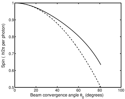
Figure 1: Spin angular momentum in $\hbar$ per photon for a non-paraxial TEM₀₀ Gaussian beam. The solid line shows the exact result, the dotted line shows the small-angle approximation.

For $\theta_{0}\ll 1$, small angle approximations can be made, giving

$$S_{z}=1-\theta_{0}^{2}/4.$$ (12)

The relative error in the change in spin ($1-S_{z}$) is less than $0.01$ for beam convergence angles $\theta_{0}<6.25^{\circ}$, and less than $0.1$ for $\theta_{0}<21^{\circ}$.

Although the spin angular momentum flux of the beam is reduced by the beam being focussed, a lossless rotationally symmetric optical system cannot change the total angular momentum flux of an electromagnetic field Waterman (1971). Therefore, there must be a corresponding increase in the orbital angular momentum. This is in remarkable contrast to the usual methods of generating optical vortices which employ astigmatic or cylindrical lenses or holograms designed to break the rotational symmetry. The key difference is that orbital angular momentum generation by focussing depends on the initial presence of spin angular momentum, whereas astigmatic systems do not.

An interesting question that remains to be answered is in what way the focussed beam carries the orbital angular momentum. This is best addressed by considering a rigorous electromagnetic model of the beam.

II.1 Multipole expansion

A time-harmonic electromagnetic beam can be represented as a sum of of electric and magnetic multipoles:

$$\mathbf{E}(\mathbf{r})=\sum_{n}^{\infty}\sum_{m=-n}^{n}a_{nm}\mathbf{M}_{nm}+b_{nm}\mathbf{N}_{nm}$$ (13)

where $\mathbf{M}_{nm}$ and $\mathbf{M}_{nm}$ are the TE and TM regular multipole fields, or vector spherical wavefunctions Nieminen et al. (2003). Not only are these wavefunctions a complete orthogonal set of divergence-free solutions of the vector Helmholtz equation (and hence solutions to the Maxwell equations), they are also eigenfunctions of the angular momentum operator $J^{2}$, with eigenvalues $[n(n+1)]^{1/2}$, and $J_{z}$, with eigenvalues $m$. The spin and orbital contributions to the anglular momentum can be calculated from the expansion coefficients $a_{nm}$ and $b_{nm}$ Crichton and Marston (2000); Bishop et al. (2003).

The only non-zero multipole coefficients for a left-circularly polarized rotationally symmetric beam are those with $m=1$. Thus, the total angular momentum about the $z$ axis is $\hbar$ per photon. The multipole expansion coefficients for the beam can be determined by an overdetermined point-matching method Nieminen et al. (2003). For a beam of finite width, it is found that the total spin is less than $\hbar$ per photon (spin calculated in this way exactly reproduces the curve in figure 1). The remainder of the angular momentum is orbital.

Since the multipole expansion of the beam is known, the fields can be calculated at any point in space. The components of the electric field in the focal plane are shown in figure 2. For a strongly focussed beam such as is shown in figure 2, the longitudinal (ie $z$) component of the field is significant, with a magnitude of $\approx 0.3$ times the transverse components. All components of the electric field show secondary diffraction rings (note that the radial dependence of multipole fields includes a spherical Bessel function). The phases of the $x$ and $y$ components are uniform, except for an increment of $\pi$ between successive diffraction rings, and, due to the circular polarization, differ by $\pi/2$ from each other. The phase of the $z$ component, however, shows a clear azimuthal dependence identical to that seen in $l=1$ paraxial vortex modes. Since this vortex behaviour is only possessed by the longitudinal component of the field, this can be called a longitudinal optical vortex.

Calculation of the Poynting vector shows that there is indeed a transverse component, which, since its handedness is uniform, is responsible for the transport of the orbital angular momentum.

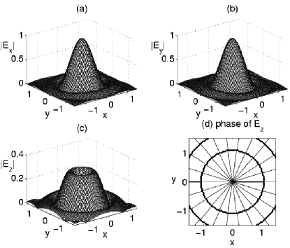
Figure 2: Electric field components of a strongly focussed circularly polarized Gaussian beam, with a convergence angle of 45^∘. The $x$, $y$, and $z$ components of the electric field in the focal plane are shown in (a), (b), and (c), while (d) shows phase contours (with a spacing of $2\pi/20$) for the $z$ component, showing azimuthal variation of phase as seen in vortex beams.

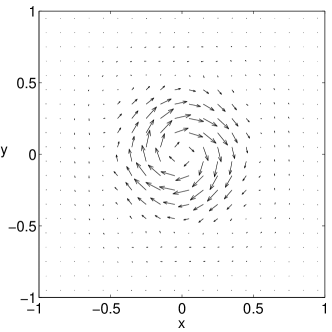
Figure 3: Poynting vector of a strongly focussed circularly polarized Gaussian beam, with a convergence angle of 45^∘. The transverse part ($x$ and $y$ components) of the Poynting vector in the focal plane are shown.

As the beam is more strongly focussed, the magnitude of the longitudinal ($z$) component of the field increases, and the orbital angular momentum increases as a result. The same increase can also be considered to result from the decrease of spin angular momentum, along with the conservation of total angular momentum. The change in the angular momentum and the growth of the longitudinal optical vortex is smooth and well-behaved as the convergence angle of the beam is increased, with no sudden qualitative or quantitative changes. As the beam is more strongly focussed, the diffraction rings also become more prominent, but this does not affect the angular momentum of the beam.

III Discussion

III.1 Torque density acting on lens

In light of the above considerations, the transformation of spin angular momentum to orbital angular momentum by the lens must result in a reaction torque density about the $z$-axis acting on the lens that depends on the choice of origin. While such a torque acting on empty space is unacceptable on physical grounds, it is not only entirely reasonable, but expected, in the case of a lens.

One need only to consider a simple ray picture of the action of a lens, not centered on the $z$ axis, on a ray parallel to the $z$-axis. The focussed ray will generally not pass through the $z$-axis, and is not parallel to the $z$-axis, and hence carries orbital angular momentum about the $z$-axis. Consequently, there must be a reaction torque density acting on the lens. Note that this torque density depends on the choice of origin. The component about any axis parallel to the beam axis of the total torque acting on the lens is, of course, zero.

III.2 Rotation in optical traps

The presence of orbital angular momentum in the focal region suggests that orbital motion of absorbing or reflective spherical particles should be observable in optical tweezers. However, since particles trapped in a Gaussian beam trap will be located on the beam axis, all that will be observed will be spinning of the particle about its axis. In order to observe this orbital angular momentum, it would be necessary to use a multi-ringed beam with zero orbital angular momentum, for example a Laguerre-Gauss mode LG_p0, with $p>1$, or a Bessel beam, as the input to the objective lens of the trap. In this case, particles trapped in one of the rings rather than the central spot can be be expected to undergo orbital motion.

IV Conclusion

We note that focusing a circularly polarized beam preserves the total angular momentum flux of the beam about its axis. However, the spin component of the angular momentum flux is necessarily reduced as the beam is more strongly focussed. Due to the conservation of total angular momentum when the beam is focussed by a rotationally symmetric optical system, there must be a corresponding increase in the orbital angular momentum flux. This result is remarkable in that it predicts the generation of orbital angular momentum by a rotationally symmetric optical system, in apparent contradiction with common expectation.

This orbital angular momentum is carried by the axial component of the electric field, $E_{z}$, which has the typical $\exp(\mathrm{i}\phi)$ dependence of charge 1 optical vortices; we call this a longitudinal optical vortex.

References

- Humblet (1943) J. Humblet, Physica 10, 585 (1943).
- van Enk and Nienhuis (1994) S. J. van Enk and G. Nienhuis, J. Mod. Opt. 41, 963 (1994).
- Crichton and Marston (2000) J. H. Crichton and P. L. Marston, Electronic Journal of Differential Equations Conf. 04, 37 (2000).
- Jackson (1999) J. D. Jackson, Classical Electrodynamics (John Wiley, New York, 1999), 3rd ed.
- Nieminen et al. (2003) T. A. Nieminen, H. Rubinsztein-Dunlop, and N. R. Heckenberg, J. Quant. Spectrosc. Radiat. Transfer 79-80, 1005 (2003).
- Waterman (1971) P. C. Waterman, Physical Review D 3, 825 (1971).
- Bishop et al. (2003) A. I. Bishop, T. A. Nieminen, N. R. Heckenberg, and H. Rubinsztein-Dunlop, Phys. Rev. A 68, 033802 (2003).