Determination of the characteristic directions of lossless linear optical elements

Abstract

We show that the problem of finding the primary and secondary characteristic directions of a linear lossless optical element can be formulated in terms of an eigenvalue problem related to the unimodular factor of the transfer matrix of the optical device. This formulation makes any actual computation of the characteristic directions amenable to pre-implemented numerical routines, thereby facilitating the decomposition of the transfer matrix into equivalent linear retarders and rotators according to the related Poincaré equivalence theorem. We explain in detail how this issue arises in the context of stress analysis based on integrated photoelasticity or hybrid methods combining photoelastic measurements with analytical stress models and/or numerical Finite-Element computations for the stress tensor field. Furthermore we show how our results can be applied when algorithms for the reconstruction of the dielectric tensor in the interior of a photoelastic model (dielectric tensor imaging) are tested for their stability against noise in the measurement data. For the sake of completeness we provide a brief derivation of the basic equations governing integrated photoelasticity.

Keywords: Equivalent optical model. Poincaré Equivalence Theorem. Integrated Photoelasticity. Dielectric tensor imaging. Stability of reconstruction algorithms.

I Introduction

Passive linear optical elements are ubiquitous in the study of interactions between matter and polarized classical Born and Wolf (1999); Longhurst (1973); Ditchburn (1976); Hecht (1998); Guenther (1990) or quantum light Leonhardt (2003). While polarizers attenuate one of two distinguished orthogonal polarization forms, linear retarders and rotators alter the state of polarization while preserving the flow of light energy through the device. The latter two belong to the class of non-absorbing linear elements, where the term “linear” refers to the fact that the action of such a device on the state of polarization can be conveniently described by a unitary two-by-two transfer matrix. In contrast, a polarizer would be represented by a Hermitean matrix. This description of linear optical elements in terms of Hermitean and unitary matrices is called the Jones formalism Jones (1941a); Hurwitz and Jones (1941); Jones (1941b, 1942, 1947a, 1947b, 1948, 1956a, 1956b).

In his treatise on classical light Poincaré (1892), Poincaré found that any non-absorbing passive linear optical element could be decomposed into basic linear retarders and rotators. By linear retarder we mean a homogeneously anisotropic device, such as a piece of appropriately cut crystal, which possesses two preferred axes, called the “fast” and “slow” axis, which are perpendicular to each other and differ in the phase velocity of component waves linearly polarized along the distinguished directions; as a consequence, light possessing a general elliptic polarization state will accumulate a relative phase retardation between the two components and thus change its polarization form. A rotator, on the other hand, changes the plane of linearly polarized light by a specified angle; it can be shown easily that this effect is due to a phase retardation between the two orthogonal components of circular polarization. Accordingly, a linear retarder is determined by specification of, e.g., the angle of the fast axis, and the relative phase retardation; while a single rotation angle is sufficient to specify a rotator. This decomposition of a general non-absorbing optical element into retarders and rotators is called the Poincaré equivalence theorem (see Ref. Hammer (2004) for a recent account).

Such a decomposition proves very useful whenever the determination of the internal stress tensor of a transparent medium by means of non-destructive methods is desired. This issue arises in the following context: material scientists and engineers wish to gain insight into the stress and strain fields in the interior of a loaded specimen. Amongst the many different approaches, three methods are most often used: (1) an educated guess at the analytic mathematical form of the internal stress or strain tensor is made; (2) the external load acting on the specimen is systematically approximated by forces applying on finitely many points on the surface of the object; and the resulting stress in the interior is then computed using numerical schemes generically called Finite Element Methods (FEM) Cook (1994); Holand and Bell (1969); Dankert and Dankert (2004); (3) the phenomenon of photoelasticity is utilized to gain insight into the internal stress distribution. The term photoelasticity refers to the fact that some transparent materials, typically resins or glasses, become birefringent when under external load, while being optically isotropic in the unloaded state. Within certain limits, the relation between the dielectric tensor $\epsilon_{ij}$ and the stress tensor $\sigma_{ij}$ is linear, and is generically called a stress-optical law. Its typical form has been given long ago by Maxwell Maxwell (1853),

$$\epsilon_{ij}=\epsilon\,\delta_{ij}+C_{1}\,\sigma_{ij}+C_{2}\,\operatorname{tr}{\sigma}\,\delta_{ij}\quad,$$ (1)

where $C_{1},C_{2}$ are called stress-optical constants. This one-to-one relation between dielectric tensor and stress tensor suggests that one builds a model of an industrial component from an appropriate material (today, plastics are usually used) and loads the model just as the real object. The model is then subjected to heat, so as to loosen, and rearrange, the molecular bonds in the material; and subsequently cooled down, or “stress-frozen”, upon which the stress pattern remains locked inside the material Frocht (1941, 1948); Coker and Filon (1957). To determine these patterns, destructive and non-destructive methods are available.

A particular example of non-destructive evaluation has been termed “Integrated Photoelasticity” Aben (1966). Here, polarized light is sent through the specimen at many different angles, and the change in polarization form is registered for each light ray (pixelwise), utilizing appropriate combinations of polariscopes and digital cameras. To each ray passing through a specified point, and along a specified direction, a unitary transfer matrix $U$ can be assigned, which describes how the polarization form changes along the given ray. In this way we obtain a map from the set of all (reasonably smooth) dielectric tensor, or stress tensor, fields in the interior of the specimen, to the collection of transfer matrices, gathered for all necessary points and directions. In the theory of Inverse Problems and Mathematical Tomography Kirsch (1996); Denisov (1999); Bukhgeim (1999); Helgason (1980); Natterer (1986); Engl et al. (2000), this map is commonly called the forward problem. The associated inverse problem consists of reconstructing the interior dielectric tensor, or stress tensor, from a given collection of transfer matrices.

The transfer matrices $U$ are not observable directly. Rather, they are known functions of the global phase of the light beam, and three so-called “characteristic parameters” Aben (1966), two of which may be regarded as polarization directions, while the third one has the meaning of a “characteristic phase retardation”. Their operational meaning is as follows: the primary characteristic directions determine those planes of linear polarization at the entry into the medium for which the state of polarization of the emergent beam is again linear. The secondary characteristic directions determine the planes of linear polarization of the emerging light, if the incident light was linearly polarized in the primary characteristic directions; in general, they differ from the primary ones. There are always two orthogonal primary and two orthogonal secondary characteristic directions such that light which is linearly polarized along the two primary directions travels with different phase velocities. As a consequence, both waves emerge with a phase difference—the characteristic phase retardation. The characteristic parameters Aben (1966) of a linear lossless device are usually taken to be simple linear combinations of the angles specifying one of the primary characteristic directions, and the angle of the associated secondary characteristic direction; and the characteristic phase retardation (see section IV).

Traditionally, the forward problem in integrated photoelasticity is formulated directly in terms of the bulk stress tensor; however, more recent attempts Hammer and Lionheart (2005) have shown that it may be advantageous to first determine the dielectric tensor inside the model by tomographic means, after which the stress tensor can be computed via the stress-optical law in eq. (1). The solution to the inverse problem for the two-dimensional (2D) case, i.e., when the specimen is a thin slab, and the stress tensor inside possesses only two principal directions, is known long since Frocht (1941, 1948); Coker and Filon (1957); Theocaris and Gdoutos (1979); Ditchburn (1976); Aben (1966, 1979); Aben and Guillemet (1993); Aben et al. (1989). The general solution to the three-dimensional (3D) inverse problem is not known to date, although it has been shown recently Hammer and Lionheart (2005) that, in the limit of weak optical anisotropy, the 3D inverse problem can be mathematically reduced to six independent 2D inverse problems.

Being one of the oldest methods of experimental stress analysis, photoelasticity has been somewhat overshadowed by FEM methods over the past two or three decades, but has seen a recent revival with applications in silicon wafer stress analysis, rapid prototyping, fiber optic sensor development, and image processing Asundi (1996). As photoelasticity can be regarded as a natural complement to FEM numerics, hybrid methods attempting at combining both approaches are becoming popular. It then becomes a viable task to compare FEM results with those obtained by photoelastic tomography.

These considerations describe the context in which the method of determining the characteristic directions of a linear optical element, as given in this paper, is expected to prove useful. Specifically, there are four applications of our results in integrated photoelasticity and associated hybrid methods:

1. Testing the validity of analytic stress models: Here, we start with an educated guess about the analytic form of the bulk stress tensor field; then compute the associated dielectric tensor via the stress-optical law in eq. (1); and use this to compute the transfer matrices of the forward problem numerically, using eq. (12) in section II below. In order to facilitate a comparison with the characteristic parameters obtained from a direct photoelastic evaluation of a stress-frozen model, a decomposition of the numerically obtained transfer matrices into equivalent retarders and rotators must be performed for each light ray. Such a decomposition has to evaluate the characteristic directions of a given transfer matrix $U$ first; subsequently, the associated characteristic phase retardation follows automatically, as will be shown in section III. It is here where our method of determining the characteristic directions is needed.

2. Testing the validity of a FEM-based calculation: instead of an analytic stress model we might want to compare a bulk stress tensor field evaluated numerically using FEM, with photoelastic data. As in the last item, the stress tensor leads to a dielectric tensor and subsequently to a collection of numerically computed transfer matrices via the forward problem, eq. (12). Again, the comparison with actual measurements made on a photoelastic specimen requires the decomposition of these transfer matrices according to the equivalent optical model.

3. Iterative solutions of the inverse problem in integrated photoelasticity: the integral equation (12) determining the transfer matrices in terms of the dielectric tensor field is non-linear; this accounts for the fact that the full solution to the general 3D inverse problem of determining the dielectric tensor in terms of the transfer matrices is not yet known. Iterative numerical schemes to solve eq. (12) for $\epsilon_{ij}$ may be conceived. At each stage of iteration, the intermediate result for the dielectric tensor can be used to compute a collection of associated transfer matrices, whose characteristic parameters, in turn, may be compared with actual photoelastic data in order to check the convergence of the iterative algorithm. At this last stage we again need the decomposition of a given transfer matrix in terms of the equivalent optical model.

4. Stability of inversion algorithms on noisy data: the reliability of a reconstruction depends on how stable the algorithm is with respect to finite errors in measurement data. This stability can be tested on artificial analytic stress models, as follows: the stress model can be converted into a collection of transfer matrices as explained in item 1.) above. We then decompose each $U$ into characteristic parameters ; but instead of feeding these data directly into the inversion we subsequently add some numerical noise to the characteristic parameters, thus simulating errors in the measuring apparatus. These modified data are then fed into the proposed algorithm to check how far the new reconstruction deviates from the one without noise in the data. A visual example of this procedure is given in Fig. 1 for a standard reconstruction algorithm (filtered back-projection Natterer (1986)).

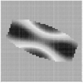
(a)

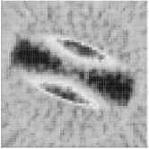
(b)

Figure 1: A cylinder is subject to axial load; the resulting deformation is modelled as a simulated displacement field on the surface and in the interior. Hooke’s law gives the relation between the resulting strain and stress tensors; from the stress-optical law, eq. (1), the dielectric tensor is then obtained. This is an example of an artificial stress model giving rise to a simulated dielectric tensor which can be used to test photoelastic reconstruction algorithms as follows: a plane intersecting the cylinder at an angle of $22^{\circ}$ relative to the symmetry axis of the cylinder is chosen in the figure. The unit normal vector to this plane is $\bm{\eta}$. The component of the dielectric tensor in the direction of $\bm{\eta}$ is $\epsilon_{\eta\eta}=\epsilon(\bm{\eta},\bm{\eta})$. In subfigure (a), its relative deviation $(\epsilon_{\eta\eta}-\epsilon)/\epsilon=A_{\eta\eta}$ from the scalar isotropic value $\epsilon$ is plotted. In subfigure (b), the simulated dielectric tensor $\epsilon_{ij}$ is used to compute a collection of transfer matrices $U$ via the forward problem, eq. (12). The transfer matrices are then decomposed according to the equivalent optical model, using the method introduced in section III; subsequently, Gaussian noise is imposed on the characteristic parameters, eq. (37), thus simulating measurement errors. The noisy parameters then recombine, again via the equivalent optical model, to give new, “noisy”, transfer matrices, from which the “noisy” dielectric tensor can be reconstructed via a filtered back-projection algorithm Natterer (1986); Engl et al. (2000). The result of this reconstruction, for $60\times 60$ pixels and $90$ scans around the object, is plotted in subfigure (b). It is seen that the noise in the characteristic parameters, and the noise in the global phase $\phi$, eq. (16), give rise to a halo-like pattern around the object, in addition to the speckled appearance of the reconstruction. – The comparison of Figures (a) and (b) provides a visual example of how our decomposition method can be used in order to test the stability of a reconstruction algorithm (here: filtered back-projection) against measurement errors.

In Ref. Hammer (2004) we have given a detailed account of the Poincaré equivalence theorem and its application to construct the equivalent optical model. In that paper, the decomposition of a given transfer matrix $U$ into retarders and rotators was accomplished in a somewhat pedestrian fashion, by parameterising the (three-dimensional) manifold of $SU(2)$ matrices in a suitable way, and then applying elementary trigonometric methods. While mathematically correct, the parameterisation of the $SU(2)$ manifold as used in Ref. Hammer (2004) is inconvenient for computer-based algorithms in that subsets of the boundary of the parameter space of this manifold must be identified in order to obtain a one-to-one relation between parameters and matrices. This non-trivial topology introduces complications when used in the numerical schemes outlined above. In the present paper we accomplish the same decomposition in a more elegant way: we show how to reformulate the problem of finding the “characteristic” data specifying the equivalent optical model for a given transfer matrix in terms of an eigenvalue problem associated with the unimodular factor of this matrix. The new method is therefore more suitable for an actual numerical determination of the characteristic data, as we can immediately make use of pre-implemented numerical routines for eigenvalue problems.

The plan of the paper is as follows: in section II we briefly discuss the derivation, and physical content, of the basic equations governing integrated photoelasticity, leading to the integral equation (12) for the transfer matrices in terms of the dielectric tensor, which can be regarded as the basic equation governing integrated photoelasticity. In section III we introduce our new scheme for determining characteristic parameters for a given optical transfer matrix in terms of an eigenvalue problem. In section IV we explain the relation of the results so obtained with the Poincaré Equivalence Theorem, which was discussed more thoroughly in Ref. Hammer (2004); and we define the equivalent optical model, and the associated characteristic parameters, in terms of the characteristic directions determined by the method introduced in section III. In section V we summarize the paper.

II The equations governing integrated photoelasticity

We consider a non-magnetic material which is transparent for optical wavelengths; and which is optically isotropic ($\epsilon_{ij}=\epsilon\delta_{ij}$) when unloaded but becomes birefringent when under external load. Plastics and certain resins exhibit these properties.

As explained in Ref. Hammer and Lionheart (2005), the spatial variation of the optical inhomogeneity in the material—acquired under loading—can be characterised by the trace $(1/3)\operatorname{tr}\epsilon$ of the dielectric tensor; a heuristic length scale $l_{0}$ then gives the distance over which the relative change in $(1/3)\operatorname{tr}\epsilon$ is comparable to one. Furthermore, since the loaded medium is optically anisotropic at each point, two preferred polarization directionsBorn and Wolf (1999); Fowles (1975); Sommerfeld (1954); Ditchburn (1976); Longhurst (1973) exist for each direction of propagation. If the medium were homogeneously anisotropic, like a crystal, these preferred directions would be constant through the whole medium; in photoelasticity, however, the anisotropy in $\epsilon_{ij}$ will vary at each point in the material, so that another heuristic scale $l_{p}$, denoting the distance along which the relative change of a given preferred polarization direction is comparable to one, may be defined. If these two scales are substantially larger than the wavelength of the light passing through the material, $l_{0},l_{p}\gg\lambda$, the propagation of light through the specimen can be described in the geometrical-optical approximation Born and Wolf (1999); Sommerfeld (1954), where the complex electric field of the light beam may be written in the form

$$\widehat{\mathbf{E}}(\mathbf{x},t)=\mathbf{E}(\mathbf{x})\,e^{i\phi(\mathbf{x})-i\omega t}\quad.$$ (2)

Here, the eikonal $\phi(\mathbf{x})$ describes a locally-plane wave, with local wave vector $\nabla\phi(\mathbf{x})$, and local amplitude $\mathbf{E}(\mathbf{x})$. By assumption, both of these quantities vary weakly on the length scale of a wavelength $\lambda$. It is then convenient to introduce a dimensionless scale Fuki et al. (1998),

$$\alpha=\max\left\{\frac{\lambda}{l_{0}},\,\frac{\lambda}{l_{p}}\right\}\quad,$$ (3)

in terms of which the geometrical-optical limit is simply characterised by $\alpha\ll 1$.

Furthermore, an explicit measure of anisotropy may be given by the relative deviation of $\epsilon$ from its isotropic value Hammer and Lionheart (2005),

$$A_{ij} =\frac{\epsilon_{ij}-\delta_{ij}\epsilon}{\epsilon}\quad,$$ (4a)

$$\beta \sim\max\left\|A_{ij}\right\|\quad,$$ (4b)

where the global maximum $\beta$ characterises the magnitude of anisotropy in the dielectric tensor. In principle, this inhomogeneous anisotropy would lead to a continuous splitting of light rays in the medium Fuki et al. (1998), due to the fact that two distinct phase velocities, and two distinct ray velocities, for any given propagation direction exist at each point Born and Wolf (1999); Sommerfeld (1954); Longhurst (1973). However, experimentally, no ray splitting is seen in typical photoelastic measurements; rather, light rays propagate, for all practical purposes, along straight lines through the object, and the only effect of the optical tensors on the light beam is to rotate the preferred polarization directions. This observational fact indicates that, in the context of (industrially relevant) photoelasticity, the anisotropy of $\epsilon_{ij}$ is so weak as to permit a replacement of the two actual rays by one single, “effective” ray, which is obtained from the isotropic part $(1/3)\operatorname{tr}\epsilon$ of the dielectric tensor alone. The mathematical condition for this to be true has been given in Ref. Fuki et al. (1998),

$$\frac{\beta}{\alpha}\lesssim 1\quad.$$ (5)

In this case, the local wave vector $\nabla\phi$ in eq. (2) may be taken as globally constant, $\nabla\phi=\mathbf{k}$, so that (2) describes a strictly plane wave

$$\widehat{\mathbf{E}}(\mathbf{x},t)=\mathbf{E}(\mathbf{x})\,e^{i\mathbf{k}\cdot\mathbf{x}-i\omega t}\quad.$$ (6)

Only the weakly varying amplitude $\mathbf{E}(\mathbf{x})$ then encodes the structural inhomogeneities in the material.

In the limit of the geometrical-optical approximation $\alpha\ll 1$, and under the condition of negligible ray splitting (5), the condition of weak anisotropy $\beta\ll 1$ is automatically satisfied. In this case the electric field may be taken as transverse to the propagation direction $\bm{\kappa}=\mathbf{k}/k$ of the light beam Hammer and Lionheart (2005). Upon inserting the trial solution (6) into the wave equation

$$\Delta\mathbf{E}-\mu_{0}\underline{\epsilon}\ddot{\mathbf{E}}=0\quad,$$ (7)

and retaining only first-order spatial derivatives—corresponding to the geometrical-optical limit—we arrive at an equation of the form

$$\bm{\kappa}\times\Big{(}\bm{\kappa}\times\mathbf{E}\Big{)}-\frac{i}{k}\Big{\{}\nabla\times\big{(}\bm{\kappa}\times\mathbf{E}\big{)}+\bm{\kappa}\times\big{(}\nabla\times\mathbf{E}\big{)}\Big{\}}+\mu_{0}u^{2}\underline{\epsilon}\mathbf{E}=0\quad.$$ (8)

Here, $u=\omega/k$ is the phase velocity in the unloaded material, and $\underline{\epsilon}$ is the dielectric tensor. The longitudinal component of eq. (8), obtained by projection onto the unit vector $\bm{\kappa}$, can be neglected in the geometrical-optical limit. In a coordinate system for which $\bm{\kappa}$ is along the $z$ axis, eq. (8) becomes

$$\frac{d}{dz}\left[\begin{array}[]{@{}*{1}{r@{}l}@{}}&E_{1}\\ &E_{2}\end{array}\right]=i\frac{\pi}{\lambda}\left[\begin{array}[]{@{}*{2}{r@{}l}@{}}&A_{11}&&A_{12}\\ &A_{21}&&A_{22}\end{array}\right]\left[\begin{array}[]{@{}*{1}{r@{}l}@{}}&E_{1}\\ &E_{2}\end{array}\right]\quad,$$ (9)

with $A_{ij}$ as defined in eq. (4a). The solution of (9) can be expressed in terms of a transfer matrix $U$ such that

$$\left[\begin{array}[]{@{}*{1}{r@{}l}@{}}&E_{1}(z)\\ &E_{2}(z)\end{array}\right]=U(z,z_{0})\left[\begin{array}[]{@{}*{1}{r@{}l}@{}}&E_{1}(z_{0})\\ &E_{2}(z_{0})\end{array}\right]\quad,$$ (10)

where $U$ satisfies

$$\frac{d}{dz}U(z,z_{0}) =i\frac{\pi}{\lambda}\,A_{\bot}(z)\,U(z,z_{0})\quad,$$ (11)

$$U(z_{0},z_{0}) =\Eins_{2}=\left(\begin{array}[]{@{}*{2}{r@{}l}@{}}&1&&0\\ &0&&1\end{array}\right)\quad.$$

The system (11) is equivalent to an integral equation

$$U(z,z_{0})=\Eins_{2}+i\frac{\pi}{\lambda}\int\limits_{z_{0}}^{z}dz_{1}\;A_{\bot}(z_{1})\,U(z_{1},z_{0})\quad,$$ (12)

where $A_{\bot}$ denotes the matrix of transverse components of $A_{ij}$ as they appear in eq. (9), and $\lambda$ is the wavelength in the unloaded material. Eq. (12) is the basic equation governing integrated photoelasticity: it determines the transfer matrices $U$ for a given light ray, as functions of the anisotropic part $A_{ij}$ of the dielectric tensor in the interior of the medium. It can be shown that $U$ must be unitary, preserving the norm of the complex electric field vector. This is clear on physical grounds, as preservation of the norm of $\mathbf{E}$ implies preservation of intensity, so unitarity here just expresses energy conservation of the light beam. This is just to be expected, since we have assumed a non-absorbing medium.

Eq. (12) is manifestly non-linear in $U$, since the transfer matrices appear under the integral on the right-hand side. This can be seen by iteratively inserting the left-hand side of eq. (12) into the right-hand side, leading to the Born-Neumann series

$$U(z,z_{0})=\Eins_{2}+\left(i\frac{\pi}{\lambda}\right)\int\limits_{z_{0}}^{z}dz_{1}\;A_{\bot}(z_{1})+\left(i\frac{\pi}{\lambda}\right)^{2}\int\limits_{z_{0}}^{z}dz_{1}\;A_{\bot}(z_{1})\int\limits_{z_{0}}^{z_{1}}dz_{2}\;A_{\bot}(z_{2})+\cdots$$ (13)

This nonlinearity provides one of the major mathematical challenges in the theory of integrated photoelasticity. As a consequence, the inverse problem of determining $A_{ij}$ in terms of a collection of transfer matrices is highly non-trivial.

III Characteristic directions of linear optical elements

In the previous section we have seen that, in the theory of integrated photoelasticity, a transfer matrix $U$ can be assigned to each light ray which passes a photoelastic material through a given point, and along a specified direction. This means that the associated light path may be regarded as a linear lossless optical element which acts on the given light ray by changing its polarization form. As explained in the introduction, there are several occasions in photoelastic stress analysis, hybrid FEM-photoelastic methods, and methods determining the numerical stability of numerical algorithms aiming at reconstructing the dielectric tensor from the collection of—tomographically determined—transfer matrices, where the decomposition of a given transfer matrix $U$ according to the equivalent optical model is an issue. As will be shown in this section, the major step in this task is to determine the characteristic directions of the transfer matrix $U$.

As shown in Hammer (2004), a lossless linear passive optical device possesses in general two so-called primary characteristic directions Aben (1966) $w_{m}=(\cos\gamma_{m},\sin\gamma_{m}),m=1,2$, in the plane perpendicular to the entry of the optical element, which have the following significance: if a light beam at the entry is plane-polarized in one of the directions $w_{m}$ (our convention is such as to define the direction of polarization along the electric displacement field $\mathbf{D}$) it will leave the device again in a state of plane polarization, with the plane oriented along unit vectors $w^{\prime}_{m}=(\cos\gamma^{\prime}_{m},\sin\gamma^{\prime}_{m}),m=1,2$, called the secondary characteristic directions. In contrast, for any direction other than $w_{1,2}$ the beam at exit will in general be elliptically polarized. The two primary as well as the two secondary characteristic directions are always perpendicular to each other, so that it suffices to specify the angle $\gamma$ and $\gamma^{\prime}$ of the first elements $w_{1}=(\cos\gamma,\sin\gamma)$ and $w^{\prime}_{1}=(\cos\gamma^{\prime},\sin\gamma^{\prime})$, respectively; the second element $w_{2},w^{\prime}_{2}$ is then determined up to a sign. Since the polarization state at the exit is again linear the optical device, represented by the unitary matrix $U$, must act on the real polarization vector $w_{m}$ according to

$$U\,w_{m}=e^{i\Phi_{m}}\,w^{\prime}_{m}\quad,$$ (14)

where $\Phi_{1},\Phi_{2}$ are the phases picked up by the light beam entering along $w_{1},w_{2}$, respectively. Our goal is to determine a consistent choice of primary and secondary characteristic vectors, together with appropriate values for the phases $\Phi_{m}$, from a given transfer matrix $U$.

Since $U$ is unitary, its determinant is a unimodular number

$$\exp(2i\phi)=\det U\quad,$$ (15)

hence we can factorize $U$ into

$$U=\exp(i\phi)\,S\quad,$$ (16)

where $S$ is now a unimodular unitary matrix, $\det S=1$. The choice of $S$ is not unique, since both $S$ and $-S$ satisfy $\det S=1$. The phase $\phi$ can be computed from (15) modulo $\pi$, the ambiguity in sign obviously related to the double-valuedness $\pm S$ of the $SU(2)$ factor. We therefore need to stipulate an explicit convention for the two possibilities in the factorization: we choose $\phi$ to be the smallest possible non-negative solution of (15). Then $S$ is uniquely determined by eq. (16).

We can now rewrite (14) as

$$S\,w_{m}=e^{i\Phi^{\prime}_{m}}\,w^{\prime}_{m}\quad,\quad\Phi^{\prime}_{m}=\Phi_{m}-\phi\quad.$$ (17)

In principle we can determine the angles $\gamma$ and $\gamma^{\prime}$ of the primary and secondary directions $w_{m}$ and $w^{\prime}_{m}$ by parametrising the manifold of $SU(2)$ matrices $S$ in a suitable way and then using elementary trigonometric relations to express these angles in terms of the coordinates on the $SU(2)$ manifold, as was done in Hammer (2004). However, a method that does not require an explicit coordinate chart on the $SU(2)$ manifold will be presented now:

Suppose that eq. (14) holds. Then (17) holds as well, and on taking the complex conjugate of the latter equation we obtain

$$S^{*}\,w_{m}=e^{-i\Phi^{\prime}_{m}}\,w^{\prime}_{m}\quad.$$ (18)

On eliminating $w^{\prime}_{m}$ from eqs. (17) and (18) we find that the directions $w_{m}$ are real eigenvectors of $S^{T}S$,

$$(S^{T}S)\,w_{m}=e^{2i\Phi^{\prime}}\,w_{m}\quad,$$ (19)

where the superscript $T$ denotes a matrix transpose. We therefore need a method to obtain real eigenvectors from a complex matrix of the form $S^{T}S$, where $S$ is an element of $SU(2)$. To this end we show that $S^{T}S$ commutes with its complex conjugate $(S^{T}S)^{*}$: any $SU(2)$ matrix $S$ can be represented in the well-known form

$$S=\left(\begin{array}[]{@{}*{2}{r@{}l}@{}}&a&&b\\ -&b^{*}&&a^{*}\end{array}\right)\quad,\quad|a|^{2}+|b|^{2}=1\quad,$$ (20)

so that a short computation gives

$$(S^{T}S)\,(S^{T}S)^{*}=\Big{\{}4\,\mathfrak{Im}\!~{}^{2}(ab)+\left|a^{2}+b^{*2}\right|^{2}\Big{\}}\,\Eins_{2}\quad.$$ (21)

Since the right-hand side is real it follows that the left-hand side is equal to its complex-conjugate; as a consequence, the commutator

$$\bigg{[}(S^{T}S),\,(S^{T}S)^{*}\bigg{]}=0$$ (22)

must vanish.

This relation is significant, since it can be used, in turn, as a starting point to determine the characteristic directions in an elegant way: given any linear lossless device with unitary Jones matrix $U=\exp(i\phi)\,S$, the $SU(2)$ factor $S$ will satisfy relation (22). This relation implies that the commutator

$$\Big{[}\mathfrak{Re}\!~{}S^{T}S,\,\mathfrak{Im}\!~{}S^{T}S\Big{]} =\left[\,\rule{0.0pt}{11.0pt}\frac{1}{2}\Big{\{}S^{T}S+(S^{T}S)^{*}\Big{\}}\,,\;\;\frac{1}{2i}\Big{\{}S^{T}S-(S^{T}S)^{*}\Big{\}}\,\right]=$$ (23)

$$=-\frac{1}{4i}\left[S^{T}S,(S^{T}S)^{*}\right]=0$$

must vanish as well. The real and imaginary parts of $S^{T}S$ are symmetric, since $S^{T}S$ is. As a consequence of the commutativity (23), both of these matrices share the same (orthogonal) system of eigenvectors $w_{m}$ which must be real since the real and imaginary parts are so,

$$\mathfrak{Re}\!~{}(S^{T}S)\,w_{m}=r_{m}\,w_{m}\quad,\quad\mathfrak{Im}\!~{}(S^{T}S)\,w_{m}=j_{m}\,w_{m}\quad.$$ (24)

It follows that $w_{m}$ are real eigenvectors of $S^{T}S$ as well, with eigenvalues $r_{m}+ij_{m}$. On the other hand, since $S^{T}S$ is unitary, its eigenvalues must be the unimodular numbers $\exp(2i\Phi^{\prime}_{m})$ appearing in eq. (19), so that

$$\exp(2i\Phi^{\prime}_{m})=r_{m}+ij_{m}\quad.$$ (25)

The result (24) shows that the characteristic directions $w_{m}$ can be obtained as the real eigenvectors of the matrices $\mathfrak{Re}\!~{}S^{T}S$ or $\mathfrak{Im}\!~{}S^{T}S$ describing the optical element. Its significance lies in the fact that the process of finding the characteristic directions from a given transfer matrix $U$ becomes amenable to well-established numerical routines for general eigenvalue problems. This problem arises e.g. in integrated photoelasticity, or more generally, in any effort to reconstruct the dielectric tensor inside a transparent but inhomogeneously anisotropic optical device from tomographic measurements Hammer and Lionheart (2005). – This outlines the principle of our method to obtain the characteristic directions of any transfer matrix $U$. To finish our discussion we now show how to fix the ambiguity in signs of the eigenvectors appearing in (19) and (24), and the associated phase ambiguity, in a consistent way:

The numerical routine will deliver two eigenvectors $w_{m}$, but there are four possible choices

$$(w_{1},w_{2})\quad,\quad(w_{1},-w_{2})\quad,\quad(-w_{1},w_{2})\quad,\quad(-w_{1},-w_{2})\quad$$ (26)

for the signs. We thus need to agree on a convention to pick a system from (26): we first choose from $\pm w_{1}$ the vector which makes an angle with the $x$ axis whose modulus does not exceed $\pi/2$, so that the $x$-component of this vector is always non-negative. Without loss of generality we may assume this to be true for $+w_{1}$. Next we choose from $\pm w_{2}$ that vector which makes the system $(w_{1},\pm w_{2},e_{3})$ right-handed, where it is assumed that the light beam propagates along $e_{3}$ towards positive $z$-values. Without loss of generality we may assume that this is satisfied by $+w_{2}$. The phases $\Phi^{\prime}_{m}$ can now be obtained from (25), but obviously only modulo $\pi$,

$$\Phi^{\prime}_{1}\quad,\quad\Phi^{\prime}_{1}+\pi\quad,\quad\Phi^{\prime}_{2}\quad,\quad\Phi^{\prime}_{2}+\pi\quad.$$ (27)

Accordingly we can determine the associated secondary characteristic directions $w^{\prime}_{m}$ from (17), but only up to a sign, due to the phase ambiguity. We therefore have four possibilities

$$(w^{\prime}_{1},w^{\prime}_{2})\quad,\quad(w^{\prime}_{1},-w^{\prime}_{2})\quad,\quad(-w^{\prime}_{1},w^{\prime}_{2})\quad,\quad(-w^{\prime}_{1},-w^{\prime}_{2})$$ (28)

for the secondary system. We now impose two conditions similar to those that made the choice of $w_{m}$ unique: firstly, we require that the suitable candidate $\pm w^{\prime}_{1}$ for the first element makes an angle with $w_{1}$ whose modulus is not larger than $\pi/2$. Assuming that this is the case for $w^{\prime}_{1}$, we must have

$$w^{\prime}_{1}\cdot w_{1}\geq 0\quad,\quad|\gamma^{\prime}-\gamma|\leq\frac{\pi}{2}\quad,$$ (29)

where $w^{\prime}_{1}=(\cos\gamma^{\prime},\sin\gamma^{\prime})$. We then still have the ambiguity of $\pm w^{\prime}_{2}$; our second condition now is to select this sign so that the vector triad $(w^{\prime}_{1},\pm w^{\prime}_{2},e_{3})$ is right-handed; we may assume that $+w^{\prime}_{2}$ is the correct choice.

We have now fixed the ambiguous signs of the characteristic directions; as a consequence, the phases $\Phi^{\prime}_{m}$ are determined by eq. (17) up to multiples of $2\pi$. This last indeterminacy is intrinsic and cannot possibly removed. Thus we stipulate to let the phases $\Phi^{\prime}_{m}$ take values in the interval $-\pi\leq\Phi^{\prime}_{m}<\pi$, it being understood that the values of $\Phi^{\prime}_{1}$ and $\Phi^{\prime}_{2}$ are different; for, if they were equal, they would have been part of the phase $\phi$ which was extracted out of $U$ in eq. (15). As a consequence,

$$-2\pi<\Phi^{\prime}_{1}+\Phi^{\prime}_{2}<2\pi\quad.$$ (30)

$S$ can now be represented in terms of primary and secondary characteristic directions, and associated phases, as

$$S=|w^{\prime}_{1}\rangle\,\exp(i\Phi^{\prime}_{1})\,\langle w_{1}|+|w^{\prime}_{2}\rangle\,\exp(i\Phi^{\prime}_{2})\,\langle w_{2}|\quad,$$ (31)

where we have denoted (column) vectors as $|w\rangle$ and (row) covectors as $\langle w|$, reminiscent to quantum-mechanical conventions.

IV Relation to the Poincaré equivalence theorem

Finally we show how the representation (31) of $S$ in terms of characteristic directions and phases is related to the decomposition of a lossless linear optical element according to the Poincaré equivalence theorem Poincaré (1892): to this end we represent eq. (31) in the basis $e_{1},e_{2}$ of Cartesian coordinate vectors pertaining to the laboratory frame: using the notation $\langle e_{i}|S|e_{j}\rangle=S_{ij}$ we see that (31) takes the form

$$S_{ij}=\sum_{m_{1},\,m_{2}=1}^{2}R(-\gamma^{\prime})_{im_{1}}\,J^{\prime}_{m_{1}m_{2}}\,R(\gamma)_{m_{2}j}\quad,$$ (32)

where

$$R(-\gamma^{\prime})_{im} =\langle e_{i}|w^{\prime}_{m}\rangle\quad,\quad J^{\prime}_{m_{1}m_{2}}=e^{i\Phi^{\prime}_{m}}\delta_{m_{1}m_{2}}\quad,\quad R(\gamma)_{mj}=\langle w_{m}|e_{j}\rangle\quad,$$ (33)

$$R(\gamma) =\left(\begin{array}[]{@{}*{2}{r@{}c}@{}}&\cos\gamma&&\sin\gamma\\ -&\sin\gamma&&\cos\gamma\end{array}\right)\quad,$$

using the notation conventions of Hammer (2004). The vectors in the pairs $(w_{1},w_{2})$ and $(w^{\prime}_{1},w^{\prime}_{2})$ are orthogonal, and have been constructed to make a right-handed system together with $e_{3}$. It follows that the matrices $R(\gamma),R(-\gamma^{\prime})$ are proper rotation matries having unit determinant, i.e. elements of $SO(2)$. Then, since $\det S=1$ it follows that $\det J^{\prime}=1$, which implies that the eigenvalues $\Phi^{\prime}_{m}$ must sum up to a multiple of $2\pi$, $\Phi^{\prime}_{1}+\Phi^{\prime}_{2}=2\pi N$. But, according to (30) this restriction can be made stronger,

$$\Phi^{\prime}_{1}+\Phi^{\prime}_{2}=0\quad.$$ (34)

Finally, on multiplying (32) with $\exp(i\phi)$ we find on using (16) and (34) that

$$U =R(-\gamma^{\prime})\,J(0,\delta)\,R(\gamma)\quad,$$ (35a)

$$J(0,\delta) =\operatorname{diag}\left(\,\exp(-i\delta/2),\,\exp(i\delta/2)\,\right)\quad,\quad-\frac{\delta}{2}=\Phi^{\prime}_{1}+\phi\quad.$$ (35b)

We recognize that $J(0,\delta)$ is the Jones matrix of a linear retarder whose fast axis, for $\delta>0$, coincides with the $x$ axis of the laboratory system, so that light plane-polarized along $e_{1}$ ($e_{2}$) accumulates a relative phase $-\delta/2$ ($\delta/2$) on passing through the device, without changing its linear polarization form, or the orientation of the plane of polarization. On using the fact that the transfer matrix of a linear retarder with fast axis making a nonvanishing angle $\gamma$ with the $x$ axis is given by

$$J(\gamma,\delta)=R(-\gamma)\,J(0,\delta)\,R(\gamma)\quad,$$ (36)

we can rewrite (35a) in the equivalent forms

$$U=J(\gamma^{\prime},\delta)\,R(-\gamma^{\prime}+\gamma)=R(-\gamma^{\prime}+\gamma)\,J(\gamma,\delta)\quad.$$ (37)

The decompositions (35), (37) express the fact that any linear lossless optical device can be replaced by a sequence of one linear retarder and one or two appropriate rotators, at least as far as its optical properties are concerned. The fictitious optical device comprised of these retarders and rotators is called the equivalent optical model. The three quantities $\gamma,\gamma^{\prime},\delta$ are commonly called the characteristic parameters of the equivalent optical model Aben (1966), where the angle $-\gamma^{\prime}+\gamma$ specifying the equivalent rotator is the same for both forms in eq. (37). In the first (second) form, $\gamma^{\prime}$ ($\gamma$) is the angle between the customarily selected primary characteristic direction—the fast axis of the equivalent retarder—and the $x$-axis; while $\delta$ is the characteristic phase retardation of the equivalent retarder in both forms. – The physical and mathematical content of (35), (37) is called the Poincaré equivalence theorem. The decompositions as given above coincide with the forms given in Hammer (2004).

V Summary

We have presented a method to determine the primary and secondary characteristic directions of a linear lossless optical device from an eigenvalue problem formulated in terms of the unimodular factor of the transfer matrix of the optical element. This approach is conceptually more elegant than methods using explicit parametrisations of the manifold of $SU(2)$ matrices, and is furthermore amenable to pre-implemented numerical routines, thus making the decomposition of the transfer matrix in terms of equivalent linear retarders and rotators numerically more convenient. This important issue arises in the context of stress analysis based on integrated photoelasticity or hybrid methods combining photoelastic measurements with analytical stress models and/or numerical Finite-Element (FEM) evaluations of the stress tensor field. In addition, we have given a visual example of how our results can be used to test the stability of reconstruction algorithms for the dielectric tensor in the interior of a photoelastic model on noisy measurement data. A brief derivation of the basic equations governing integrated photoelasticity has been provided. The relation of our results to the associated Poincaré equivalence theorem has been explained.

References

- Born and Wolf (1999) M. Born and E. Wolf, Principles of Optics (Cambridge University Press, Cambridge, 1999), 7th ed.
- Longhurst (1973) R. S. Longhurst, Geometrical and Physical Optics (Longman, London, 1973), 3rd ed.
- Ditchburn (1976) R. W. Ditchburn, Light (Academic Press, London, 1976), 3rd ed.
- Hecht (1998) E. Hecht, Optics (Addison-Wesley, New York, 1998), 3rd ed.
- Guenther (1990) R. D. Guenther, Modern Optics (Wiley, New York, 1990).
- Leonhardt (2003) U. Leonhardt, Rep. Prog. Phys. 66, 1207 (2003).
- Jones (1941a) R. C. Jones, J. Opt. Soc. Am. 31, 488 (1941a).
- Hurwitz and Jones (1941) H. Hurwitz and R. C. Jones, J. Opt. Soc. Am. 31, 493 (1941).
- Jones (1941b) R. C. Jones, J. Opt. Soc. Am. 31, 500 (1941b).
- Jones (1942) R. C. Jones, J. Opt. Soc. Am. 32, 486 (1942).
- Jones (1947a) R. C. Jones, J. Opt. Soc. Am. 37, 107 (1947a).
- Jones (1947b) R. C. Jones, J. Opt. Soc. Am. 37, 110 (1947b).
- Jones (1948) R. C. Jones, J. Opt. Soc. Am. 38, 671 (1948).
- Jones (1956a) R. C. Jones, J. Opt. Soc. Am. 46, 126 (1956a).
- Jones (1956b) R. C. Jones, J. Opt. Soc. Am. 46, 528 (1956b).
- Poincaré (1892) H. Poincaré, Théorie mathématique de la lumiére (Carré Naud, Paris, 1892).
- Hammer (2004) H. Hammer, J. Mod. Opt. 51, 597 (2004).
- Cook (1994) R. D. Cook, Finite Element Modeling for Stress Analysis (Wiley, New York, 1994).
- Holand and Bell (1969) I. Holand and K. Bell, Finite element methods in stress analysis (Tapir, Trondheim, 1969).
- Dankert and Dankert (2004) H. Dankert and J. Dankert, Technische Mechanik (Teubner, Wiesbaden, 2004).
- Maxwell (1853) J. C. Maxwell, Trans. R. Soc. Edinburgh 20, 87 (1853).
- Frocht (1941) M. M. Frocht, Photoelasticity, vol. 1 (John Wiley, New York, 1941).
- Frocht (1948) M. M. Frocht, Photoelasticity, vol. 2 (John Wiley, New York, 1948).
- Coker and Filon (1957) E. G. Coker and L. N. G. Filon, Photo-Elasticity (Cambridge University Press, Cambridge, 1957), 2nd ed.
- Aben (1966) H. K. Aben, Experimental Mechanics 6, 13 (1966).
- Kirsch (1996) A. Kirsch, An Introduction to the Mathematical Theory of Inverse Problems (Springer, New York, 1996).
- Denisov (1999) A. M. Denisov, Elements of the Theory of Inverse Problems (VSP International Science Publishers, Leiden, 1999).
- Bukhgeim (1999) A. L. Bukhgeim, Introduction to the Theory of Inverse Problems (VSP International Science Publishers, Leiden, 1999).
- Helgason (1980) S. Helgason, The Radon Transform (Birkhäuser, Basel, Stuttgart, 1980).
- Natterer (1986) F. Natterer, The Mathematics of Computerized Tomography (Wiley, Teubner, Stuttgart, 1986).
- Engl et al. (2000) H. W. Engl, M. Hahnke, and A. Neubauer, Regularization of Inverse Problems (Kluwer, Dordrecht, 2000).
- Hammer and Lionheart (2005) H. Hammer and W. R. B. Lionheart, J. Opt. Soc. Am. A 22, xx (2005).
- Theocaris and Gdoutos (1979) P. S. Theocaris and E. E. Gdoutos, Matrix Theory of Photoelasticity, Springer Series in Optical Sciences (Springer Verlag, Berlin, 1979).
- Aben (1979) H. Aben, Integrated Photoelasticity (McGraw-Hill, New York, 1979).
- Aben and Guillemet (1993) H. Aben and C. Guillemet, Photoelasticity of Glass (Springer-Verlag, Berlin, 1993).
- Aben et al. (1989) H. K. Aben, J. I. Josepson, and K.-J. E. Kell, Optics and Lasers in Engineering 11, 145 (1989).
- Asundi (1996) A. Asundi, Recent Advances in Photoelastic Applications, www.ntu.edu.sg/mpe/Research/Programmes/Sensors (1996).
- Fowles (1975) G. R. Fowles, Introduction to Modern Optics (Holt, Winehart and Winston, Inc., New York, 1975), 2nd ed.
- Sommerfeld (1954) A. Sommerfeld, Optics, Lectures on Theoretical Physics, vol. 4 (Academic Press, New York, 1954), 1st ed.
- Fuki et al. (1998) A. A. Fuki, Y. A. Kravtsov, and O. N. Naida, Geometrical Optics of Weakly Anisotropic Media (Gordon and Breach Science Publishers, Amsterdam, 1998).