Rydberg Atoms in a Magnetic Guide

Abstract

We investigate electronically excited atoms in a magnetic guide. It turns out that the Hamiltonian describing this system possesses a wealth of both unitary as well as antiunitary symmetries that constitute an uncommon extensive symmetry group. One consequence is the two-fold degeneracy of any energy level. The spectral properties are investigated for a wide range of field gradients and the spatial distributions of the spin polarization are analyzed. Wave lengths, oscillator strengths and selection rules are provided for the corresponding electromagnetic transitions. The effects due to an additional homogeneous bias field constituting a Ioffe-Pritchard trap are explored equally.

I Introduction

External fields are nowadays widely used to control the motion of atoms including their cooling and trapping as well as the preparation of their internal states. Optical lattices and atom chips are two major examples of devices that allow to deal with atomic ensembles but also possess the perspective of manipulating single atoms for the purpose of quantum information processing. To this end it is indispensable to understand the structure and behaviour of (excited) individual atoms in traps. In the case of the atom chip (see ref.Folman02 and references therein) tight magnetic traps on the micrometer scale can be created exhibiting large field gradients which are not accessible in the case of macrosopic traps. Highly excited Rydberg atoms therefore start to ’feel’ the variation i.e. the inhomogeneity of the magnetic field across the extension of their wave functions. This naturally leads to the question: How do inhomogeneous magnetic field configurations alter the electronic structure of excited atoms ?

During the past decades many thorough investigations have been performed on the behaviour and properties of excited (Rydberg-) atoms in homogeneous magnetic fields (see the books and reviews Friedrich89 ; Ruder94 ; Friedrich97 ; Schmelcher98 ; Schmelcher97 ). Indeed investigations on atoms in strong magnetic fields provided major contributions to a variety of different research areas such as semiclassics of nonintegrable systems, ’quantum chaos’, nonlinear dynamics, astrophysics of magnetized stars and it elucidated and significantly advanced our understanding of magnetized structures in general.

In contrast to the case of a homogeneous magnetic field there exist no studies on the electronic structure of atoms in the presence of inhomogeneous external fields: all investigations in the literature on the behaviour of ultracold atoms in inhomogeneous fields typically treat the atom as a point particle whose magnetic moment couples either adiabatically Folman02 or nonadiabatically Bergeman89 ; Berg96 ; Burke96 ; Sukumar97 ; Hinds00 ; Potvliege01 to the external field. This holds with the exception of two very recent works Lesanovsky04_1 ; Lesanovsky04_2 that consider the electronic structure of atoms with a single active electron subject to a three-dimensional quadrupole field. A variety of interesting new phenomena have been observed there. The symmetries of this system cause each energy level to be degenerate in the presence of the field. Furthermore the intimate coupling of the spin and spatial degrees of freedom leads to a complex spatial distribution of the spin polarization of individual electronic states. A remarkable property of the electronic states in the 3D-quadrupole trap is the fact that they possess a magnetic field-induced permanent electric dipole moment whose size strongly varies with the Rydberg state considered. Besides the 3D-quadrupole field there is another generic inhomogeneous magnetic field configuration which is employed to trap atoms in particular on the atom chip Folman02 . This is the so-called side guide which is created by superimposing the magnetic field of a current carrying wire with a homogeneous bias field oriented perpendicular to the wire. The resulting magnetic guide can be augmented to a Ioffe-Pritchard type 2D-trap by applying an additional homogeneous bias field parallel to the wire. It is exactly this configuration which is studied in the present work i.e. we investigate the structure and properties of electronically excited atoms in a magnetic guide. According to the effects obtained for atoms in a 3D-quadrupole trap in Refs. Lesanovsky04_1 ; Lesanovsky04_2 we expect also the atoms in a side guide to exhibit interesting new features.

The paper is organized as follows: In Sec. II we introduce the field configuration generated by a so-called side guide. We specify our approach which is particularly suited for ultra-cold atoms with a single active electron and derive the corresponding Hamiltonian. This Hamiltonian exhibits a wealth of both unitary and anti-unitary symmetries and constitutes an uncommon large symmetry group which is analyzed in Sec. III. In particular these symmetries lead to a two-fold degeneracy of any energy level, similar to the case of an atom in a 3D-quadrupole trap. A discussion of an arbitrary spin-$\frac{1}{2}$-systems in a field configuration obeying certain symmetries are discussed. Section IV contains a discussion of the properties of the symmetry-adapted electronic states. In Sec. V the latter are studied in case an additional homogeneous (Ioffe-)field is applied. The numerical methods being employed in order to solve the stationary Schrödinger equation are briefly outlined in Sec. VI. A discussion of our results is provided in Sec. VII. We analyze the spectra for a wide range of gradients. Furthermore we explore properties of the electronic spin such as spin expectation values and distributions of the spin polarization. Selection rules and dipole strengths of electric dipole transitions are calculated. We close with a discussion of the electronic structure in case a homogeneous magnetic field is applied in addition to the field of the magnetic guide. Sec. VIII contains the summary and outlook.

II The Field Configuration and the Hamiltonian

Alkali atoms are used throughout many experiments in ultra cold atomic physics. Besides a single active electron they possess a closed shell core and the total electronic spin is therefore exclusively carried by the outer electron. We assume the motion of this valence electron to take place in the Coulomb potential of a single positive point charge. Since the focus of this work is to understand fundamental features of electronically excited atoms in a certain inhomogeneous magnetic field we do not account for quantum defects which would require the consideration of core-electron scattering processes. We also neglect relativistic effects such as spin-orbit and hyperfine coupling. Both interaction possess a $r^{-3}$-dependence with $r$ being the distance between the outer electron and the nucleus. For (highly) excited states their contributions can safely be neglected or, if necessary accounted for by means of perturbation theory. Since we focus on ultra cold atoms effects of the center of mass (c.m.) motion on the electronic motion are neglected here. Specifically we assume an infinitely heavy core (c.m.) located at the minimum of the magnetic field. Employing the above approximations the Hamiltonian describing the motion of the valence electron in the presence of an external magnetic field reads

$$H = \frac{1}{2m_{e}}\left(\vec{p}+e\vec{A}\left(\vec{r}\right)\right)^{2}-\frac{e^{2}}{4\pi\epsilon_{0}\left|\vec{r}\right|}+\frac{g_{s}\mu_{B}}{\hbar}\vec{S}\vec{B}\left(\vec{r}\right).$$ (1)

The magnetic field is introduced via the minimal coupling including the vector potential thereby providing the kinetic energy in the presence of the field. The third term represents the coupling between the spin of the electron and the external field. A common configuration for the manipulation of neutral atoms is the so-called magnetic side guide Folman02 . This particular setup is generated by a current carrying wire whose ’circular’ magnetic field is superimposed by an external homogeneous bias field perpendicular to the current flow. As a result the field vanishes along a line parallel to the wire at a distance $\rho_{0}=\frac{\mu_{0}I}{2\pi B}$ being completely determined by the current $I$ and the homogeneous magnetic field strength $B$. The Taylor expansion of the field around $\rho_{0}$ yields

$$\vec{B}\approx\frac{B}{\rho_{0}}\left(\begin{array}[]{c}x\\ -y\\ 0\\ \end{array}\right)+\frac{B}{\sqrt{2}\rho_{0}^{2}}\left(\begin{array}[]{c}-x^{2}+2xy+y^{2}\\ x^{2}+2xy-y^{2}\\ 0\\ \end{array}\right)+\frac{2B}{3\rho_{0}^{3}}\left(\begin{array}[]{c}y\left(y^{2}-3x^{2}\right)\\ -x\left(x^{2}-3y^{2}\right)\\ 0\\ \end{array}\right).$$ (11)

These are the quadrupolar, hexapolar and octopolar expansion terms of the field. Here we restrict ourselves to the linear term which should provide a good approximation of the magnetic field configuration as long as $\rho_{0}\gg 1$. Thus we obtain the expression

$$\vec{B}=b\left(\begin{array}[]{c}x\\ -y\\ 0\\ \end{array}\right)$$ (15)

Here $b$ is the magnetic field gradient determining the linear growth of the field with increasing distance from the line of zero field. Figure 1 shows two vectorial plots along cuts through the field.

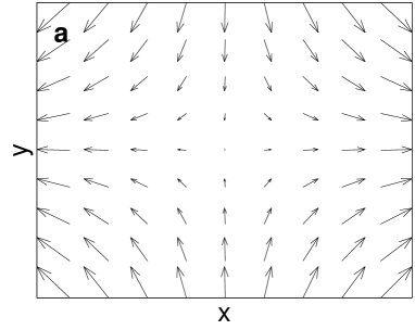
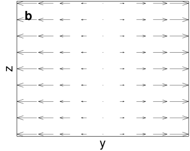
Figure 1: Vectorial plots of the magnetic field (15). a: Intersection for $z=0$. The quadrupolar shape of the field is clearly recognized. b: Intersection for $x=0$ revealing the translational invariance with respect to the $z$-coordinate.

The cut through the $x-y$-plane reveals the quadrupolar shape of the field of the side guide whose translational invariance along the $z$-axis can be easily observed in figure 1b. A corresponding vector potential in the Coulomb gauge is given by

$$\vec{A}=b\left(\begin{array}[]{c}0\\ 0\\ xy\\ \end{array}\right)$$ (19)

Inserting the expressions (15) and (19) into the Hamiltonian (1) thereby adopting atomic units yields

$$H = \frac{1}{2}\triangle-\frac{1}{\sqrt{x^{2}+y^{2}+z^{2}}}+b\,xyp_{z}+\frac{b^{2}}{2}\,x^{2}y^{2}+\frac{b}{2}\left(x\sigma_{x}-y\sigma_{y}\right)$$ (20)

The first two terms of (20) represent the non-relativistic hydrogen atom. The third term which is linear with respect to $b$ replaces the angular Zeeman term which would occur in a homogeneous field. Here the spatial coordinates in $x$ and $y$ couple with the momentum in $z$ direction. The successive diamagnetic term $\propto b^{2}$ represents an oscillator coupling term confining the electronic motion in the $x$ and $y$ direction except for the axis exit channels. This is reminiscent but also very different to the situation in a homogeneous field, where the diamagnetic interactions in the $x$ and $y$ direction separate and represent pure harmonic oscillators. Finally the fifth term represents the coupling of the electronic spin to the spatial coordinates arises from the interaction of its magnetic moment with the field. We here encounter a linear dependence on the spatial coordinates and the gradient $b$. This term prevents the factorization of the motions in coordinate space and spin space. Finally one should note that the only explicit dependence on the coordinate $z$ is due to the Coulomb term. Without this rotationally invariant interaction the system would be invariant under translations with respect to the $z$-coordinate.

Performing the canonical scaling transformation $\bar{x}=b^{\frac{1}{3}}x$ and $\bar{p}=b^{-\frac{1}{3}}p$ the Hamiltonian (20) becomes

$$H=b^{-\frac{2}{3}}\bar{H}=\frac{1}{2}\vec{{p}}^{\,2}-\frac{\bar{Z}}{\sqrt{{x}^{2}+{y}^{2}+{z}^{2}}}+{x}{y}{p}_{z}+\frac{1}{2}\,{x}^{2}{y}^{2}+\frac{1}{2}\left({x}\sigma_{x}-{y}\sigma_{y}\right)$$ (21)

with $\bar{Z}=b^{-\frac{1}{3}}$ and where we have for simplicity omitted the bar on top of the phase space variables. This shows us that employing a scaled energy (scaled Hamiltonian) the only free parameter is the scaled Coulomb coupling strength $\bar{Z}$ that depends on the field gradient. The scaled Hamiltonian describes the motion of an electron in the Coulomb-field of a charge $\bar{Z}$ and the field with gradient $1$. If $b\rightarrow\infty$ the Coulomb term vanishes since $\bar{Z}\rightarrow 0$. In this limit the energy level spacing is expected to scale according to $b^{\frac{2}{3}}$.

III Symmetries and degeneracies in Spin-$\frac{1}{2}$-systems

In this section we analyze the structure of the Hamiltonian (20) in detail. After studying its symmetries we discuss how these symmetries affect the excitation spectrum. As a result of a tedious and elaborate analysis of the Hamiltonian (20) we found 15 distinct symmetry operations leaving it invariant. A complete list is provided in table 1.

$\Sigma_{x}=\sigma_{x}P_{y}P_{z}$	$\Sigma_{y}=P_{x}\sigma_{y}P_{z}$	$\Sigma_{z}=P_{x}P_{y}\sigma_{z}$
$I_{xy}S_{1}^{*}$	$P_{y}P_{z}I_{xy}S_{2}$	$P_{x}P_{y}I_{xy}S_{1}$	$P_{x}P_{z}I_{xy}S_{2}^{*}$
$T\sigma_{x}P_{z}$	$TP_{x}P_{y}P_{z}\sigma_{y}$	$TP_{x}\sigma_{z}$	$TP_{y}$
$TP_{y}I_{xy}S_{1}^{*}$	$TP_{z}I_{xy}S_{2}$	$TP_{x}I_{xy}S_{1}$	$TP_{x}P_{y}P_{z}I_{xy}S_{2}^{*}$

Table 1: Symmetry operations of the Hamiltonian (20). Top part: unitary symmetries. Bottom part: anti-unitary symmetries.

Each symmetry is composed of a number of elementary operations which are shown in table 2.

Operator	Operation	Designation
$P_{x_{i}}$	$x_{i}\rightarrow-x_{i}$	$x_{i}$-parity
$T$	$A\rightarrow A^{*}$	conventional time reversal
$\sigma_{x}$	$\sigma_{y}\rightarrow-\sigma_{y}$ $\sigma_{z}\rightarrow-\sigma_{z}$	Pauli spin matrix x
$\sigma_{y}$	$\sigma_{x}\rightarrow-\sigma_{x}$ $\sigma_{z}\rightarrow-\sigma_{z}$	Pauli spin matrix y
$\sigma_{z}$	$\sigma_{x}\rightarrow-\sigma_{x}$ $\sigma_{y}\rightarrow-\sigma_{y}$	Pauli spin matrix z
$I_{xy}$	$x\rightarrow y$ $y\rightarrow x$  ($\phi\rightarrow-\phi+\frac{\pi}{2}$)	coordinate exchange
$S_{1}=\left(\begin{array}[]{cc}0&1\\ -i&0\\ \end{array}\right)$	$\sigma_{x}\rightarrow-\sigma_{y}$ $\sigma_{y}\rightarrow-\sigma_{x}$ $\sigma_{z}\rightarrow-\sigma_{z}$
$S_{2}=\left(\begin{array}[]{cc}-i&0\\ 0&1\\ \end{array}\right)$	$\sigma_{x}\rightarrow-\sigma_{y}$ $\sigma_{y}\rightarrow\sigma_{x}$ $\sigma_{z}\rightarrow\sigma_{z}$

Table 2: Set of discrete operations out of which all symmetry operations of the Hamiltonian (20) can be composed. Note that $S_{1}$ and $S_{2}$ are given in a basis where $\sigma_{z}$ is diagonal.

All symmetry operations are either unitary or anti-unitary. The anti-unitary ones involve the conventional time reversal operator $T$. In spite of its simplicity our system therefore possesses a wealth of symmetry properties. The algebra of the underlying symmetry group possesses a complicated structure some features of which will be discussed in the following. The operators $\Sigma_{x}$, $\Sigma_{y}$ and $\Sigma_{z}$ generate a sub-group obeying the algebra $\left[\Sigma_{i},\Sigma_{j}\right]=2i\,\epsilon_{ijk}\Sigma_{k}$ reminiscent of angular momentum operators. We have $\Sigma_{i}^{2}=1$. Interestingly these quantities act on both real and spin space. A deeper look into the representation theory of our group reveals a two-fold degeneracy of any energy level similar to those we encountered in our investigations of atoms in a three-dimensional quadrupole trap Lesanovsky04_1 ; Lesanovsky04_2 .

Alternatively this degeneracy can also be established as follows. The operations $\Sigma_{z}$ and $T\sigma_{x}P_{z}$ obey $\left\{\Sigma_{z},T\sigma_{x}P_{z}\right\}=0$. Let $\left|E,\pi\right>$ be an energy eigenstate and at the same time an eigenstate of $\Sigma_{z}$ with

$$\Sigma_{z}\left|E,\pi\right> = \pi\left|E,\pi\right>$$ (22)

and $\pi=\pm 1$. Employing the above anti-commutator one obtains

$$\Sigma_{z}T\sigma_{x}P_{z}\left|E,\pi\right>=-T\sigma_{x}P_{z}\Sigma_{z}\left|E,\pi\right>=-\pi T\sigma_{x}P_{z}\left|E,\pi\right>$$ (23)

The state $T\sigma_{x}P_{z}\left|E,\pi\right>$ can be identified with $\left|E,-\pi\right>$. Hence, as long as $\pi\neq 0$ there is always an orthogonal pair of states possessing the same energy namely $\left|E,\pi\right>$ and $\left|E,-\pi\right>$. We have to emphasize that there occur no further degeneracies in the system. In principle one could think of performing the above calculation repeatedly but now substituting $T\sigma_{x}P_{z}$ with any operator listed in table 1 which anti-commutes with $\Sigma_{z}$. It turns out that all of the resulting states generated by this scheme are either superpositions of $\left|E,\pi\right>$ and $\left|E,-\pi\right>$ or differ only by a phase factor from one of these states.

Out of the 15 symmetry operations one can choose several sets of commuting operators. For the following investigation we choose the set $H$, $\Sigma_{z}$, $P_{y}P_{z}I_{xy}S_{2}$. The combination of $\Sigma_{z}$ and $P_{y}P_{z}I_{xy}S_{2}$ leads to the additional commuting operator $P_{x}P_{z}I_{xy}S_{2}^{*}$. We have found the properties:

$$\left(P_{y}P_{z}I_{xy}S_{2}\right)^{2} = \left(P_{x}P_{z}I_{xy}S_{2}^{*}\right)^{2}=-\Sigma_{z}$$ (24)

$$\left(\Sigma_{z}\right)^{2} = \left(P_{y}P_{z}I_{xy}S_{2}\right)^{4}=\left(P_{x}P_{z}I_{xy}S_{2}^{*}\right)^{4}=1.$$ (25)

For completeness we provide here the general embedding of the above-derived degeneracies due to symmetries. Let us assume we have a general spin-$\frac{1}{2}$-systems with the following accompanying properties:

1. There are two operators $A$ and $B$ commuting with the underlying Hamiltonian: $\left[H,A\right]=\left[H,B\right]=0$.

2. $A$ and $B$ anti-commute: $\left\{A,B\right\}=0$.

3. $A$ is a Hermitian operator. $B$ is an (anti-)unitary operator which can be written as a product $B=RS$ where $R$ and $S$ exclusively act on the real space and the spin space, respectively.

4. The operator $S$ is trace-less: $\text{Tr}\,S=0$.

If these conditions are fullfilled any state is doubly degenerate. This is seen as follows. Property 4 immediately leads to $\text{Tr}\,B=0$. Hence, we find the nonzero eigenvalues of $B$ to appear pairwise with opposite signs. If now $\left|E,b\right>$ is an eigenstate of $B$ and at the same time an energy-eigenstate property 2 implies that

$$BA\left|E,b\right>=-AB\left|E,b\right>=-bA\left|E,b\right>=-b\left|E,-b\right>.$$ (26)

Hence, $\left|E,b\right>$ and $A\left|E,b\right>=\left|E,-b\right>$ are two degenerate energy-eigenstates of the system.

In the present case the two anti-commuting operators are $\Sigma_{z}$ and $T\sigma_{x}P_{z}$. For the case of an atom in a three-dimensional quadrupole field we have $A=J_{z}$ and $B=T\sigma_{x}P_{z}$. In a homogeneous magnetic field the remaining symmetries constitute an Abelian symmetry group leading to exclusively one dimensional irreducible representations i.e. no degeneracies occur. Finally we remark that the reader can find in ref. Haake01 a discussion of degeneracies in spin-$\frac{1}{2}$-systems based on the properties of time-reversal operators.

IV $\Sigma_{z}$-, $P_{y}P_{z}I_{xy}S_{2}$- and $T\sigma_{x}P_{z}$-eigenstates

The operator $P_{y}P_{z}I_{xy}S_{2}$ obeys the eigenvalue relation

$$P_{y}P_{z}I_{xy}S_{2}\left|\kappa\right>=\kappa\left|\kappa\right>.$$ (27)

Since

$$\left|\kappa\right>=\left(P_{y}P_{z}I_{xy}S_{2}\right)^{4}\left|\kappa\right>=\kappa^{4}\left|\kappa\right>$$ (28)

the eigenvalue $\kappa$ can adopt the four values $\pm 1$ and $\pm i$. The reader should note that $P_{y}P_{z}I_{xy}S_{2}$ is a unitary but non-Hermitian operator. We therefore encounter complex eigenvalues. If we apply $\Sigma_{z}$ to the states $\left|\kappa\right>$ we find by exploiting equation (24)

$$\Sigma_{z}\left|\kappa=\pm i\right> = \left|\kappa=\pm i\right>$$ (29)

$$\Sigma_{z}\left|\kappa=\pm 1\right> = -\left|\kappa=\pm 1\right>.$$ (30)

By using the relation $\left(T\sigma_{x}P_{z}\right)\left(P_{y}P_{z}I_{xy}S_{2}\right)-i\left(P_{y}P_{z}I_{xy}S_{2}\right)\left(T\sigma_{x}P_{z}\right)=0$ one finds the degenerate pairs of states in the $P_{y}P_{z}I_{xy}S_{2}$-subspaces: $\left|E,+1\right>$,$\left|E,-i\right>$ and $\left|E,-1\right>$,$\left|E,+i\right>$. Since non-Hermitian operators do not represent physical observables only the quantum number $\pi$ should be of direct relevance for the experimental observation.

We now derive the expectation value of an observable $Y$ in an eigenstate of $\Sigma_{z}$. Assume we have $\left\{Y,\Sigma_{z}\right\}=0$ and hence

$$\left<E,\pi\right|Y\Sigma_{z}\left|E,\pi\right> = -\left<E,\pi\right|\Sigma_{z}Y\left|E,\pi\right>$$ (31)

$$\pi\left<E,\pi\right|Y\left|E,\pi\right> = -\pi\left<E,\pi\right|Y\left|E,\pi\right>.$$ (32)

This immediately leads to the result

$$\left<E,\pi\right|Y\left|E,\pi\right>=0.$$ (33)

The same arguments hold for an observable $Z$ obeying $\left\{Z,P_{y}P_{z}I_{xy}S_{2}\right\}=0$ in which case we obtain

$$\left<E,\kappa\right|Z\left|E,\kappa\right>=0.$$ (34)

In the preceding section we showed the degeneracy of the states $\left|E,\pi\right>$ and $T\sigma_{x}P_{z}\left|E,\pi\right>$. By superimposing these two states eigenstates of the operator $T\sigma_{x}P_{z}$ can be constructed:

$$\left|E,\pm\right>^{T\sigma_{x}P_{z}}=\frac{1}{\sqrt{2}}\left[\left|E,\pi\right>\pm T\sigma_{x}P_{z}\,\left|E,\pi\right>\right].$$ (35)

The corresponding eigenvalue relation is

$$T\sigma_{x}P_{z}\,\left|E,\pm\right>=\pm\left|E,\pm\right>.$$ (36)

V Additional Homogeneous Field in $z$-Direction (Ioffe Field)

The application of an additional homogeneous magnetic field along the $z$-direction (Ioffe field) has a dramatic impact on the properties of the system. In particular the symmetry properties are affected. The Hamiltonian becomes

$$H_{I} = -\frac{1}{2}\triangle_{x,y,z}-\frac{1}{\sqrt{x^{2}+y^{2}+z^{2}}}+b\,xyp_{z}+\frac{b^{2}}{2}\,x^{2}y^{2}+\frac{b}{2}\left(x\sigma_{x}-y\sigma_{y}\right)$$ (37)

$$+\frac{B_{I}}{2}\left(xp_{y}-yp_{x}\right)+\frac{B_{I}^{2}}{8}\left(x^{2}+y^{2}\right)+\frac{B_{I}}{2}\sigma_{z}$$

with $B_{I}$ being the field strength of the Ioffe field. Since both the 2D-quadrupole (due to the side guide) and the magnetic field are perpendicular to each other the homogeneous field terms can simply be added to the Hamiltonian (20). We find the well known Zeeman as well as the diamagnetic oscillator term. The coupling of the spin to the Ioffe field leads to a term being proportional to $\sigma_{z}$. The symmetries of $H_{I}$ are listed in table 3.

$\Sigma_{z}$	$P_{y}P_{z}I_{xy}S_{2}$	$P_{x}P_{z}I_{xy}S_{2}^{*}$
$TP_{x}\sigma_{z}$	$TP_{z}I_{xy}S_{2}$	$TP_{x}P_{y}P_{z}I_{xy}S_{2}^{*}$	$TP_{y}$

Table 3: Symmetries of the Hamiltonian (37), i.e. side guide with Ioffe field. Top line: unitary symmetries. Bottom line: anti-unitary symmetries.

Due to the presence of the additional homogeneous field numerous symmetries are lost (see table 1 for comparison). The remaining operations form a non-Abelian algebra. In contrast to the group operations listed in table 1 there are no two anti-commuting operators. Hence it is not possible to construct pairs of degenerate energy eigenstates as discussed above. Thus, applying the Ioffe field lifts the degeneracies occuring in the absence of it. Even with a finite Ioffe field the operations $\Sigma_{z}$, $P_{y}P_{z}I_{xy}S_{2}$ and $P_{x}P_{z}I_{xy}S_{2}^{*}$ together with $H_{I}$ form a set of commuting operators.

VI Numerical Treatment

In order to obtain many eigenvalues and eigenfunctions of the Hamiltonians (20) and (37) particularly for highly excited Rydberg states we adopt the linear variational principle. Here the bound state solutions of the Schrödinger equation are expanded in a finite set of square integrable basis functions. Determining the expansion coefficients is equivalent to solving a generalized eigenvalue problem in case of non-orthogonal basis functions. The latter is done numerically by employing standard linear algebra techniques and routines.

To accomplish the above we adopt spherical coordinates. The Hamiltonian (20) then becomes

$$H = -\frac{1}{2}\triangle_{r,\theta,\phi}-\frac{1}{r}-ibr\sin\phi\cos\phi\left(\sin^{2}\theta\cos\theta\,r\frac{\partial}{\partial r}-\sin^{3}\theta\frac{\partial}{\partial\theta}\right)$$ (40)

$$+\frac{b^{2}}{2}r^{4}\sin^{4}\theta\sin^{2}\phi\cos^{2}\phi+\frac{b}{2}r\sin\theta\left(\begin{array}[]{cc}0&e^{i\phi}\\ e^{-i\phi}&0\\ \end{array}\right).$$

With an additional Ioffe applied we have to consider the Hamiltonian (37) which reads in spherical coordinates

$$H_{I}=H-i\frac{B_{I}}{2}\frac{\partial}{\partial\phi}+\frac{B_{I}^{2}}{8}r^{2}\sin^{2}\theta+\frac{B_{I}}{2}\sigma_{z}.$$ (41)

We utilize a Sturmian basis set of the form

$$\left|n,l,m,s\right>=R_{n}^{(\zeta,k)}(r)\,Y_{l}^{m}(\theta,\phi)\left|s\right>.$$ (42)

These functions form a complete set in real and spin space but are not orthogonal. The angular part is covered by the well-known spherical harmonics $Y_{l}^{m}(\theta,\phi)$ whereas the two spinor components are addressed by the spin-orbitals $\left|s\right>=\left|\uparrow\right>$ or $\left|\downarrow\right>$. For the radial part we employ

$$R_{n}^{(\zeta,k)}(r)=\sqrt{\frac{n!}{(n+2k)!}}e^{-\frac{\zeta r}{2}}(\zeta r)^{k}L_{n}^{2k}(\zeta r).$$ (43)

with $L_{n}^{2k}(r)$ being the associated Laguerre polynomials. The parameters $k$ and $\zeta$ can be adapted in order to gain an optimal convergence behavior in any spectral region. In particular the non-linear variational parameter $\zeta$ has to adapted such that it corresponds to the inverse of the characteristic length scale of the desired wavefunctions. Similar basis sets have been employed previously by several other authors Clark80 ; Clark82 ; Wunner86 .

The general expansion of an energy eigenstate $\left|E\right>$ in a finite set of basis functions (42) reads

$$\left|E\right>=\sum_{nlms}c_{nlms}\left|n,l,m,s\right>.$$ (44)

From our knowledge of the symmetries of the system we can further specify the appearance of the expansion. In section III we chose $H$, $\Sigma_{z}$ and $P_{y}P_{z}I_{xy}S_{2}$ to be the set of commuting operators whose eigenfunctions we want to construct. We now demand $\left|E\right>$ to be an eigenstate of $P_{y}P_{z}I_{xy}S_{2}$. Exploiting the relations

$$P_{y}P_{z}I_{xy}S_{2}\,Y_{l}^{m}\left|\uparrow\right> = -ie^{-i\frac{\pi}{2}m}(-1)^{l}\,Y_{l}^{m}\left|\uparrow\right>$$ (45)

$$P_{y}P_{z}I_{xy}S_{2}\,Y_{l}^{m}\left|\downarrow\right> = e^{-i\frac{\pi}{2}m}(-1)^{l}\,Y_{l}^{m}\left|\downarrow\right>.$$ (46)

we construct the following expansions for the four $\kappa$-subspaces

$$\left|E,+1\right> = \sum_{nlm}\left[R_{n}(a_{nlm}Y_{2l+1}^{4m+1}+b_{nlm}Y_{2l}^{4m+3})\left|\uparrow\right>+\bar{R}_{n}(c_{nlm}Y_{2l+1}^{4m+2}+d_{nlm}Y_{2l}^{4m+4})\left|\downarrow\right>\right]$$ (47)

$$\left|E,-1\right> = \sum_{nlm}\left[R_{n}(a_{nlm}Y_{2l}^{4m+1}+b_{nlm}Y_{2l+1}^{4m+3})\left|\uparrow\right>+\bar{R}_{n}(c_{nlm}Y_{2l}^{4m+2}+d_{nlm}Y_{2l+1}^{4m+4})\left|\downarrow\right>\right]$$ (48)

$$\left|E,+i\right> = \sum_{nlm}\left[R_{n}(a_{nlm}Y_{2l}^{4m+2}+b_{nlm}Y_{2l+1}^{4m+4})\left|\uparrow\right>+\bar{R}_{n}(c_{nlm}Y_{2l+1}^{4m+1}+d_{nlm}Y_{2l}^{4m+3})\left|\downarrow\right>\right]$$ (49)

$$\left|E,-i\right> = \sum_{nlm}\left[R_{n}(a_{nlm}Y_{2l+1}^{4m+2}+b_{nlm}Y_{2l}^{4m+4})\left|\uparrow\right>+\bar{R}_{n}(c_{nlm}Y_{2l}^{4m+1}+d_{nlm}Y_{2l+1}^{4m+3})\left|\downarrow\right>\right]$$ (50)

The eigenfunctions (47-50) are automatically also eigenfunctions to $\Sigma_{z}$ (see eq. (29) and (30)). Due to the structure of the spherical harmonics $Y_{l}^{m}$ one has to ensure that $\left|m\right|\leq l$. In our calculations the sums run over all valid combinations of $n\leq N$, $l\leq L$ and $m\leq M$ where the maximum indices $N$, $L$ and $M$ can be fixed individually. The expansion becomes exact if $M,N,L\rightarrow\infty$.

Performing the linear variational principle with one of the above expansions leads to a generalized eigenvalue problem $\mathbf{H}\vec{v}=E\mathbf{S}\vec{v}$, where $\mathbf{H}$ and $\mathbf{S}$ are the corresponding matrix representation of the Hamiltonian (40) and the overlap matrix, respectively:

$$\mathbf{H}=\left<E,\kappa\right|H\left|E,\kappa\right> \mathbf{S}=\left<E,\kappa\mid E,\kappa\right>.$$ (51)

The vector $\vec{v}$ contains the expansion coefficients $a_{nlm}$, $b_{nlm}$, $c_{nlm}$ and $d_{nlm}$.

Due to the particular choice of the basis functions (42) the matrices $\mathbf{H}$ and $\mathbf{S}$ become extremely sparse occupied ($\mathbf{S}$ is a penta-banded matrix). In order to solve the generalized eigenvalue equation we utilize the so-called Arnoldi method together with the shift-and-invert method. We adopt routines from the ARPACK package. A more detailed description can be found in Lesanovsky04_2 .

VII Results and Discussion

In this section we analyze our computational results i.e. the eigenvalues and eigenfunctions obtained via the numerical approach described in the previous section. We discuss the spectra and expectation values of several observables as well as the properties of the electronic spin. Furthermore selection rules for electric dipole transitions as well as their strengths are derived. Results for the case of the additional presence of a homogeneous bias field are presented as well.

VII.1 Spectral Properties

With respect to the spectral behavior one can distinguish three regimes: the weak, the intermediate and the strong gradient regime each of which reveals individual characteristics. The appearance of these regimes is not determined by the gradient and the degree of excitation, i.e. energy, but by the scaled energy (see discussion in Sec. I). For simplicity we will refer to the gradient as the relevant quantity characterizing the different regimes. All figures in this subsection show energy levels for manifolds belonging to rather small values for $n$ (typically $(n=5\,-\,7)$) and for large gradients (we cover the range $b=10^{-7}-10^{-4}$) that are not accessible in the laboratory. This was done for reasons of illustration: Our observations and results equally hold for weaker gradients and higher $n$-manifolds (gradients achievable for tight traps on atom chips are of the order of $b=10^{-8}$) which however, due to the high level density, are less suited for a graphical presentation. In the weak gradient regime the spectral behaviour is determined by the linear Zeeman terms. Although the principal quantum number $n$ is not a good quantum number any given level can be assigned to a certain $n$-multiplet. The levels split symmetrically around the zero-field-energy exhibiting the expected linear dependence on $b$. In figure 2a this is exemplarily shown for the $n=5$-multiplet.

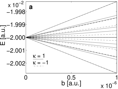
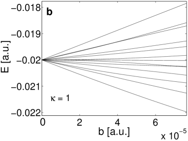
Figure 2: a: Splitting of the energy levels belonging to the $n=5$ multiplet ($\kappa=\pm 1$-subspace) with increasing gradient. The level structure is dominated by the linear Zeeman term. The splitting is linear and symmetric around the energy for $b=0$. b: Intra $n$-manifold mixing of the $n=5$ multiplet in the $\kappa=1$-subspace. Due to the increasing dominance of the diamagnetic term the level splitting becomes non-linear.

The intermediate regime is characterized by the occurence of intra $n$-manifold mixing. Although neighboring $n$-manifolds are still distinguishable the levels now aquire a a nonlinear $b$-dependence which is due to the increasing importance of the diamagnetic term. Sub-levels belonging to different angular momenta mix and thus avoided level-crossings appear. The onset of this intermediate regime scales according to $b\propto n^{-6}$. Figure 2b shows the regime of intermediate gradients of the $n=5$-multiplet. Interestingly we observe here that this nonlinear behaviour in the $l-$mixing regime is very weakly pronounced for the atom in the side guide compared to an atom in a homogeneous magnetic field Friedrich89 . As we enter the strong gradient regime adjacent $n$-manifolds begin to overlap. The spectra are strongly i.e. nonperturbatively influenced by the diamagnetic term. Figure 3 shows this inter $n$-manifold mixing for the $n=6$- and $n=7$-multiplet where the strong coupling leads to large avoided crossings. The mixing threshold scales according to $b\propto n^{-\frac{11}{2}}$ (indicated by the dashed line in figure 3).

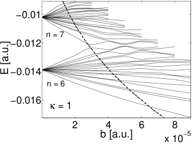
Figure 3: Inter $n$-manifold mixing between the $n=6$- and $n=7$-multiplet in the $\kappa=1$-subspace. The mixing threshold is indicated by the dashed line. A large number of avoided crossings occur.

VII.2 Properties of the Electronic Spin

VII.2.1 $S_{z}$ expectation value

In order to study the mutual influence of coordinate and spin space let us investigate the properties of the electronic spin. The $x$- and $y$-components of the spin operator obey $\left\{\Sigma_{z},S_{x}\right\}=\left\{\Sigma_{z},S_{y}\right\}=0$. Hence using (33) we arrive at

$$\left<S_{x}\right>=\left<S_{y}\right>=0.$$ (52)

Only the expectation value of $S_{z}$ is non-zero in general. This is not obvious since the Hamiltonian (40) does not contain an explicit dependence on $S_{z}$.

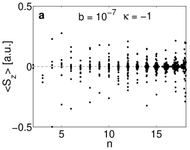
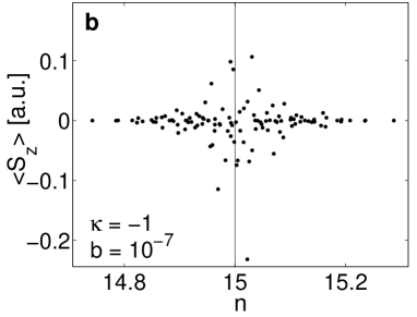
Figure 4: a: Expectation value of the $z$-component of the electronic spin operator for several excited states ($b=10^{-7}$). b: Zoomed view of the $n=15$-multiplet. The magnitude of $\left<S_{z}\right>$ decreases for states possessing a large energy shift due to the external field.

Figure 4a shows the expectation value $\left<S_{z}\right>$ for several excited states as a function of the principal quantum number $n$, which serves as an energetic label. The expectation values are arranged along vertical lines each of which belongs to a certain $n$-multiplet. With increasing degree of excitation these lines widen and begin to overlap as the inter $n$-mixing regime is reached. A zoomed view of the $n=15$-multiplet is shown in figure 4b. We find states experiencing a large energy shift due to the external field thereby possessing a small $S_{z}$ expectation value. For the states shown in this figure $\left<S_{z}\right>$ vanishes for $n>15.2$ and $n<14.8$.

VII.2.2 Spatial Distributions of the Spin Polarization

We now study the relative alignment of the electronic spin and the magnetic field. For a two-component spinor $\left|\Psi\right>=\left(\left|u\right>,\left|d\right>\right)^{T}$ we define

$$W_{SB}(\vec{r}) = \frac{\left<\Psi\mid\vec{r}\right>\left<\vec{r}\right|\vec{S}\vec{B}\left|\vec{r}\right>\left<\vec{r}\mid\Psi\right>}{\left|\vec{S}\right||\vec{B}|\left|\left<\Psi\mid\vec{r}\right>\right|^{2}}=\frac{\left<\Psi\mid\vec{r}\right>(\sigma_{x}\cos\phi-\sigma_{y}\sin\phi)\left<\vec{r}\mid\Psi\right>}{\left|\left<\vec{r}\mid u\right>\right|^{2}+\left|\left<\vec{r}\mid d\right>\right|^{2}}$$ (53)

$$= 2\frac{\text{Re}\left[u^{*}(\vec{r})d(\vec{r})e^{i\phi}\right]}{\left|u(\vec{r})\right|^{2}+\left|d(\vec{r})\right|^{2}}=\left<\cos\gamma\right>\left(\vec{r}\right)$$

$W_{SB}(\vec{r})$ describes the spatial distribution of the spin polarization relative to the local magnetic field. $W_{SB}(\vec{r})=1$ indicates the spin to be oriented parallel to the field whereas we find it antiparallel aligned for $W_{SB}(\vec{r})=-1$. According to (53) $W_{SB}(\vec{r})$ can be interpreted as the local expectation value of the cosine of the angle $\gamma$ between $\vec{S}$ and $\vec{B}$. Since in a homogenous field the projection of the spin onto the field direction is conserved $W_{SB}(\vec{r})$ would be either $+1$ or $-1$ throughout the whole space. In the field of the side guide, however, we expect a much richer structure resulting from the coupling of the coordinate and the spin degrees of freedom.

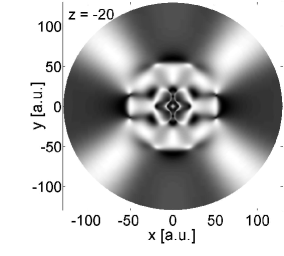
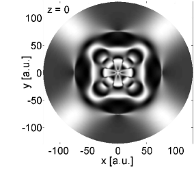
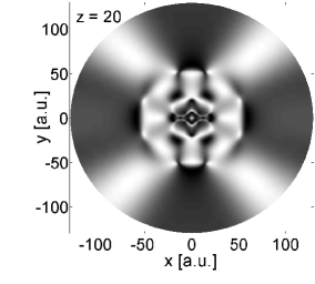
Figure 5: Tomographic cuts through the spin polarization $W_{SB}$ of the $83$rd excited state. The state belongs to the $n=8$ multiplet within the $\kappa=1$-subspace ($b=10^{-7}$). The cuts are made at $z=\pm 20$ and $z=0$. Positive and negative values are indicated white and black, respectively. We observe a rich pattern of different spin polarizations around the origin. From $r\approx 60$ on the nodal structure is replaced by a regular striped pattern varying periodically with the azimuthal angle $\phi$.

Figure 5 shows three tomographic cuts of a the spin polarization $W_{SB}$ of the $83rd$ excited state in the $\kappa=1$-subspace. In the vicinity of the coordinate center we observe a large number of nodes. From $\rho\approx 60$ on the complex nodal structure is replaced by a smooth regular pattern exhibiting a periodicity with respect to the azimuthal angle $\phi$. Here $W_{SB}(\vec{r})$ becomes almost independent of the $z$-coordinate. This feature seems to be induced mainly by the magnetic interaction which is invariant under translations along $z$. One identifies four sectors reminiscent of the quadrupolar structure of the magnetic field of the guides. In the present case we apparently have a anti-parallel alignment in the $x=0$- and $y=0$-plane and a parallel one between these planes. The densities are invariant under the operations $P_{x}P_{y}$ and $P_{z}I_{xy}$ which are equivalent to $\Sigma_{z}$ and $P_{y}P_{z}I_{xy}S_{2}$ when acting on real and scalar quantities.

VII.3 Electric Dipole Transitions

We now consider electromagnetic transitions between electronic states in the framework of the dipole approximation. The transition amplitude between the initial state $\left|i\right>$ and the final state $\left|f\right>$ is then given by the squared modulus of the matrix element $\left<i\right|D\left|f\right>$. In the length gauge $D$ takes the forms $D_{\sigma^{\pm}}=\frac{1}{\sqrt{2}}\left(x\pm iy\right)=\frac{1}{\sqrt{2}}r\sin\theta e^{\pm i\phi}$ and $D_{\pi}=z=r\cos\theta$ for $\sigma^{\pm}$- and $\pi$-transitions, respectively.

Exploiting the symmetry properties of the $P_{y}P_{z}I_{xy}S_{2}$-eigenstates yields

$$\left<E,\kappa\right|\left(P_{y}P_{z}I_{xy}S_{2}\right)^{+}z\,P_{y}P_{z}I_{xy}S_{2}\left|E^{\prime},\kappa^{\prime}\right>=\kappa^{*}\kappa^{\prime}\left<E,\kappa\right|z\left|E^{\prime},\kappa^{\prime}\right>=-\left<E,\kappa\right|z\left|E^{\prime},\kappa^{\prime}\right>$$ (54)

which leads to the expression

$$\left(\kappa^{*}\kappa^{\prime}+1\right)\left<E,\kappa\right|z\left|E^{\prime},\kappa^{\prime}\right>=0.$$ (55)

Here we have used $\left<E,\kappa\right|\left(P_{y}P_{z}I_{xy}S_{2}\right)^{+}=\left<\kappa\right|\kappa^{*}$. Apparently the matrix element for $\pi$-transitions can only be non-zero for the following combinations of $\kappa$ and $\kappa^{\prime}$:

$$\pi:\quad(\kappa,\kappa^{\prime})=(1,-1),(-1,1),(i,-i),(-i,i)$$ (56)

The above shows also that the expectation value of the $z-$coordinate vanishes for any eigenstate i.e. we have $\left<E,\kappa|z|E,\kappa\right>=0$ For $\sigma^{\pm}$-transition one obtains in a similar way

$$\sigma^{+}:\quad(\kappa,\kappa^{\prime}) = (i,1),(1,-i),(-1,i),(-i,-1)$$ (57)

$$\sigma^{-}:\quad(\kappa,\kappa^{\prime}) = (-i,1),(1,i),(-1,-i),(i,-1).$$ (58)

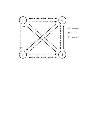
Figure 6: Graphical representation of allowed dipole transitions between $\kappa$-subspaces. The arrows point from $\kappa$ to $\kappa^{\prime}$.

Figure 6 presents an overview of the allowed dipole transitions between the $\kappa$-subspaces.

We have calculated the dipole strengths for transitions from the ground state to excited states.

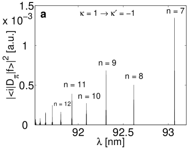
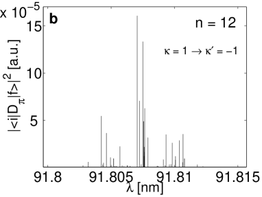
Figure 7: a: Dipole strenghts for $\pi$-transition from the ground state of the $\kappa=1$-subspace to excited states belonging to the $\kappa=-1$-subspace ($b=10^{-7}$). The line for smallest $\lambda$ belongs to the $n=1\rightarrow 7$-transition. b: Zoomed view of the line belonging to the transition to the $n=12$-multiplet. The line center is dominated by two sub-lines. The two bunches accompanying the line center at its left and right hand side possess a much smaller dipole strength.

Figure 7 shows the results we obtain for $\pi$-transitions between the $\kappa=1$- and $\kappa^{\prime}=-1$-subspace. In figure 7a we observe a general decrease of the dipole strengths with decreasing transition wavelengths. However, the decrease is not monotonous as it would be in the case of a homogeneous or a 3D-quadrupole field Lesanovsky04_2 . One rather finds a modulation on top of the transition amplitudes where the $n=8$-, $n=10$- and $n=12$-multiplet exhibit smaller dipole strengths than both of their neighbors. Figure 7b shows a zoomed view of the $n=1\rightarrow 12$ transition line. Its structure is dominated by two sub-lines located in the line center. The central bunch is almost symmetrically accompanied by two bunches of sub-lines located for smaller and larger wavelength, respectively.

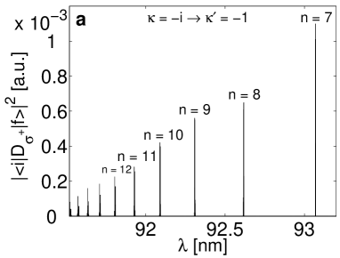
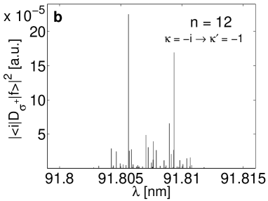
Figure 8: a: Dipole strenghts for $\sigma^{+}$-transition from the ground state of the $\kappa=-i$-subspace to excited states belonging to the $\kappa=-1$-subspace ($b=10^{-7}$). The line for smallest $\lambda$ belongs to the $n=1\rightarrow 7$-transition. b: Zoomed view of the line belonging to the transition to the $n=12$-multiplet. The line consists of three bunches each of which consisting of a number of sub-lines. The line is dominated by two sub-lines one of each located in the left and right hand side bunch.

For $\sigma^{+}$-transitions the dipole strengths are systematically decreasing with decreasing wavelength (figure 8a). In the zoomed view (figure 8b) we also notice the structure consisting of three bunches of sub-lines. Again there are two dominating lines which are now located in the two outer bunches rather than in the central one.

VII.4 Magnetic Guide with a Ioffe field

As discussed in section II an additionally applied homogeneous field leads to severe changes of the symmetry properties of the atomic system. Apart from the lifting of the degeneracies also a significant influence on the electronic spin and the transition amplitudes have to be expected.

Apparently there has to be a critical radius $\rho_{c}$ at which both fields are equal in strength. For a given gradient $b$ and homogeneous field strength $B_{I}$ it is given by $\rho_{c}=\frac{B_{I}}{b}$. Taking into account the scaling $\left<\rho\right>\propto n^{2}$ we expect states with

$$n_{c}=\sqrt{\frac{B_{I}}{b}}$$ (59)

to be equally affected by both fields. Hence, the states having $n\ll n_{c}$ or $n\gg n_{c}$ should be dominated by the homogeneous field or the field of the side guide, respectively.

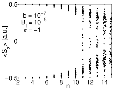
Figure 9: Expectation values of the $z$-component of the electronic spin at a finite homogeneous field strength ($B_{I}=10^{-5}$) and a gradient of $b=10^{-7}$. At low degree of excitation the homogeneous field dominates the electronic states. At this regime $S_{z}$ becomes an approximate constant of motion admitting $\left<S_{z}\right>$ to possess one of the two possible values $\pm\frac{1}{2}$. States lying above the critical principal quantum number $n_{c}$ become increasingly dominated by the quadrupole field. As a result the expecation values tend towards $\left<S_{z}\right>=0$.

Figure 9 shows the expectation values of $S_{z}$ for a gradient $b=10^{-7}$ and a homogeneous field strength $B_{I}=10^{-5}$. This yields the critical principal quantum number $n_{c}=10$. Indeed one finds for $n\ll 10$ the expected dominance of the homogeneous field. In this regime $\left<S_{z}\right>$ is approximately allowed to possess one of the two values $\pm\frac{1}{2}$. This is due to the fact that $S_{z}$ becomes an approximate constant of motion. For $n>10$ we observe the expectation values to move towards zero which is expected from the results shown in figure 4. We have to remark that since the symmetry $\Sigma_{z}$ persists the expectation values of $S_{x}$ and $S_{y}$ vanish even for finite strength of the homogeneous field.

Apart from the spin expectation value also the spin polarization exhibits significant changes if a Ioffe field is switched on. For a sufficient high field strength or low degree of excitation $(n<n_{c})$, respectively, the structure of the electronic states is dominated by the Ioffe field. Here the spin is expected to be aligned with the homogeneous field. Since $W_{SB}$ describes the projection of the electronic spin onto the direction of the side guide field which is perpendicular to the Ioffe field one expects $W_{SB}$ to be approximately zero in this regime.

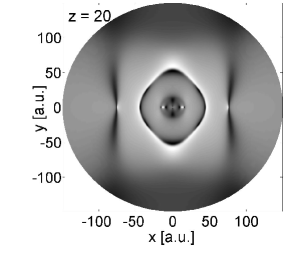
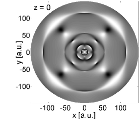
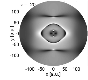
Figure 10: Tomographic cuts through the spin polarization $W_{SB}$ (equation (53)) of the $83$rd excited state at a finite Ioffe field strength $B_{I}=10^{-5}$. The state belongs to the $n=8$ multiplet inside the $\kappa=1$-subspace ($b=10^{-7}$). The cuts are made at $z=\pm 20$ and $z=0$. Positive and negative values are indicated by white and black, respectively. One observes large gray regions with $W_{SB}\approx 0$.

Figure 10 illustrates the $SB$ polarization $W_{SB}$ (equation (53)) for the state shown in figure 5 but for a Ioffe field strength $B_{I}=10^{-5}$. The state is located inside the $n=8$ multiplet which lies below the critical quantum number $n_{c}=10$. Thus the states structure is dominated by the Ioffe field. As expected from the discussion above we observe large gray regions indicating $W_{SB}=0$. The geometry of the side guide field is barely recognized for the cut made at $z=0$. Unlike in figure 5 there are only small regions exhibiting a well-defined spin orientation that is dominated by the side guide, i.e either $W_{SB}=-1$ or $W_{SB}=1$.

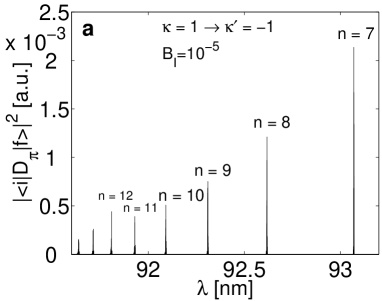
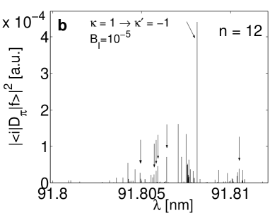
Figure 11: a: Dipole strengths for $\pi$-transition from the ground state of the $\kappa=1$-subspace to excited states belonging to the $\kappa=-1$-subspace ($b=10^{-7}$ and $B_{I}=10^{-5}$). The line for smallest $\lambda$ belongs to the $n=1\rightarrow 7$-transition. b: Zoomed view of the line belonging to the transition to the $n=12$-multiplet. Several additional lines appear at finite homogeneous field strength (some are marked by an arrow). The line center is dominated by a single sub-line emerging from a transition which is induced by the external homogeneous field.

Figure 11a shows the dipole strengths for $\pi$-transitions from the ground state in the $\kappa=1$-subspace to various states in the $\kappa=-1$-subspace. Compared to the $B_{I}=0$ case the dipole strengths are increased by approximately $70\%$. The transition strengths increase with increasing transition wavelengths. Again there seems to occur some kind of modulation as already seen in figure 7a but being less pronounced here. In the present case the $n=12$-transition exhibits a larger transition amplitude than its neighbors. In figure 11b we show a zoomed view of the line belonging to the $n=12$-transition. Due to the presence of the homogeneous field a number of additional lines appear some of which are marked by an arrow. In contrast to the $B_{I}=0$ case the $n=12$ line is dominated by a single sub-line originating from a transition induced by the presence of the homogeneous field.

VIII Conclusion and Outlook

We have studied electronically excited hydrogen atoms located in a magnetic guide. Including pseudo-potentials Gonzales03 for the atomic core could be straight forwardly extended to describe e.g. alkali atoms. The magnetic guide represents a microtrap used to confine ultracold atomic systems. The motion of the valence electron has been described by an effective one-body approach. Both the coupling of the spatial degrees of freedom (para- and diamagnetism) as well as the spin degrees of freedom to the external field have been taken into account. The linear variational principle has been used to solve the stationary Schrödinger equation: Employing a Sturmian basis set enabled us to converge a large number of eigenfunctions.

A careful inspection of the Hamiltonian yields an amazingly large number of symmetries involving both the spin and spatial degrees of freedom: We have found 15 symmetry operations of both unitary and anti-unitary character. This allows for a classification of the electronic eigenstates with respect to a complete set of commuting constants of motion. The latter involve the Hermitian $\Sigma_{z}$-operator which is a combined spin and parity operator and the unitary but non-Hermitian operator $P_{y}P_{z}I_{xy}S_{2}$ which involves parity and permutation operators. Employing specific anticommuting operators of this symmetry group we could prove the two-fold degeneracy of each energy level. This feature is indeed shown to be generic for spin-$\frac{1}{2}$-systems exhibiting certain symmetry properties. We have discussed how the symmetries are affected if an additional homogeneous magnetic field is applied in order to obtain a Ioffe-Pritchard type trap. In this case only $7$ symmetry operations remain including $\Sigma_{z}$, $P_{y}P_{z}I_{xy}S_{2}$ and $P_{x}P_{z}I_{xy}S_{2}^{*}$.

Spectra have been investigated up to energies corresponding to a principal quantum number of $n\approx 15$. In the low gradient regime degenerate $n$-manifolds split up symmetrically around the zero field energy. For the intra-$n$-mixing regime only a very weak restructuring takes place inside any $n$-multiplet i.e. we observe only a minor nonlinear behaviour of the energies on the gradient. For even higher gradients the inter-$n$-mixing takes place where states belonging to adjacent multiplets begin to mix and avoided crossings dominate the spectrum. Scaling relations for both, the inter- and the intra-$n$-mixing have been provided.

Effects due to the coupling of the spin and spatial degrees of freedom have been studied in detail. An analysis of the spin-field orientation has been performed by utilizing the distribution of the spin polarization. For electronic states in the magnetic guide $W_{SB}$ reveals a rich nodal and island structure which is absent for an atom in a uniform field. Moreover an analysis of the $S_{z}$ expectation value has been performed. It has been shown that states being energetically strongly affected by the presence of the magnetic guide possess a small expectation value of $S_{z}$.

We have derived selection rules for the quantum number $\kappa$ belonging to the $P_{y}P_{z}I_{xy}S_{2}$ symmetry operator for linear as well as circular polarized dipole transitions. Wave lengths and dipole strengths from the ground to Rydberg states were analyzed. In particular for $\pi$ transitions we have found a global modulation of the transition amplitudes. The impact of the presence of an additional homogeneous magnetic field (along the wire involved in the set-up of the side guide) on several relevant quantities has been studied. This includes the $S_{z}$-expectation values and the electric dipole transition amplitudes.

Let us now comment on the approach chosen in the present work. Neglecting the fine and hyperfine structure of the atom as well as omitting the influence of the core scattering events represent, at least for certain species and regimes (high excitations !), certainly a good approximation to the true physical system. Another approximation is the fact that we centered the nucleus at the minimum of the field configuration. This is suggested by our assumption that we have ultracold atoms with an extremely small kinetic c.m. energy in tight traps leading to a well-localized atomic c.m. Nevertheless, it is expected that the c.m. motion blurs the effects ocurring for an atom with a fixed nucleus. Beyond this, it is well-known that already in the presence of a homogeneous magnetic field the c.m. and electronic motions of atoms do not separate i.e. they perform an intimately coupled motion Avron78 ; Johnson83 ; Schmelcher94 ; Schmelcher92 ; Dippel94 . Then the immediate question arises how this coupling might look like in our inhomogeneous field configuration and in particular what its impact on the overall electronic motion is. To investigate this is a challenging task which needs careful consideration and clearly goes beyond the scope of the present work.

IX Acknowledgments

We are most thankful to Ofir Alon for fruitful discussions regarding the group theoretical aspects of the present work. I.L. acknowledges a scholarship by the Landesgraduiertenförderungsgesetz of the state of Baden-Württemberg.

References

- (1) R. Folman et al, Adv. At. Mol. Opt. Phys. 48, 263 (2002)
- (2) H. Friedrich and D. Wintgen, Phys. Rep. 183, 37 (1989)
- (3) H. Ruder et al, Atoms in Strong Magnetic Fields, Springer 1992
- (4) H. Friedrich and B. Eckhardt (eds.), Classical, Semiclassical and Quantum Dynamics in Atoms, Lecture Notes in Physics 485, Springer Verlag Heidelberg 1997
- (5) Atoms and Molecules in Strong External Fields, ed. by P. Schmelcher and W. Schweizer, Plenum Press 1998
- (6) Atoms and Molecules in Intense Fields, Eds. L.S. Cederbaum, K.C. Kulander and N.H. March, Springer Series: Structure and Bonding 86, 27 (1997)
- (7) T.H. Bergeman et al, J. Opt. Soc. Am. B 6, 2249 (1989)
- (8) K. Berg-Sorensen, M.M. Burns, J.A. Golovchenko and L.V. Hau, Phys. Rev. A 53, 1653 (1996)
- (9) J.P. Burke, C.H. Greene and B.D. Esry, Phys. Rev. A 54, 3225 (1996)
- (10) C.V. Sukumar and D.M. Brink, Phys. Rev. A 56, 2451 (1997)
- (11) E.A. Hinds and C. Eberlein, Phys. Rev. A 61, 033614 (2000)
- (12) R.M. Potvliege and V. Zehnle, Phys. Rev. A 63, 025601 (2001)
- (13) I. Lesanovsky, J. Schmiedmayer and P. Schmelcher, Europhys. Lett. 65, 478 (2004)
- (14) C. W. Clark and K. T. Taylor, J. Phys. B: At. Mol. Phys 13, L737-L743 (1980)
- (15) C. W. Clark and K. T. Taylor, J. Phys. B: At. Mol. Phys 15, 1175-1193 (1982)
- (16) G. Wunner, M. Kost, and H. Ruder, Phys. Rev. A 33, 1444 (1986)
- (17) I. Lesanovsky, J. Schmiedmayer and P. Schmelcher, Phys. Rev. A 69, 053405 (2004)
- (18) F. Haake, Quantum Signatures of Chaos, Springer (2001)
- (19) R. Gonzáles-Férez and P. Schmelcher, Eur. Phys. J. D 23, 189-199 (2003)
- (20) J. E. Avron, I. W. Herbst and B. Simon, Ann. Phys. (N.Y.) 114, 431 (1978)
- (21) B. R. Johnson, J. O. Hirschfelder and K. H. Yang, Rev. Mod. Physics 55, 109 (1983)
- (22) P. Schmelcher, L. S. Cederbaum an U. Kappes, Conceptual Trends in Quantum Chemistry, p. 1-51 (1994), Eds. E. S. Kryachko and J. L. Calais, Kluwer Academic Publishers
- (23) P. Schmelcher and L. S. Cederbaum, Phys.Lett. A 164, 305 (1992)
- (24) O. Dippel, P. Schmelcher and L. S. Cederbaum, Phys. Rev. A 49, 4415 (1994)