On the recombination in high-order harmonic generation in molecules

Abstract

We show that the dependence of high-order harmonic generation (HHG) on the molecular orientation can be understood within a theoretical treatment that does not involve the strong field of the laser. The results for H₂ show excellent agreement with time-dependent strong field calculations for model molecules, and this motivates a prediction for the orientation dependence of HHG from the N₂ 3$\sigma_{g}$ valence orbital. For both molecules, we find that the polarization of recombination photons is influenced by the molecular orientation. The variations are particularly pronounced for the N₂ valence orbital, which can be explained by the presence of atomic p-orbitals.

I Introduction

In this paper we establish a connection between photoionization/recombination (weak field processes) and high-order harmonic generation (a non-linear phenomenon in strong-field physics). The latter process is one of the most studied aspects of intense-laser physics because it serves as a source of coherent radiation at high frequencies krausz01 ; hentschel01 . High-order harmonic generation can be explained by a recollision mechanism corkum93 : Close to the maximum of the electric field of a femtosecond optical laser pulse a molecule is ionized. A free electron wave packet enters the continuum and follows the electric field of the laser. If the laser is linearly polarized the electron will approach the molecule again. The most energetic recollisions take place near the second zero of the laser electric field after electron release corkum93 . Hence, the laser field at the time of recollision can be considered as small. The optical laser drives the electronic wave packet far away from the molecule (as compared to the size of the molecule). Due to rapid wave packet spreading the electronic wave packet will recollide approximately as a plane wave with its momentum parallel to the laser polarization. Possible consequences of recollision are recombination, elastic scattering or double ionization. In the recombination process a photon is emitted, preferably parallel to the beam axis of the incident laser and with a frequency that is a multiple of the incident laser frequency, therefore called high harmonic. By appropriate superposition of different harmonics one can create attosecond pulses which may be utilized to probe fast atomic and molecular processes krausz01 . If the return time of the electronic wave packet is well defined one can even think of using HHG itself as a probe for time-dependent processes. The ionization by the laser would represent the pump pulse and the recolliding wave packet would represent the probe pulse. The time between those two events is shorter than an optical cycle of the laser. This may open the door to the time-resolved investigation of very fast atomic and molecular processes, cf. also the method described in Ref. niikura03 .

In recent years there has been growing interest in HHG from molecules. The dependence on molecular orientation has been studied experimentally hhgexp and theoretically hhgtheo . Considering the complexity of this process, theoretical investigations have been carried out mostly for H₂ and H${}_{2}^{+}$ until now. How to overcome this? As indicated above, at the time of recollision, when the radiative recombination occurs, the electric field of the laser can be considered to be small for the highest harmonics. In the following we will use an approximation in which the influence of the laser field on the recombination is considered to be even negligible so that the computational methods developed in the context of photoionization can be used. Although this will not cover all the dynamics of HHG, it should explain quite well dependencies of the high harmonics on the molecular geometry and orientation. As we will show, this is indeed the case. As a consequence it will be possible to describe HHG in much more complicated targets in the future by shifting the focus from the exact treatment of the time evolution towards the exact treatment of the final molecular interaction, the recombination in high-order harmonic generation.

II Method

In the recombination process the electron approaches the molecular core and a photon is ejected, leaving the molecule predominantly in its ground state. The dynamics of this process is contained in its transition amplitude. Since recombination is (microscopically) time reversed photoionization one can use as recombination transition amplitudes the complex conjugated photoionization transition amplitudes. Furthermore, since we are here not interested in near threshold behavior we can calculate those photoionization transition amplitudes easily using the frozen core Hartree Fock (FCHF) method : The molecular ground state wave function is derived in a self-consistent-field approximation. The state of the ionized molecule is then obtained by removing one electronic charge out of the orbital that is ionized. The molecule is not allowed to relax (’frozen core’). The photoelectron orbitals were obtained using an iterative procedure to solve the Lippmann-Schwinger equation associated with the one-electron Schrödinger equation that these orbitals satisfy (for further details see lucchese82 ).

For the mathematical description of the process the density matrix formalism blum81 has been applied (see also bzdr ; lohmann ). To be able do so we must model the recombination process. We know the ground states of the neutral molecule and of the singly charged molecular core, $\left|\Lambda_{0}\right\rangle$ and $\left|\Lambda_{c}\right\rangle$, respectively. We assume that the molecular orientation ${\rm\bf m}$ does not change during the process. We also know the state $\left|{\rm\bf k}^{(+)}_{e}\right\rangle$ of the incident electron. (In the following we will sum over not resolved molecular vibrational states and not resolved spin polarization states of the electron.) Naturally, the photon, with a frequency $\omega_{p}$, will be polarized. Therefore the full density matrix $\rho$ of the state after recombination in dipole approximation reads

$$\rho = \left|{\rm\bf m}\,\Lambda_{0}\,\bm{\varepsilon}\,\omega_{p}\right\rangle\left\langle{\rm\bf m}\,\Lambda_{0}\,\bm{\varepsilon}\,\omega_{p}\right|$$ (1)

$$= T\left|{\rm\bf m}\,\Lambda_{c}\,{\rm\bf k}^{(+)}_{e}\right\rangle\left\langle{\rm\bf m}\,\Lambda_{c}\,{\rm\bf k}^{(+)}_{e}\right|T^{+},$$

where $\bm{\varepsilon}$ is the polarization vector of the photon and T the transition operator, i.e., the dipole operator. The photon properties will be measured in a detector in a direction ${\rm\bf n}_{p}$. For a perfect detector one gets by projecting on the different polarization states, which are $\left|\lambda\right\rangle\epsilon\{\left|-1\right\rangle,\left|0\right\rangle,\left|1\right\rangle\}$ in an arbitrary reference frame, for the matrix elements $\rho(\lambda,\lambda^{\prime})$ of the density matrix $\rho$

$$\rho(\lambda,\lambda^{\prime})=\left\langle{\rm\bf m}\,\Lambda_{0}\,{\rm\bf n}_{p}\lambda\,\omega_{p}\right|\rho\left|{\rm\bf m}\,\Lambda_{0}\,{\rm\bf n}_{p}\,\lambda^{\prime}\,\omega_{p}\right\rangle.$$ (2)

A common description of photon polarization employs the Stokes parameters. The Stokes parameters are defined in a reference frame which z-axis is parallel to the photon momentum blum81 . In this frame the right (left) circularly polarized photon state is $\left|+1\right\rangle$ ($\left|-1\right\rangle$). ($\left|0\right\rangle$ does not exist in this reference frame due to the transversal nature of the light.) The four Stokes parameters are : the total intensity $I$, the degree of circular polarization $p_{3}=(I_{+1}-I_{-1})/I$ and the two degrees of linear polarization $p_{1}=(I(0^{\rm o})-I(90^{\rm o}))/I$ and $p_{2}=(I(45^{\rm o})-I(135^{\rm o}))/I$. ($\varphi$ in $I(\varphi)$ starts at the x-axis in the xy-plane.) In the reference frame of the Stokes parameters one gets

$$I = \rho(1,1)+\rho(-1,-1)$$ (3a)

$$p_{3} = \left(\rho(1,1)-\rho(-1,-1)\right)\cdot I^{-1}$$ (3b)

$$p_{1} = -\left(\rho(1,-1)+\rho(-1,1)\right)\cdot I^{-1}$$ (3c)

$$p_{2} = -i\,\left(\rho(1,-1)-\rho(-1,1)\right)\cdot I^{-1}.$$ (3d)

The electronic wave function $\left|{\rm\bf k}^{(+)}_{e}\right\rangle$ can be expanded into spherical harmonics dill76 . However, due to the non-spherical molecular potential the dipole selection rules do not restrict the expansion as in atoms. Nevertheless, both, bound and continuum electron wave functions converge quite rapidly. Therefore, to a very good approximation a limited number of terms is sufficient, truncating the expansion at a certain $l_{max}$. $\rho(\lambda,\lambda^{\prime})$ can be split into a kinematical and a geometrical part

$$\rho(\lambda,\lambda^{\prime})=\sum_{\Gamma=0}^{2}\sum_{{\cal L}=0}^{2\,l_{\rm max}}\sum_{d=|\Gamma-{\cal L}|}^{\Gamma+{\cal L}}M_{d{\cal L}\Gamma}\sum_{\gamma=-\Gamma}^{\Gamma}(-)^{1-\lambda^{\prime}}\left(1\lambda,1-\lambda^{\prime}|\Gamma\gamma\right)\,Y^{d{\cal L}}_{\Gamma-\gamma}\left({\rm\bf m},{\rm\bf k}^{0}_{e}\right).$$ (4)

where $(.,.|.)$ are Clebsch-Gordan coefficients. In Equ. 4 we have used $l_{max}=10$. The geometrical dependencies are expressed in bipolar spherical harmonics,

$$Y^{d{\cal L}}_{\Gamma-\gamma}\left({\rm\bf m},{\rm\bf k}^{0}_{e}\right)=\sum_{\delta=-d}^{d}\sum_{{\cal M}=-{\cal L}}^{\cal L}\left(d\delta,{\cal L}{\cal M}|\Gamma-\gamma\right)\,Y_{d\delta}\left({\rm\bf m}\right)\,Y_{{\cal L}{\cal M}}\left({\rm\bf k}^{0}_{e}\right),$$ (5)

with spherical harmonics $Y_{kq}$ and ${\rm\bf k}^{0}_{e}$ as the normalized electron momentum. The reference frame is given through the photon. The dynamical coefficient is

$$M_{d{\cal L}\Gamma} = \hat{d}\,\hat{\cal L}\sum_{l=0}^{l_{\rm max}}\sum_{m_{m}=-(\Lambda^{0}+1)}^{\Lambda^{0}+1}\sum_{\lambda_{m}=-1}^{1}\sum_{l^{\prime}=0}^{l_{\rm max}}\sum_{m^{\prime}_{m}=-(\Lambda^{0}+1)}^{\Lambda^{0}+1}\sum_{\lambda^{\prime}_{m}=-1}^{1}(-)^{1+m_{m}+\lambda^{\prime}_{m}+\Gamma}\,\hat{l}\,\hat{l}^{\prime}\,R_{lm_{m}\lambda_{m}}\,R_{l^{\prime}m^{\prime}_{m}\lambda^{\prime}_{m}}^{*}$$ (14)

$$\times\left(\begin{array}[]{ccc}l&l^{\prime}&\cal L\\ 0&0&0\end{array}\right)\left(\begin{array}[]{ccc}l&l^{\prime}&\cal L\\ -m_{m}&m^{\prime}_{m}&\alpha_{m}\end{array}\right)\left(\begin{array}[]{ccc}1&1&\Gamma\\ \lambda_{m}&-\lambda^{\prime}_{m}&-\alpha_{m}\end{array}\right)\left(\begin{array}[]{ccc}\cal L&\Gamma&d\\ \alpha_{m}&-\alpha_{m}&0\end{array}\right),$$

where $\Lambda^{0}$ is $0$ if the recombined orbital has $\sigma$ symmetry and $1$ if it has $\pi$ symmetry. In Eq. (14) Wigner 3J symbols have been used. A hat over a quantum number means $\hat{l}=\sqrt{2l+1}$. The dynamical part is calculated in the molecular body frame (symbolized by a sub-index $m$ at the quantum numbers). By applying microscopic time reversal, the recombination matrix element in the molecular body frame in length form is

$$R_{lm_{m}\lambda_{m}}\equiv\omega_{p}\left(i^{-l}\,\exp\left(i\Delta_{l}\right)\left\langle\Lambda_{c}\,lm_{m}\right|d_{\lambda_{m}}\left|\Lambda_{0}\lambda_{m}\right\rangle\right)^{*},$$ (15)

where $\omega_{p}$ is the energy of the photon, $\Delta_{l}$ is the Coulomb phase shift, and $\left\langle\Lambda_{c}\,lm_{m}\right|d_{\lambda_{m}}\left|\Lambda_{0}\lambda_{m}\right\rangle$ is the photoionization dipole matrix element in the body frame with the dipole operator $d_{\lambda_{m}}$.

III Results for H₂

Using the formulae of the last section one can calculate the photon intensity and polarization, the Stokes parameters, as a function of the electron energy and for different orientations of the molecule and electron and photon propagation directions. Here we will focus on the HHG geometry (see Fig. 1), where the electron momentum is perpendicular to the emission direction of the photon. In the following, we distinguish between two cases: (I) the molecule lies in the plane spanned by the electron momentum and the photon direction, and (II) the molecule rotates in the plane perpendicular to the photon direction. We have first calculated the intensity for H₂ recombination in geometry (I) as a function of the molecular orientation. Here, the photon is polarized parallel to the electron momentum for symmetry reasons. The calculation was carried out for different bond lengths and for different wavelengths of the electron (see Fig. 2). One finds a pronounced minimum, which shifts if one changes the bond length of the molecule or if one changes the wavelength of the electron.

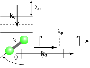
Figure 1: The recombination geometry is shown schematically. The molecule with a bond length $r_{0}$ is oriented relative to the electron momentum ${\rm\bf k}_{e}$ under an angle $\theta$. The photon is emitted perpendicular to the electron momentum.

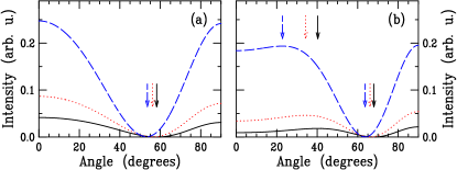
Figure 2: Dependence of the recombination photon intensity on the angle between molecular orientation and the electron momentum for H₂. The molecule lies in the plane spanned by electron momentum and photon direction [geometry (I)]. The solid curves are for an electron wavelength $\lambda_{e}$ of $1.4\,\,\rm{a.u.}$, the dotted curves for $\lambda_{e}=1.6\,\,\rm{a.u.}$ and the dashed curves for $\lambda_{e}=1.8\,\,\rm{a.u.}$ (a) Molecular bond length $r_{0}=1.4\,\,\rm{a.u.}$; (b) $r_{0}=2.0\,\,\rm{a.u.}$. The positions of minima and maxima are marked by arrows. Obviously, the positions of the extrema depend on the bond length and on the wavelength of the electron. This behavior can be explained by a two-center interference model (see text). Clearly, the minima are very pronounced.

One can explain the general behavior at electron wavelengths comparable to the bond length of the molecule by the well-known two-center interference. Here one imagines the diatomic molecule as two centers which are hit coherently by the same plane electron wave, but with a phase difference that depends on the molecular orientation towards the electron. Recombination leads to the ejection of a photon. Interference occurs, since it is not known which center has emitted the photon. Changing the electron wavelength and/or the molecular orientation will alter the phase difference so that an interference pattern will be obtained. At the energies used here, the photon wavelength is much larger than the dimension of the molecule, so that one can neglect the phase shift resulting from the orientation of the molecule with respect to the photon. The bond length $r_{0}$ of the molecule, the electron wavelength $\lambda_{e}$ and the angle $\theta_{ex}$ between molecular axis and propagation direction of the electron under which extrema in the recombination photon intensity appear (see Fig. 1) are then - in the two-center interference picture - related through

$$r_{0}\,\cos(\theta_{ex})=\frac{n}{2}\,\lambda_{e}+\delta_{\theta},\qquad n=0,1,2,\dots$$ (16)

where $\delta_{\theta}$ is the difference of additional phase shifts the electronic wave function experiences in the vicinity of the nuclei. In the ideal case those phase shifts are equal and $\delta_{\theta}$ is zero. $\delta_{\theta}$ depends on the orientation of the molecule and is expected to be maximal if the molecule is parallel to the electron momentum and zero if perpendicular. If $\delta_{\theta}$ is small, interference will be constructive for even $n$ in Eq. (16) and destructive for odd $n$. Parallel and perpendicular orientation of the molecule relative to the electron momentum always give rise to trivial extrema. For fixed bond length $r_{0}$ and increasing electron wavelength, minima will occur at positions where the molecule is more and more aligned along the electron momentum, up to the point where both are parallel. In the process the minimum gets less pronounced and its absolute value is not approximately zero anymore.

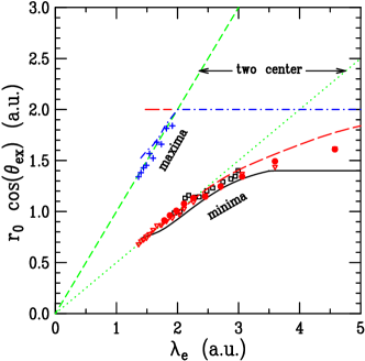
Figure 3: Recombination in geometry (I) for H₂. For the extrema in the photon-intensity orientation dependence, the projection of the bond length on the electron momentum direction, $r_{0}\cos(\theta_{ex})$, is plotted against the electron wavelength $\lambda_{e}$. The dotted (dashed) curve marks minima (maxima) due to two-centre emittance (see text). The solid curve represents minima for $r_{0}=1.4\,\,{\rm a.u.}$, whereas the long-dashed (dashed-dotted) curves represent minima (maxima) for $r_{0}=2\,\,{\rm a.u.}$. For comparison the extrema in the orientation dependence in HHG for time-dependent strong field calculations for model molecules lein02 are plotted as well: interference minima for ($\triangledown$) H${}^{+}_{2}$ at $r_{0}=2\,\,{\rm a.u.}$, laser intensity $I=10^{15}\,{\rm W}/{\rm cm}^{2}$; ($\bullet$) H${}^{+}_{2}$ at $r_{0}=2\,\,{\rm a.u.}$, $I=5\times 10^{14}\,{\rm W}/{\rm cm}^{2}$; ($\square$) H₂ at $r_{0}=1.4\,\,{\rm a.u.}$, $I=5\times 10^{14}\,{\rm W}/{\rm cm}^{2}$; ($+$) interference maxima for H${}^{+}_{2}$ at $r_{0}=2\,\,{\rm a.u.}$, $I=10^{15}\,{\rm W}/{\rm cm}^{2}$. Note that the present definition of $\lambda_{e}$ differs from lein02 .

A convenient way of analyzing the extrema is presented in Fig. 3 where the projection $r_{0}\cos(\theta_{ex})$ is plotted as a function of $\lambda_{e}$. Our results bear a strong resemblance to those of time-dependent strong field calculations of HHG in H₂ and H${}^{+}_{2}$ model molecules lein02 . This supports our prior assumption on that one can treat the recombination in HHG approximately as a weak-field process. Also, one finds the predictions made about the increase of $\delta_{\theta}$ towards parallel molecular orientation confirmed. Not surprisingly, the signature of two-center interference fades with increasing electron wavelength. However, at the electron wavelengths considered, this effect can be attributed mainly to the decreasing ratio of kinetic energy of the electron to the ionization threshold. In general, the orientation dependence of the recombination photon intensity for H₂ can be well described within the two-center interference model.

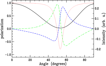
Figure 4: The H₂ molecule lies in the plane perpendicular to the photon propagation direction which is parallel to the z-axis in the Stokes parameters frame [geometry (II)]. The electron is here chosen to move along the x-axis. Shown is as solid curve the recombination photon intensity for $\lambda_{e}=1.6\,\,{\rm a.u.}$, $r_{0}=1.4\,\,{\rm a.u.}$ against the angle between the molecular axis and the propagation direction of the electron. Dotted, dashed-dotted and dashed curves are the Stokes parameters $p_{1}$, $p_{2}$ and $p_{3}$, respectively. These show strong variations in the vicinity of the minima.

As indicated, we can calculate all the Stokes parameters. In geometry (I), only linear photon polarization is possible. In geometry (II), however, where the molecular axis lies in the plane perpendicular to the photon propagation direction, the photon can have different polarizations and even circular polarization can be obtained (see Fig. 4). All polarizations show strong variations in the vicinity of the interference minimum. Otherwise only small polarization variations have been found. Thus, although the polarization depends on the geometry, the difference is small for H₂ because the signal is dominated by the polarization parallel to the electron momentum except in the small range around the interference minimum. This can be understood within the two-center model since the H₂ molecular orbital is approximately the sum of two atomic 1s-orbitals. These are spherically symmetric and therefore do not produce a signal polarized perpendicular to the electron momentum.

IV Results for N₂

Given the excellent agreement of our H₂ results with time-dependent strong field calculations lein02 we can move to a prediction for the orientation dependence of HHG from the N₂ $3\sigma_{g}$ valence orbital. The time-dependent HHG calculation for this system is quite complicated and has not been carried out.

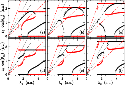
Figure 5: Projection $r_{0}\cos(\theta_{ex})$ versus electron wavelength $\lambda_{e}$ for molecular orientations $\theta_{ex}$ under which minima (x) and maxima (+) occur in the N₂ $3\sigma_{g}$ recombination photon intensity. The bond length $r_{0}$ is $1.768\,\,{\rm a.u.}$ in (a) and (d), $2.068\,\,{\rm a.u.}$ in (b) and (e) (ground-state bond length), and $2.368\,\,{\rm a.u.}$ in (c) and (f), respectively. The upper plots [(a), (b), (c)] show the positions of extrema when the molecule lies in the plane spanned by the electron and photon direction [geometry (I)], whereas the molecule rotates in the plane perpendicular to the photon direction in the lower plots (d), (e), (f) [geometry (II)]. The dotted (dashed) curve is the one for minima (maxima) according to the two-center interference model for p-orbital contributions. Note that minima and maxima are interchanged as compared to the s-orbital contributions. The dashed-dotted line marks minima according to $r_{0}\cos(\theta_{ex})=0.75\,\lambda_{e}$.

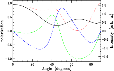
Figure 6: The N₂ molecule lies in the plane perpendicular to the photon propagation direction which is parallel to the z-axis in the Stokes parameters frame [geometry (II)]. The electron is here chosen to move along the x-axis. Shown is as solid curve the recombination photon intensity for $\lambda_{e}=1.6\,\,{\rm a.u.}$, $r_{0}=2.068\,\,{\rm a.u.}$ against the angle between the molecular axis and the propagation direction of the electron. Dotted, dashed-dotted and dashed curves are the Stokes parameters $p_{1}$, $p_{2}$ and $p_{3}$, respectively.

While both, H₂ $1\sigma_{g}$ and N₂ $3\sigma_{g}$, have the same symmetry, they are rather different otherwise. While $1\sigma_{g}$ is mainly built up from atomic s-orbitals and does not possess nodes, $3\sigma_{g}$ is dominated by atomic p-orbitals and has a more complex structure wahl66 . As a consequence the orientation dependence for N₂ $3\sigma_{g}$ is more complex than for H₂ $1\sigma_{g}$. As in the previous section, we have investigated geometries (I) and (II). In Fig. 5 the extrema for the equilibrium bond length $2.068\,{\rm a.u.}$ as well as for $1.768\,{\rm a.u.}$ and $2.368\,{\rm a.u.}$ are plotted. Contrary to H₂, there are big differences between the two geometries. Figure 6 shows the orientation dependence of the Stokes parameters for geometry (II). Large variations are found over a broader range of angles than in H₂, i.e., the component perpendicular to the electron momentum cannot be disregarded. At small angles, the signal is still dominated by the polarization parallel to the electron, but not so for larger angles.

Since N₂ is a homonuclear diatomic molecule we might expect to find two-center interference in the region where the wavelength of the electron equals approximately the internuclear distance. However, Fig. 5 shows that it is not straightforward to identify such signatures.

To understand the observed behavior, we first note that the two atomic p-orbitals “inside” the N₂ valence orbital are of course not spherically symmetric. Therefore, unlike s-orbitals, each of them can produce a substantial component polarized perpendicular to the electron momentum with a pronounced dependence on the molecular orientation. However, this component does not show up in geometry (I). This explains the difference between the two geometries. Furthermore, the molecular orbital is not constructed of atomic p-orbitals only, but we have an s-orbital admixture of about 30%. This makes the two-center interference picture problematic because different interference patterns are expected for the two orbital types: to ensure $\sigma_{g}$ symmetry, the two s-orbitals $\phi_{\rm s}(\mathbf{r}-\mathbf{r}_{0}/2)$ and $\phi_{\rm s}(\mathbf{r}+\mathbf{r}_{0}/2)$ are added with the same sign, so that interference conditions are obtained as described for H₂; the p-orbitals $\phi_{\rm p}(\mathbf{r}-\mathbf{r}_{0}/2)$ and $\phi_{\rm p}(\mathbf{r}+\mathbf{r}_{0}/2)$, on the other hand, are added with opposite signs, leading to an interchange of maxima and minima lein02 .

Clearly, the simultaneous presence of both types of interference will lead to a complicated orientation dependence. However, we can look for situations where either s- or p-orbitals dominate the signal. One such case is geometry (I) near an orientation of 90^o. Here, the individual p-orbitals generate a negligible signal due to their mirror antisymmetry, as is obvious when one considers a matrix element of the form $\langle\phi_{\rm p_{x}}(\mathbf{r})|z|\exp(ikz)\rangle$ where the incoming electron is approximated by a plane wave. Consequently, s-orbital contributions should dominate. In fact, Figs. 5(a)-(c) show that in the small-wavelength regime, geometry (I) yields local maxima at $\theta=90^{\rm o}$ as a consequence of constructive interference (similar to H₂). Another example is geometry (II), when only the component perpendicular to the electron momentum is measured. In this case, the s-orbital contributions are small as explained above in the context of H₂. Consequently, we should observe the p-type interference pattern, i.e., zero signal at 90^o and a series of minima and maxima when the angle is decreased. This is indeed the case for small electron wavelengths as is shown in Fig. 7 where the extrema for the perpendicular component are plotted. In this plot, the extrema are systematically slightly below the “perfect” two-center interference lines $r_{0}\cos(\theta_{ex})=n\,\lambda_{e}/2$. The total photon intensity in geometry (II) exhibits a similar behavior, see the lower panels of Fig. 5. This demonstrates the predominance of the p-orbital part even in the total signal.

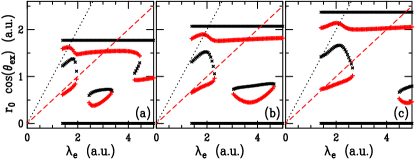
Figure 7: Same as Fig. 5 when only the component polarized perpendicular to the electron momentum is measured in geometry (II). (The molecular axis lies in a plane perpendicular to the the photon propagation direction.) The dotted (dashed) curve is the one for minima (maxima) according to the two-center interference model for p-orbital contributions.

In geometry (I) we have both s- and p-orbital contributions for the small and intermediate angles. Although in this regime the results cannot be explained in a simplified picture, we find a set of minima (see Fig. 5) following a straight line $r_{0}\cos(\theta_{ex})=0.75\,\lambda_{e}$ that lies just in the middle between the two-center interference lines.

V Conclusions

In conclusion, we have shown that the orientation dependence of the recombination photon intensity in H₂ can be described very well in a two-center interference model. Our results on the orientation dependence bear a remarkable resemblance with those obtained from the time-dependent Schrödinger equation for HHG lein02 . This shows that our method can be used alongside those others to obtain estimates about the effects of molecular geometry and orientation on the photon intensity in HHG. We have made such a prediction for the case of N₂. Furthermore, we have demonstrated, that the photons from HHG in oriented molecules do not exhibit only linear polarization. Rather, the polarization of those photons show strong variations and can even be circular, depending on the molecular orientation. For N₂, the interpretation of the results within a two-center interference picture is hampered by the fact that the valence orbital has admixtures of both atomic s- and p-orbitals, which produce different interference patterns. However, we have pointed out situations where one of the two orbital types dominates the signal so that interference can be observed.

References

- (1) F. Krausz, Phys. World 14, 41 (2001).
- (2) M. Hentschel, R. Kienberger, Ch. Spielmann, G. A. Reider, N. Milosevic, T. Brabec, U. Heinzmann, M. Drescher, and F. Krausz, Nature 414, 509 (2001).
- (3) P. B. Corkum, Phys. Rev. Lett. 71, 1994 (1993).
- (4) H. Niikura, F. Légaré, R. Hasbani, M. Yu Ivanov, D. M. Villeneuve, and P. B. Corkum, Nature 421 (2003).
- (5) R. Velotta, N. Hay, M. B. Mason, M. Castillejo, and J. P. Marangos, Phys. Rev. Lett. 87, 183901 (2001).
- (6) H. Yu and A. D. Bandrauk, Chem. Phys. 102, 1257 (1995); R. Kopold, W. Becker, and M. Kleber, Phys. Rev. A 58, 4022 (1998); D. G. Lappas and J. P. Marangos, J. Phys. B : At. Mol. Opt. Phys. 33, 4679 (2000).
- (7) R. R. Lucchese, G. Raseev, and V. McKoy, Phys. Rev. A 25, 2572 (1982).
- (8) K. Blum, Density Matrix and Its Application (Plenum Press, New York, 1981).
- (9) B. Zimmermann, Vollständige Experimente in der atomaren und molekularen Photoionisation, vol 13 in Studies of Vacuum and X-ray Processes edited by U. Becker (Wissenschaft und Technik Verlag, Berlin, 2000).
- (10) B. Lohmann, B. Zimmermann, H. Kleinpoppen, and U. Becker, Adv. At. Mol. Opt. Phys. 49, 218 (2003).
- (11) D. Dill, J. Chem. Phys. 65, 1130 (1976).
- (12) M. Lein, N. Hay, R. Velotta, J. P. Marangos, and P. L. Knight, Phys. Rev. A 66, 023805 (2002).
- (13) A. C. Wahl, Science 151, 961 (1966).