Integral analysis of laminar indirect free convection boundary layers with weak blowing for Schmidt no. $\sim$ 1

ABSTRACT

Laminar natural convection at unity Schmidt number over a horizontal surface with a weak normal velocity at the wall is studied using an integral analysis. To characterise the strength of the blowing, we define a non-dimensional parameter called the blowing parameter. After benchmarking with the no blowing case, the effect of the blowing parameter on boundary layer thickness, velocity and concentration profiles is obtained. Weak blowing is seen to increase the wall shear stress. For blowing parameters greater than unity, the diffusional flux at the wall becomes negligible and the flux is almost entirely due to the blowing.

Introduction

Fluid motion driven by an indirectly induced pressure gradient normal to the direction of the density potential difference is termed as indirect natural convection  [geb, ; blt, ]. An example is natural convection occurring over a horizontal heated surface. At large Grashoff numbers, the flow is of boundary layer type , and can be described by similarity solutions [gzc, ; rc, ]. Such boundary layers could form over a porous surface with blowing at the surface, the effect of which on the behavior of the boundary layer is not obvious. Previous investigations on the effect of blowing on indirect free convection boundary layers were conducted by Clarke & Riley  [cr, ] and Gill et.al. [gzc, ] using similarity analysis of the boundary layer equations. The boundary layer equations admit similarity solutions only for a restrictive and interdependent spatial distribution of wall velocity and density potential. Hence, the scope of these solutions is limited. We study indirect natural convection boundary layers for unity Schmidt(or Prandtl) number fluids, when a weak normal velocity is imposed at the wall. The wall velocity and density potential are not functions of horizontal distance. The imposed velocities are considered to be weak in the sense that they are of the order of vertical characteristic velocity in the boundary layer when no blowing is present. An integral method is used to obtain approximate solutions to the boundary layer equations for blowing velocities and wall concentrations that are constant in the horizontal direction.

The notation used is plain symbols for nondimensional variables, superscript $\,\tilde{}\,$ for dimensional variables and subscript c for characteristic scales. The paper is organised in the following manner. Using the characteristic scales in the problem,the boundary layer equations are derived. Integral equations are formulated by integrating the boundary layer equations across the boundary layer thickness, using profiles that satisfy the boundary conditions. The solution procedure of the resulting initial value problem is explained and the results are initially compared with the similarity solutions of Rotem and Classen [rc, ] for no blowing case. The effect of blowing on the boundary layer thickness, concentration and velocity profiles, and mass flux are studied.

Boundary layer approximation

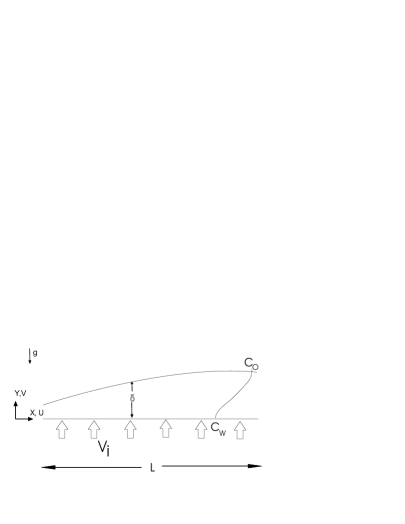
FIG. 1: Schematic of the problem studied

Consider a fluid having a concentration $\tilde{C}_{o}$ of some species above a horizontal porous surface maintained at $\tilde{C}_{w}$, with $\tilde{C}_{w}\,<\,\tilde{C}_{o}$. Also, a fluid with concentration $\tilde{C}_{w}$ flows through the surface with a normal velocity $\tilde{v}_{w}$. (The problem is equivalent to natural convection over a heated plate with blowing, with $\tilde{C}_{w}$ representing the wall temperature and $\tilde{C}_{o}$ the temperature of the ambient.) The geometry of the problem studied along with the variables used are shown in Figure (1). $\tilde{u},\,\tilde{v}$ are the velocity components in the $\tilde{x},\tilde{y}$ directions, and the boundary layer thickness is $\tilde{\delta}(\tilde{x})$.The wall velocity is considered to be independent of the density potential.

Let the characteristic length scales in the horizontal and vertical directions be $x_{c}=L,$ and $y_{c}=\delta_{c},$ a characteristic boundary layer thickness. L is taken as the horizontal dimension of the surface. Let $\,u_{c}\,\mathrm{and}\,v_{c}$ denote the characteristic horizontal and vertical velocities, $p_{c}$ the characteristic pressure and $c_{c}=\tilde{C}_{o}-\tilde{C}_{w}=\Delta\tilde{C}$ the characteristic concentration difference.

Following Rotem and Classen [rc, ], for $Sc\sim 1$

$$\delta_{c}\sim\frac{L}{Gr_{L}^{1/5}}\,,\;\;u_{c}\sim\frac{\nu}{L}Gr_{L}^{2/5}\,,\;\;v_{c}\sim\frac{\nu}{L}Gr_{L}^{1/5},\;\;p_{c}\sim\rho(\nu/L)^{2}Gr_{L}^{4/5}$$ (1)

where, $Gr_{L}\,=\frac{g\beta\Delta\tilde{C}L^{3}}{\nu^{2}}$, the Grashoff number. Here $g\,,\beta\,,\nu\,$ denote acceleration due to gravity, salinity volumetric expansion coefficient and kinematic viscosity respectively. The horizontal characteristic velocity scale can be rewritten as,

$$u_{c}\sim\sqrt{g\beta\Delta C\delta_{c}}\,,\;v_{c}\sim u_{c}\left(\delta_{c}/L\right),\;p_{c}\sim\rho u_{c}^{2}$$ (2)

$u_{c}$ can hence be viewed as a free fall velocity over the characteristic boundary layer thickness. The vertical characteristic velocity is $\delta_{c}/L$ times smaller than $u_{c}$ and the predominant balance is between motion pressure and the horizontal velocities. The motion pressure, $\tilde{p}\,=\,\tilde{p}_{s}-\tilde{p}_{h}$, where $\tilde{p}_{s}$ is the local static pressure in the presence of density variations, and $\tilde{p}_{h}$ is the local hydrostatic pressure when the fluid through out is at the reference density $\tilde{\rho}_{r}$.

Normalising the governing equations of two dimensional continuity, Navier-Stokes and species equation with these characteristic scales, dropping terms of order $\leq 1/Gr_{L}^{2/5}$ when $Gr_{L}\rightarrow\infty$, and assuming Schmidt number, $Sc\sim 1$ we obtain the non-dimensional boundary layer equations as,

$$\frac{\partial u}{\partial x}+\frac{\partial v}{\partial y}=0$$ (3)

$$u\frac{\partial u}{\partial x}+v\frac{\partial u}{\partial y}=-\frac{\partial p}{\partial x}+\frac{\partial^{2}u}{\partial y^{2}}$$ (4)

$$\frac{\partial p}{\partial y}=\,c$$ (5)

$$u\frac{\partial c}{\partial x}+v\frac{\partial c}{\partial y}=\frac{\partial^{2}c}{\partial y^{2}}$$ (6)

with the boundary conditions,

$$\textrm{at y =}\delta(x):\;\;\;u=0,\quad\frac{\partial u}{\partial y}=0,\qquad c=\,0,\qquad\frac{\partial c}{\partial y}=0$$ (7)

$$\textrm{at y = 0}:\quad u=0,\quad c=1\quad v=\frac{\tilde{v}_{w}}{v_{c}}\,=\,\frac{Re_{w}}{Gr_{L}^{1/5}}\,=V_{w},$$ (8)

where $x=\tilde{x}/L,\,y=\tilde{y}/\delta_{c},\,u=\tilde{u}/u_{c},\,v=\tilde{v}/v_{c},\,p=\tilde{p}/p_{c},\,c\,=\,\frac{\tilde{C_{o}}-\tilde{c}}{\Delta\tilde{C}},\,\delta(x)\,=\,\tilde{\delta}(\tilde{x})/\delta_{c},\;Re_{w}=\tilde{v}_{w}L/\nu$. Equation (5) shows that the vertical concentration distribution creates a vertical pressure distribution, the horizontal gradient of which in (4) drives the flow. The concentration distribution is, in turn, a result of this motion as well as diffusion.

The Blowing parameter $V_{w}$ is the non-dimensional normal velocity at the wall. The blowing parameter also shows the condition for similarity of the boundary layers in the presence of a weak blowing. When the normal velocity at the wall has a dependence of $\tilde{v}_{w}\,\sim\,\tilde{x}^{-2/5}$ the boundary condition become independent of $\tilde{x}$ and a similarity solution can be obtained. The normalised terms in the boundary layer equations are of order one. Hence these approximate equations can be expected to hold till the blowing parameter $\frac{Re_{w}}{Gr_{L}^{1/5}}\,\sim$ O(1). We restrict our calculations up to $V_{w}\,=\,3$.

Integral Formulation

Consider a steady laminar indirect natural convection boundary layer with a weak blowing that could be described by the boundary layer equations (3) - (8). Integrating  (3) from the surface to $\delta(x)$ and applying the boundary conditions, we get the non dimensional integral mass conservation equation as

$$\frac{d}{dx}\int_{0}^{\delta(x)}u\;dy+v_{\delta}-V_{w}=0$$ (9)

where, $v_{\delta}=\tilde{v}_{\delta}/v_{c}$ is the non-dimensional entrainment velocity at the edge of the boundary layer. The non-dimensional integral x momentum equation is obtained by integrating the equation obtained after multiplying  (3) by u and subtracting  (4).

$$\frac{d}{dx}\int_{0}^{\delta(x)}u^{2}\;dy+\int_{0}^{\delta(x)}\frac{\partial p}{\partial x}\;dy+\frac{\partial u}{\partial y}_{|_{y=0}}=0$$ (10)

This equation expresses a balance of horizontal momentum flux with horizontal pressure gradient and wall shear stress. Integrating  (6) from 0 to $\delta(x)$ and substituting for $v_{\delta}$ from  (9), the non-dimensional integral species equation is obtained as

$$-\frac{d}{dx}\int_{0}^{\delta(x)}uc\;dy+\frac{\partial c}{\partial y}_{|_{y=0}}\,+V_{w}\,=\,0$$ (11)

The terms in the above equation represent convection by the horizontal velocity and entrainment from ambient, the diffusive flux at the wall and the blowing flux at the wall respectively. The concentration profile is approximated by the function,

$$f(\eta,a)\,=\,c\,={\left(1-\eta\right)}^{2}\,\left(1+a\,\eta\right)$$ (12)

where, $\eta\,=\,\tilde{y}/\tilde{\delta}(\tilde{x})$ and the coefficient a captures the non similar nature of the profile in the presence of blowing. The profile  (12) satisfies the boundary conditions  (7) and  (8) ie., $f(0,a)=1,\>f(1,a)=0,\;\dot{f}(1,a)=0$, where, superscript . denote differentiation with respect to $\eta$.

The coefficient $a$ in (12) is found from the condition that the profile satisfies the species equation  (6) at the wall ie,

$$\ddot{f}(0,a)=V_{w}\,\delta\dot{f}(0,a)$$ (13)

Substituting the values of $\dot{f}(0,a)\,=\,a-2\,\mathrm{and}\,\ddot{f}(0,a)\,=\,2-4a$ in  (13) and solving for $a$,we get

$$a(V_{w},x)=2-\frac{6}{4+V_{w}\,\delta}$$ (14)

The velocity profile is approximated by the polynomial

$$u(\eta,{b})\,=\,c_{1}\,+{b}(x)\,\eta\,+\,c_{2}\,\eta^{2}\,+\,c_{3}\,\eta^{3}\,+\,c_{4}\,\eta^{5}$$ (15)

where the dimensionless coefficient b captures the non similar nature of the profile in the presence of blowing. We need to satisfy the boundary conditions  (7) and  (8), ie. $u(0,{b})\,=0,\>u(1,{b})\,=0,\>\textrm{and}\>\dot{u}(1,{b})\,=0,$ and the condition obtained from the x-momentum equation at the wall,

$$\frac{V_{w}}{\delta}\dot{u}(0)-\left(\delta\,I_{1}\right)^{\prime}\,-\frac{\ddot{u}(0)}{\delta^{2}}=0$$ (16)

where ^′ denotes differentiation with respect to x. In the above equation, the horizontal pressure gradient in  (4) is expressed in terms of the concentration profile using  (5) as

$$\left.\frac{dp}{dx}\right|_{\eta=0}\,=\,-(\delta I_{1})^{\prime}\,\;\textrm{ where,}\,I_{1}\,=\,\int_{0}^{1}\,f(\eta)d\eta$$ (17)

Using the above conditions, $c_{1}\,=\,0$, and $\,c_{2},\,c_{3},\,c_{4}\,$ can be expressed as functions of $b,\,V_{w},\,\textrm{and}\,\delta$. The final expressions of the coefficients are given in the Appendix. The velocity profile is obtained as

$$\raggedleft u(\eta,b)\,=\,\eta\,(\eta-1)^{2}\left[\frac{b(x)}{2}\,\left(2+\eta(4+V_{w}\,\delta)\right)-\frac{\eta(2+V_{w}\,{\delta})(6+V_{w}\,\delta)}{4(4+V_{w}\,\delta)^{2}}\,\delta^{2}\delta^{\prime}\right]\@add@raggedleft$$ (18)

Rewriting  (11) and  (10) in terms of the profiles  (12) and  (15), we get the integral equations for species and momentum.

$$\left[\delta\,I_{uf}\right]^{\prime}-V_{w}+\frac{\dot{f}(0,a)}{\delta}=0$$ (19)

$$\left[\,\delta\,I_{u^{2}}\,-\delta^{2}\,I_{2}\right]^{\prime}+\frac{\dot{u}(0,b)}{\delta}\,=\,0$$ (20)

where,

$$I_{uf}=\int_{0}^{1}u(\eta,x)\,f(\eta,a)\,d\eta,\;I_{u^{2}}=\int_{0}^{1}u(\eta,b)^{2}\,d\eta;\>I_{2}\,=\,\int_{0}^{1}\,\int_{\eta}^{1}f(\eta,a)\,d\eta\>d\eta$$ (21)

In  (20) above, the horizontal pressure gradient in  (10) has been replaced in terms of the concentration profile by integrating the y momentum equation  (5) from $1\,\textrm{to}\,\eta$ as below

$$\int_{0}^{\delta(x)}\frac{\partial p}{\partial x}\;dy=\,-(\delta^{2}\,I_{2})^{\prime}$$ (22)

Substituting the values ${I}_{uf},\,{I}_{u^{2}},\,{I}_{2},\,\dot{u}(0),\,\dot{{f}}(0)$ and simplifying, we get two autonomous nonlinear second order ordinary differential equations for the unknowns $\delta(x)$ and $b(x)$ as follows.

$${\delta}^{\prime\prime}\,+\,{\delta}^{\prime}\left(A\,{\delta}^{\prime}+\,B\right)+\,C\,{b}^{\prime}\,+\,D\,=\,0$$ (23)

$${\delta}^{\prime\prime}\left(1+E{\delta}^{\prime}\right)\,+\,{\delta}^{\prime}\left(\,F\,{\delta}^{\prime^{2}}\,+\,G\,{\delta}^{\prime}\,+\,H\right)+\,{b}^{\prime}\left(I{\delta}^{\prime}\,+J\right)+\,K=0$$ (24)

where the coefficients, A to K are nonlinear functions of ${\delta}(x),\,V_{w}\,\textrm{and}\,{b}(x)$ The expressions for these coefficients are given in the Appendix.

Equations  (23) and  (24) needs three initial conditions ${\delta}(0),\,{\delta}^{\prime}(0),$ and ${b}(0)$ for solution as an initial value problem. We assume that as $x\rightarrow 0$ the boundary layer behaves similar to the case with no blowing. This is equivalent to assuming an infinitesimal distance where no blowing effects are present. Hence, we use the values of ${\delta}(\epsilon)\,=\,0.0179,\,{\delta}^{\prime}(\epsilon)\,=\,6369.7$ and ${b}(\epsilon)\,=\,0.2358$, where $\epsilon=10^{-6}$, as calculated from the similarity solutions of Rotem and Classen [rc, ]as the initial conditions. It was found that the solution was insensitive to changes in initial conditions up to an order magnitude from the above conditions. The NDSolve routine of MATHEMATICA was used to numerically solve  (23) and  (24) simultaneously.

Results and Discussion

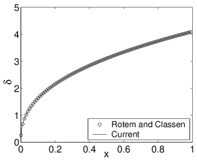
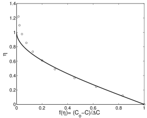
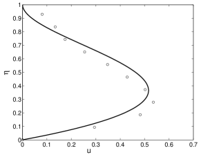
FIG. 2: Comparison with Rotem and Classen [rc, ] for no blowing case. (a) Non dimensional boundary layer thickness (b) Non-dimensional concentration profile (c) Non-dimensional Velocity profile

The results are initially compared with similarity solutions for the no blowing case by Rotem and Classen [rc, ]. The integral analysis gives ${\delta}(x)\,\sim\,x^{2/5}$, same as that obtained in the similarity solution. The boundary layer thickness $\delta$ in the integral analysis is equal to the thickness at which c = 0.05 in the solution of Rotem and Classen  [rc, ]. Figure (2) compares the $x$ dependence of the non dimensional boundary layer thickness $\delta$ with that of Rotem and Classen [rc, ].Figures (2) and  (2) compare the concentration and velocity profiles obtained from the integral analysis with those from the similarity solution. Considering the approximate nature of integral methods, the comparison is satisfactory.

Figure (3) shows the effect of blowing on the boundary layer thickness. As expected, higher blowing results in larger boundary layer thickness; the increase in total added fluid increases the boundary layer thickness.

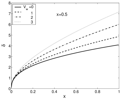
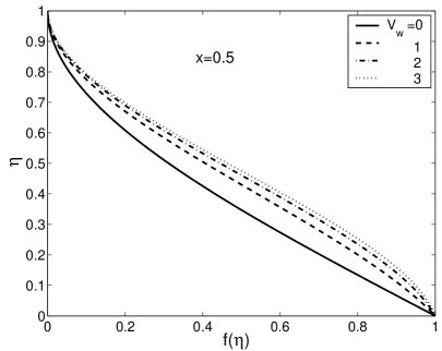
FIG. 3: Effect of blowing on (a) boundary layer thickness and (b) concentration profile

The concentration profiles at $x=0.5$ for different blowing parameters are shown in Figure (3). The reduction in the gradient of concentration at the wall shows that the diffusive flux decreases with increase in the blowing parameter.

The major effect of the change in concentration profile shape is on the pressure distribution. The motion pressure outside the boundary layer is zero. The motion pressure within the boundary layer is given by $\tilde{p}(\tilde{y},\tilde{x})=-\rho g\beta\int_{\tilde{y}}^{\tilde{y}=\tilde{\delta}}(\tilde{C}_{o}-\tilde{c})\,d\tilde{y}$. Presence of increased amounts lighter fluid in the boundary layer due to blowing results in larger value of $\tilde{C}_{o}-\tilde{c}$. This results in a larger favourable horizontal pressure difference with the outside motion pressure than in the case of without blowing, resulting in larger velocities. This could be observed in Figure (4) shows the non dimensional horizontal velocity distribution for different blowing parameters at x=0.5. Figure 4 shows the variation of horizontal pressure gradient at the wall as a function of horizontal distance for increasing value of the blowing parameter. The pressure gradient was calculated using the relation $\frac{d\tilde{p}}{d\tilde{x}}=-\rho g\beta\frac{d}{d\tilde{x}}\int_{\tilde{y}=0}^{\tilde{y}~{}=~{}\tilde{\delta}}(\tilde{C}_{o}-\tilde{c})d\tilde{y}$. The increased amounts of lighter fluid in the boundary layer has the effect of making the horizontal pressure gradient at the wall more favourable. This increases $\frac{d\tilde{u}}{d\tilde{y}}$ at the wall and results in increased wall shear stresses with blowing. This behaviour is in contrast to what is observed in a shear boundary layer with blowing. For example, in the case of the Blasius boundary layer, blowing reduces the wall shear stress.

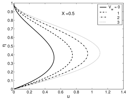
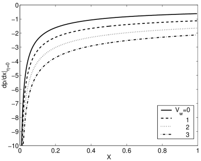
FIG. 4: Effect of blowing on (a)horizontal velocity profile and (b)horizontal pressure gradient at the wall

The vertical characteristic velocity in the boundary layer is $\frac{\delta_{c}}{L}$ times the horizontal characteristic velocity, as can be seen from Equation (2). Therefore, the vertical momentum from blowing velocities of the order of $v_{c}\>ie,\>V_{w}\,\sim\,O(1)$, doesn’t seem to be sufficient to cause a change in the near wall linearity of the horizontal velocity profile. For the current range of blowing parameters investigated, the major effect seems to be due to increase in motion pressure, which increases the horizontal velocities, and the wall shear stress.

The total mass flux of the species into the boundary layer is

$$\tilde{q}\,=\,\tilde{v}_{w}\,\Delta\tilde{C}\,+\,D\frac{\partial\tilde{c}}{\partial\tilde{y}}|_{\tilde{y}=0}$$ (25)

The first term on the right hand side of  (25) is due to blowing(advection) and the second term represents diffusion. The non-dimensional flux is,

$$q\,=\,\frac{\tilde{q}}{D\frac{\Delta C}{\delta_{c}}}\,=\,V_{w}\,-\,\frac{f^{\prime}(0)}{{\delta}}$$ (26)

The variation of non-dimensional diffusive flux over the length of the boundary layer is shown in Figure(5) 6. Blowing reduces the diffusive flux. Note that when $V_{w}\,>\,1$, except very near the leading edge, the diffusive flux is an order lower than the blowing flux, which is equal to $V_{w}$.

Figure (6) shows the longitudinally averaged blowing and diffusive fluxes as a function of $V_{w}$. The total flux is also shown in the figure. As pointed above, the mean diffusive flux drops with $V_{w}$. At $V_{w}\,=\,3,$ the diffusive flux is about $\frac{1}{3}$rd the diffusive flux at no blowing. The blowing flux increases linearly with the blowing parameter, and at $V_{w}\,=\,3,$ the blowing flux is about fifteen times the diffusive flux, and about 5 times the no blowing flux. The variation of the ratio of the total flux with blowing to the flux without blowing ($\frac{q}{\frac{f^{\prime}(0)}{\delta}}$) could also be noticed from Figure (6). For example, the flux with $V_{w}$=1 is double the flux with no blowing. To take a specific example, this means that at a commonly encountered $Gr_{L}=10^{6}$ in water, blowing velocities of the order of 1 mm/s doubles the flux from the no blowing case. Hence, weak blowing increases the flux appreciably over the corresponding no blowing flux.

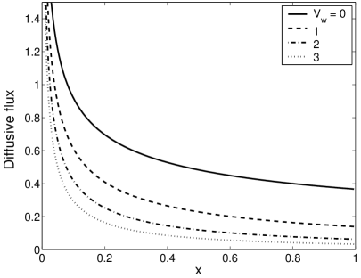
FIG. 5: Variation of the longitudinal distribution of diffusive flux with blowing parameter

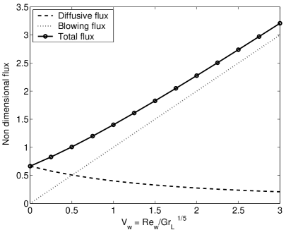
FIG. 6: Variation of non-dimensional fluxes with blowing parameter

Conclusions

The integral analysis developed in this paper is used to study the effects of weak blowing on indirect laminar natural convection boundary layers. The blowing velocity and wall concentration are constant along the wall. The analysis is subject to the assumptions of small $\delta/L$(large Grashoff numbers), unity Schmidt(or Prandtl) numbers and blowing velocities of the same order as the vertical characteristic velocities due to free convection in the boundary layer. Approximate solutions were obtained by numerically solving the integrated boundary layer equations. Following are the major conclusions from the study: (a) As expected, the boundary layer thickness increases with blowing (Figure 3). (b) Weak blowing increases the horizontal velocities in the boundary layer, resulting in the wall shear stress also increasing with blowing (Figure 4). (c) The concentration gradient at the wall and thus the diffusive flux reduces with increase in the blowing parameter (Figure 3). (d) For $V_{w}>1$, the flux due to advection caused by blowing becomes the predominant contribution to the total flux and hence the total flux shows a linear dependence on $V_{w}$. (e) Comparison of total flux with that in the case of no blowing show that a weak blowing results in considerable increase in flux (Figure 6).

Appendix

The coefficients in the velocity profile  (15) are,

$$c2=5\,{\delta}\,\,{b}-\,Q\,{\delta}^{2}\,{\delta}^{\prime},\quad c3=-{b}\,\left(3+10\,{\delta}\right)+2\,Q\,{\delta}^{2}\,{\delta}^{\prime},\quad c4=\frac{{b}\,\left(4+10\,{\delta}\right)}{2}-\,Q\,{\delta}^{2}\,{\delta}^{\prime}$$ (27)

$$\textrm{where},\>Q\,=\,\frac{\left(2+10\,{\delta}\right)\,\left(6+10\,{\delta}\right)\,}{4\,{\left(4+10\,{\delta}\right)}^{2}}$$ (28)

The coefficients in the differential equations  (23) and  (24) are obtained as

$$A=\frac{3}{\delta}+V_{w}\,\left(\frac{1}{2+V_{w}\,{\delta}}-\frac{3}{4+V_{w}\,{\delta}}+\frac{1}{6+V_{w}\,{\delta}}+\frac{7}{19+7\,V_{w}\,{\delta}}\right)$$ (29)

$$B=\frac{-2\,{b}\,\left(4+V_{w}\,{\delta}\right)\,\left(816+7\,V_{w}\,{\delta}\,\left(104+V_{w}\,{\delta}\,\left(25+2\,V_{w}\,{\delta}\right)\right)\right)}{{{\delta}}^{3}\,\left(2+V_{w}\,{\delta}\right)\,\left(6+V_{w}\,{\delta}\right)\,\left(19+7\,V_{w}\,{\delta}\right)}$$ (30)

$$C=\frac{-2\,{\left(4+V_{w}\,{\delta}\right)}^{2}\,\left(204+7\,V_{w}\,{\delta}\,\left(13+V_{w}\,{\delta}\right)\right)}{{{\delta}}^{2}\,\left(2+V_{w}\,{\delta}\right)\,\left(6+V_{w}\,{\delta}\right)\,\left(19+7\,V_{w}\,{\delta}\right)},\quad D=\frac{1680\,{\left(4+V_{w}\,{\delta}\right)}^{2}\,\left(6+V_{w}\,{\delta}\,\left(4+V_{w}\,{\delta}\right)\right)}{{{\delta}}^{4}\,\left(2+V_{w}\,{\delta}\right)\,\left(6+V_{w}\,{\delta}\right)\,\left(19+7\,V_{w}\,{\delta}\right)}$$ (31)

$$E=-\frac{{{\delta}}^{2}\,\left(2+V_{w}\,{\delta}\right)\,\left(6+V_{w}\,{\delta}\right)}{{b}\,{\left(4+V_{w}\,{\delta}\right)}^{2}\,\left(17+2\,V_{w}\,{\delta}\right)},\quad F=-\frac{-\delta\,\left(240+V_{w}\,{\delta}\,\left(236+5\,V_{w}\,{\delta}\,\left(12+V_{w}\,{\delta}\right)\right)\right)}{2\,{b}\,{\left(4+V_{w}\,{\delta}\right)}^{3}\,\left(17+2\,V_{w}\,{\delta}\right)}$$ (32)

$$G=\frac{3}{{\delta}}+V_{w}\,\left(\frac{1}{2+V_{w}\,{\delta}}-\frac{2}{4+V_{w}\,{\delta}}+\frac{1}{6+V_{w}\,{\delta}}+\frac{2}{17+2\,V_{w}\,{\delta}}\right)$$ (33)

$$H=\frac{504\,{\delta}\,\left(2+V_{w}\,{\delta}\right)\,\left(16+3\,V_{w}\,{\delta}\right)}{{b\,{\delta}^{3}\,\left(2+V_{w}\,{\delta}\right)\,\left(6+V_{w}\,{\delta}\right)\,\left(17+2\,V_{w}\,{\delta}\right)}}$$

$$-\frac{2\,{b}^{2}\,\left(4+V_{w}\,{\delta}\right)^{2}\,\left(76+V_{w}\,{\delta}\,\left(34+3\,V_{w}\,{\delta}\right)\right)}{{b\,{\delta}^{3}\,\left(2+V_{w}\,{\delta}\right)\,\left(6+V_{w}\,{\delta}\right)\,\left(17+2\,V_{w}\,{\delta}\right)}}$$ (34)

$$I=\frac{1}{{b}},\quad J=\frac{-4\,{\left(4+V_{w}\,{\delta}\right)}^{2}\,\left(76+V_{w}\,{\delta}\,\left(17+V_{w}\,{\delta}\right)\right)}{{{\delta}}^{2}\,\left(2+V_{w}\,{\delta}\right)\,\left(6+V_{w}\,{\delta}\right)\,\left(17+2\,V_{w}\,{\delta}\right)}$$ (35)

$$K=\frac{-5040\,{\left(4+V_{w}\,{\delta}\right)}^{2}}{{{\delta}}^{4}\,\left(2+V_{w}\,{\delta}\right)\,\left(6+V_{w}\,{\delta}\right)\,\left(17+2\,V_{w}\,{\delta}\right)}$$ (36)

References

- [1] B.Gebhartet.al. Buoyancy induced flows and transport. Hemisphere Publishing (1988).
- [2] H. Schlichting and K. Gersten. Boundary layer theory. Springer-Verlag (2000).
- [3] D. Gill, W.N. Zeh and E. Casal. Free convection on a horizontal plate. Z. Angew. Math. Phys. Vol 16(1965), pp 539.
- [4] Z. Rotem and L. Claassen. Natural convection above unconfined horizontal surfaces. Jl. Fluid. Mech. 39, part1(1969), pp 173.
- [5] J. Clarke and N. Riley. Natural convection induced in a gas by the presence of a hot porous horizontal surface. Ql. Jl. Mech. appl. Math. XXVIII, Pt.4(1975), pp 375.