On-Shell Description of Stationary Flames

Abstract

The problem of non-perturbative description of stationary flames with arbitrary gas expansion is considered. On the basis of the Thomson circulation theorem an implicit integral of the flow equations is constructed. With the help of this integral, a simple explicit expression for the vortex mode of the burnt gas flow near the flame front is obtained. Furthermore, a dispersion relation for the potential mode at the flame front is written down, thus reducing the initial system of bulk equations and jump conditions for the flow variables to a set of integro-differential equations for the flame front position and the flow velocity at the front. The developed approach is applied to the case of thin flames. Finally, an asymptotic expansion of the derived equations is carried out in the case $\theta\to 1$ where $\theta$ is the gas expansion coefficient, and a single equation for the front position is obtained in the second post-Sivashinsky approximation. It is demonstrated, in particular, how the well-known problem of correct normalization of the front velocity is resolved in the new approach. It is verified also that in the first post-Sivashinsky approximation, the new equation reduces to the Sivashinsky-Clavin equation corrected according to Cambray and Joulin. Analytical solutions of the derived equations are found, and compared with the results of numerical simulations.

I Introduction

The process of flame propagation presents an extremely complicated mathematical problem. The governing equations include the nonlinear flow equations for the fuel and the products of combustion, as well as the transfer equations governing the heat conduction and species diffusion inside the flame front. Fortunately, in practice, an inner flame scale determined by the latter processes is large compared to the flame front thickness, implying that the flame can be considered as a gasdynamic discontinuity. The initial problem is reduced thereby to a purely hydrodynamic problem of determining the propagation of a surface of discontinuity in an incompressible fluid, the laws of this propagation given by the usual Navier-Stokes and continuity equations complemented by the jump conditions at the surface, expressing the mass and momentum conservation across the flame front. The asymptotic methods^1-3 allow one to express these conditions in the form of a power series with respect to the small flame front thickness.

Despite this considerable progress, however, a closed theoretical description of the flame propagation is still lacking. What is meant by the term “closed description” here is the description of flame dynamics as dynamics of the flow variables on the flame front surface. Reduction of the system of bulk equations and jump conditions, mentioned above, to this “surface dynamics” implies solving the flow equations for the fuel and the combustion products, satisfying given boundary conditions and the jump conditions at the flame front, and has only been carried out asymptotically for the case $\theta\to 1,$ where $\theta$ is the gas expansion coefficient defined as the ratio of the fuel density and the density of burnt matter$.^{1,4-6}$

Difficulties encountered in trying to obtain a closed description of flames are conditioned by the following two crucial aspects:

(1) Characterized by the flow velocities which are typically well below the speed of sound, deflagration represents an essentially nonlocal process, in the sense that the flame-induced gas flows, both up- and downstream, strongly affect the flame front structure itself. A seeding role in this reciprocal process is played by the Landau-Darrieus (LD) instability of zero thickness flames$.^{7,8}$ A very important factor of non-locality of the flame propagation is the vorticity production in the flame, which highly complicates the flow structure downstream. In particular, the local relation between pressure and velocity fields upstream, expressed by the Bernoulli equation, no longer holds for the flow variables downstream.

(2) Deflagration is a highly nonlinear process which requires an adequate non-perturba-
tive description of flames with arbitrary values of the flame front slope. As a result of development of the LD-instability, exponentially growing perturbations with arbitrary wavelengths make any initially smooth flame front configuration corrugated. Characteristic size of the resulting “cellular” structure is of the order of the cutoff wavelength $L_{c}\sim 20L_{\rm f}$ given by the linear theory of the LD-instability$;^{3}$ $L_{\rm f}$ is the flame front thickness. The exponential growth of unstable modes is ultimately suppressed by the nonlinear effects. Since for arbitrary $\theta$ the governing equations do not contain small parameters, it is clear that the LD-instability can only be suppressed by the nonlinear effects if the latter are not small, and therefore so is the flame front slope.

The stabilizing role of the nonlinear effects is best illustrated in the case of stationary flame propagation. Numerical experiments⁹ on 2D flames with $\theta=6-8$ show that even in very narrow tubes (tube width of the order $L_{c}$), typical values for the flame front slope are about $1.5-2.0.$ Nonlinearity can be considered small only in the case of small gas expansion, $\theta\to 1,$ where one has the $O(\theta-1)$ estimate for the slope, so that it is possible to derive an equation^4-6 for the flame front position in the framework of the perturbation expansion in powers of $(\theta-1).$

This perturbative method gives results in a reasonable agreement with the experiment only for flames with $\theta\leq 3,$ propagating in very narrow tubes (tube width of the order $L_{c}$), so that the front slope does not exceed unity. Flames of practical importance, however, have $\theta$ up to 10, and propagate in tubes much wider than $L_{c}.$ As a result of development of the LD-instability, such flames turn out to be highly curved, which leads to a noticeable increase of the flame velocity. In connection with this, a natural question arises whether it is possible to develop a non-perturbative approach to the flame dynamics, closed in the sense mentioned above, which would be applicable to flames with arbitrary gas expansion.

A deeper root of this problem is the following dilemma: As was mentioned above, the flame propagation is an essentially non-local process; on the other hand, this non-locality itself is determined by the flame front configuration and the structure of gas flows near the front, so the question is whether an explicit bulk structure of the flow downstream is necessary in deriving an equation for the flame front position. In other words, we look for an approach that would provide a closed description of flames more directly, without the need to solve the flow equations explicitly.

The purpose of this paper is to develop such approach in the stationary case.

The paper is organized as follows. The flow equations and related results needed in our investigation are displayed in Sec. II.1. A formal integral of the flow equations is derived in Sec. II.2 on the basis of the Thomson circulation theorem. With the help of this integral, an expression for the vortex mode of the burnt gas flow near the flame front is obtained in Sec. III. To close the system of equations relating the flow variables on the flame front, potentiality of the flow upstream, and of the burnt gas flow after extracting the vortex mode are to be expressed through the values of the fuel velocity at the front. This is done in Sec. IV.1.1 in the form of dispersion relations, using which we obtain an equation relating the fuel velocity at the front and the front configuration in Sec. IV.1.2. Complemented by the relation defining the local burning rate (the evolution equation), the found equation provides description of stationary flames, which is closed in the above-mentioned sense. The developed approach is applied to the particular case of zero-thickness flames in Sec. IV.2.1. Furthermore, it is shown in Sec. IV.2.2 how effects related to the finite flame front thickness can be taken into account in the obtained equation. Finally, the case of weak gas expansion is considered in Sec. V, where a single equation for the flame front position is obtained in the third and the fourth orders in $(\theta-1).$ Analytical solutions of the third- and fourth-order equations are found in Secs. V.1.2 and V.2.2. The results obtained are discussed in Sec. VI. Appendix A contains a consistency check for the expression of the vortex mode, derived in Sec. III. Some auxiliary mathematical results used in the text are summarized in Appendix B.

II Integral representation of flow dynamics

As was mentioned in the point (1) of Introduction, an important factor of the flow non-locality downstream is the vorticity production in curved flames, which highly complicates relations between the flow variables. In the presence of vorticity, pressure is expressed through the velocity field by an integral relation, its kernel being the Green function of the Laplace operator. It should be noted, however, that the jump condition for the pressure across the flame front only serves as the boundary condition for determining an appropriate Green function, being useless in other respects. Thus, it is convenient to exclude pressure from our consideration from the very beginning. The basis for this is provided by the well-known Thomson circulation theorem. Thus, we begin in Sec. II.1 with the standard formulation of the problem of flame propagation, and then construct a formal implicit solution of the flow equations with the help of this theorem in Sec. II.2.

II.1 Flow equations

Let us consider a 2D stationary flame propagating in an initially uniform premixed ideal fluid. Let the Cartesian coordinates $(x,y)$ be chosen so that the $y$-axis is in the direction of flame propagation, $y=-\infty$ being in the fresh fuel. It will be convenient to introduce the following dimensionless variables

$$(\eta,\xi)=(x/R,y/R)\,,\ (w,u)=({\rm v}_{x}/U_{\rm f}\,,{\rm v}_{y}/U_{\rm f})\,,$$

$$\Pi=(P-{P}_{\rm f})/{\rho}_{-}{U_{\rm f}}^{2},$$

where $U_{\rm f}$ is the velocity of a plane flame front, $P_{\rm f}$ is the initial pressure in the fuel far ahead of the flame front, and $R$ is some characteristic length of the problem (e.g., the tube width). The fluid density will be normalized on the fuel density $\rho_{-}.$

As numerical experiments show, stationary flames exist only in sufficiently narrow tubes. Hence, assuming the tube walls ideal, and denoting its width by $b,$ we will deal below with spatially $2b$-periodic flames. More precisely, given a flame configuration described by the functions $f(\eta),w(\eta,\xi),u(\eta,\xi),$ $\eta\in[0,+b],$ where $f(\eta)$ denotes the flame front position, using the boundary conditions $f^{\prime}=0,w=0$ for $\eta=0,b,$ we continue this solution to the domain $\eta\in[-b,0]$ according to

$$f(\eta)=f(-\eta)\,,\qquad w(\eta,\xi)=-w(-\eta,\xi)\,,\qquad u(\eta,\xi)=u(-\eta,\xi)\,,$$ (1)

and then periodically continue it to the whole $\eta$-axis.

In connection with this procedure the following circumstance should be emphasized. All subsequent analysis is carried out under assumption that there exists a short wavelength cut-off for the flame perturbations. In other words, we consider flames with small but non-zero front thickness$.^{10}$ Existence of such a cut-off ensures smoothness of the functions under consideration. In particular, it prevents development of singularities such as the edge points occurring at the front of a zero-thickness flame, which lead to discontinuities in the values of the flow variables or their derivatives. The end points of the flame front, however, still represent a potential source of such discontinuities even in the case of flames with non-zero thickness because of the possibility of stream line refraction at these points, resulting in a formation of stagnation zones in the flow of burnt matter (see Ref. 11 for more detail). Having imposed the boundary condition $f^{\prime}(0)=f^{\prime}(b)=0$ we thereby exclude this possibility. In view of what has just been said, it is natural to assume further that considered as functions of the complex argument, $f(\eta)$ together with the “on-shell” values of the flow velocity, $w(\eta,f(\eta)),$ $u(\eta,f(\eta)),$ are analytical functions of $\eta$ in a vicinity of the real axis. This assumption, simplifying subsequent analysis, is only technical, and can be weakened if necessary.

As always, we assume that the process of flame propagation is nearly isobaric. Then the velocity and pressure fields obey the following equations in the bulk

$$\frac{\partial v_{i}}{\partial\zeta_{i}} = 0\,,$$ (2)

$$v_{i}\frac{\partial v_{k}}{\partial\zeta_{i}} = -\frac{1}{\rho}\frac{\partial\Pi}{\partial\zeta_{k}}\,,\quad k=1,2,$$ (3)

where $(\zeta_{1},\zeta_{2})=(\eta,\xi),\,(v_{1},v_{2})=(w,u),$ and summation over repeated indices is implied.

Acting on Eq. (3) by the operator $\varepsilon_{kl}\partial/\partial\zeta_{l},$ where $\varepsilon_{ik}=-\varepsilon_{ki},\ \varepsilon_{12}=+1,$ and using Eq. (2), one obtains a 2D version of the Thomson circulation theorem

$$v_{i}\frac{\partial\sigma}{\partial\zeta_{i}}=0\,,$$ (4)

where

$$\sigma\equiv\frac{\partial u}{\partial\eta}-\frac{\partial w}{\partial\xi}\,.$$

According to Eq. (4), the vorticity $\sigma$ is conserved along the stream lines. As a simple consequence of this theorem, one can find the general solution of the flow equations upstream. Namely, since the flow is potential at $\xi=-\infty$ ($u=V={\rm const},$ $w=0,$ where $V$ is the velocity of the flame in the rest frame of reference of the fuel), it is potential for every $\xi<f(\eta).$ Therefore,

$$u = \sum\limits_{n=-\infty}^{+\infty}~{}u^{(n)}\exp\left\{\frac{\pi}{b}(|n|\xi+in\eta)\right\}\,,\quad u^{(0)}=V\,,$$ (5)

$$w = \hat{H}(u-u^{(0)})\,,$$ (6)

where the linear Hilbert operator $\hat{H}$ is defined by

$$\hat{H}\exp(ik\eta)=i\chi(k)\exp(ik\eta)\,,\quad k\neq 0\,,$$ (7)

and

$$\chi(x)=\left\{\begin{array}[]{cc}+1,&x>0\,,\\ -1,&x<0\,.\end{array}\right.$$

In the coordinate representation, $\hat{H}$ acts on a function $a(\eta),$ such that $a(\eta)\to 0$ for $\eta\to\pm\infty,$ according to

$$\left(\hat{H}a\right)(\eta)=\frac{1}{\pi}~{}\mathchoice{{\vbox{\hbox{$\textstyle-$}}\kern-4.86108pt}}{{\vbox{\hbox{$\scriptstyle-$}}\kern-3.25pt}}{{\vbox{\hbox{$\scriptscriptstyle-$}}\kern-2.29166pt}}{{\vbox{\hbox{$\scriptscriptstyle-$}}\kern-1.875pt}}\!\int\limits_{-\infty}^{+\infty}d\tilde{\eta}\frac{a(\tilde{\eta})}{\tilde{\eta}-\eta}\,.$$

It will be shown in the next section how the Thomson theorem can be used to obtain a formal integral of the flow equations downstream.

II.2 Integration of the flow equations

Consider the quantity

$$a_{i}(\zeta)=\triangle^{-1}v_{i}=\int\limits_{\Sigma}ds~{}v_{i}\frac{\ln r}{2\pi}\,,$$

where $r$ is the distance from an infinitesimal fluid element $ds$ to the point of observation $\zeta,$ $r^{2}=(\zeta_{i}-\tilde{\zeta_{i}})^{2},$ and integration is carried over $\Sigma=\{\tilde{\eta},\tilde{\xi}:\tilde{\xi}>f(\tilde{\eta})\}.$ Taking into account Eq. (2), one has for the divergence of $a_{i}:$

$$\frac{\partial a_{i}}{\partial\zeta_{i}}=\int\limits_{\Sigma}ds~{}v_{i}\partial_{i}\left(\frac{\ln r}{2\pi}\right)=-\int\limits_{\Sigma}ds~{}v_{i}\tilde{\partial}_{i}\left(\frac{\ln r}{2\pi}\right)=-\int\limits_{\Sigma}ds~{}\tilde{\partial}_{i}\left(v_{i}\frac{\ln r}{2\pi}\right)=-\int\limits_{\Lambda}dl_{i}~{}v_{i}\frac{\ln r}{2\pi}\,,$$ (8)

where $\tilde{\partial_{i}}\equiv\partial/\partial\tilde{\zeta}_{i},$ $\Lambda$ boundary of $\Sigma,$ and $dl_{i}$ its element.

Next, let us calculate $\varepsilon_{ik}\partial_{k}\varepsilon_{lm}\partial_{l}a_{m}.$ Using Eq. (8), we find

$$\varepsilon_{1k}\partial_{k}\varepsilon_{lm}\partial_{l}a_{m} = \frac{\partial}{\partial\xi}\left(\frac{\partial a_{2}}{\partial\eta}-\frac{\partial a_{1}}{\partial\xi}\right)=\frac{\partial}{\partial\eta}\left(-\frac{\partial a_{1}}{\partial\eta}-\int\limits_{\Lambda}dl_{i}~{}v_{i}\frac{\ln r}{2\pi}\right)-\frac{\partial^{2}a_{1}}{\partial\xi^{2}}$$

$$= -\triangle a_{1}-\frac{\partial}{\partial\eta}\int\limits_{\Lambda}dl_{i}~{}v_{i}\frac{\ln r}{2\pi}\,.$$

Analogously,

$$\varepsilon_{2k}\partial_{k}\varepsilon_{lm}\partial_{l}a_{m}=-\triangle a_{2}-\frac{\partial}{\partial\xi}\int\limits_{\Lambda}dl_{i}~{}v_{i}\frac{\ln r}{2\pi}\,.$$

Together, these two equations can be written as

$$\varepsilon_{ik}\partial_{k}\varepsilon_{lm}\partial_{l}a_{m}=-\triangle a_{i}-\partial_{i}\int\limits_{\Lambda}dl_{k}~{}v_{k}\frac{\ln r}{2\pi}\,.$$

Substituting the definition of $a_{i}$ into the latter equation, and integrating by parts gives

$$v_{i} = -\varepsilon_{ik}\partial_{k}\varepsilon_{lm}\partial_{l}\triangle^{-1}v_{m}-\partial_{i}\int\limits_{\Lambda}dl_{k}~{}v_{k}\frac{\ln r}{2\pi}$$ (9)

$$= \varepsilon_{ik}\partial_{k}\int\limits_{\Lambda}dl_{l}~{}\varepsilon_{lm}v_{m}\frac{\ln r}{2\pi}-\partial_{i}\int\limits_{\Lambda}dl_{k}~{}v_{k}\frac{\ln r}{2\pi}-\varepsilon_{ik}\partial_{k}\int\limits_{\Sigma}ds~{}\frac{\ln r}{2\pi}\sigma\,.$$

The first two terms on the right of Eq. (9) represent the potential component of the fluid velocity$,^{12}$ while the third corresponds to the vortex component. Our aim below will be to transform the latter to an integral over the flame front surface. To this end, we decompose $\Sigma$ into elementary $ds$ as follows.

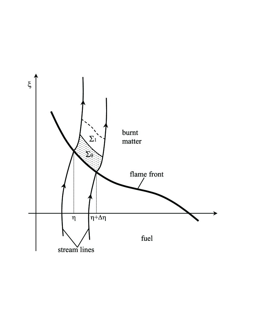
Figure 1: Kazakov, Physics of Fluids

Let us take a couple of stream lines crossing the flame front at points $(\eta,f(\eta))$ and $(\eta+\Delta\eta,f(\eta+\Delta\eta))$ (see Fig. 1). Consider the gas elements moving between these lines, which cross the front between the time instants $t=0$ and $t=\Delta t.$ During this time interval, these elements fill a space element $\Sigma_{0}$ adjacent to the flame front. For sufficiently small $\Delta\eta,\Delta t,$ the volume of $\Sigma_{0}$

$$\Delta s\approx\left|\begin{array}[]{cc}\Delta\eta&f^{\prime}\Delta\eta\\ w_{+}\Delta t&u_{+}\Delta t\\ \end{array}\right|=(u_{+}-f^{\prime}w_{+})\Delta\eta\Delta t=v^{n}_{+}N\Delta\eta\Delta t\,,$$

where

$$f^{\prime}\equiv\frac{df}{d\eta}\,,\quad N\equiv\sqrt{1+\left(f^{\prime}\right)^{2}}\ ;$$

the subscript“$+$” means that the corresponding quantity is evaluated just behind the flame front, i.e., for $\xi=f(\eta)+0,$ and $v^{n}_{+}=v_{i+}n_{i}$ is the normal velocity of the burnt gas, $n_{i}$ being the unit vector normal to the flame front (pointing to the burnt matter). After another time interval of the same duration $\Delta t,$ the elements move to a space element $\Sigma_{1}$ adjacent to $\Sigma_{0}.$ Since the flow is incompressible, $\Sigma_{1}$ is of the same volume as $\Sigma_{0}.$ Continuing this, the space between the two stream lines turns out to be divided into an infinite sequence of $\Sigma$’s of the same volume, adjacent to each other. Thus, summing over all $\Delta\eta,$ the third term in Eq. (9) can be written as

$$-\frac{\varepsilon_{ik}}{2}\partial_{k}\int\limits_{F}dl~{}v^{n}_{+}\sigma_{+}K(\eta,\xi,\tilde{\eta})\,,$$ (10)

where $F$ denotes the flame front surface (the front line in our 2D case),

$$K(\eta,\xi,\tilde{\eta}) = \frac{1}{\pi}\lim\limits_{\Delta t\to 0}\sum\limits_{n=0}^{\infty}\ln\left\{(\eta-{\rm H}(\tilde{\eta},n\Delta t))^{2}+(\xi-\Xi(\tilde{\eta},n\Delta t))^{2}\right\}^{1/2}\Delta t$$ (11)

$$= \frac{1}{\pi}\int\limits_{0}^{+\infty}dt\ln\left\{(\eta-{\rm H}(\tilde{\eta},t))^{2}+(\xi-\Xi(\tilde{\eta},t))^{2}\right\}^{1/2},$$

and $({\rm H}(\tilde{\eta},t),\,\Xi(\tilde{\eta},t))$ trajectory of a particle crossing the point $(\tilde{\eta},f(\tilde{\eta}))$ at $t=0.$

Substituting expression (10) into Eq. (9) gives

$$v_{i} = \varepsilon_{ik}\partial_{k}\int\limits_{\Lambda}dl_{l}~{}\varepsilon_{lm}v_{m}\frac{\ln r}{2\pi}-\partial_{i}\int\limits_{\Lambda}dl_{k}~{}v_{k}\frac{\ln r}{2\pi}-\frac{\varepsilon_{ik}}{2}\partial_{k}\int\limits_{F}dl~{}v^{n}_{+}\sigma_{+}K(\eta,\xi,\tilde{\eta})\,.$$ (12)

This representation of the flow velocity downstream will be used in the next section to determine the structure of the vortex mode near the flame front.

III Structure of the vortex mode

To determine the flame front dynamics, it is sufficient to know the flow structure near the flame front. As to the flow upstream, it is described by Eqs. (5), (6) for all $\xi<f(\eta).$ Given the solution upstream, velocity components of the burnt gas at the flame front can be found from the jump conditions which express the mass and momentum conservation across the front. On the other hand, these components are required to be the boundary values (for $\xi=f(\eta)+0$) of the velocity field satisfying the flow equations. As was shown in the preceding section, the latter can be represented in the integral form, Eq. (12). Any velocity field can be arbitrarily decomposed into a potential ($v_{i}^{p}$) and vortex ($v_{i}^{v}$) modes:

$$v_{i}=v_{i}^{p}+v_{i}^{v}\,.$$

Our strategy below will be to use the integral representation to determine the near-the-front structure of the vortex mode described by the last term in Eq. (12). As to $v_{i}^{p},$ the condition of its potentiality, expressed in the form of a “dispersion relation” at the flame front, will eventually close the system of integro-differential equations at the front.

Equation (12) reveals the following important fact. Up to a potential, the value of the vortex mode at a given point $(\eta,\xi)$ of the flow downstream is determined by only one point in the range of integration over $(\tilde{\eta},t),$ namely that satisfying

$${\rm H}(\tilde{\eta},t)=\eta\,,\quad\Xi(\tilde{\eta},t)=\xi\,.$$ (13)

This is, of course, a simple consequence of the Thomson theorem underlying the above derivation of Eq. (12). It can be verified directly by calculating the curl of the right hand side of Eq. (12): contracting this equation with $\varepsilon_{im}\partial_{m},$ using $\varepsilon_{ik}\varepsilon_{im}=\delta_{km},$ and taking into account the relation

$$\triangle\ln r=2\pi\delta^{(2)}(\zeta-\tilde{\zeta})\,,$$ (14)

one finds

$$\frac{1}{2}\varepsilon_{im}\partial_{m}\varepsilon_{ik}\partial_{k}\int\limits_{F}dl~{}v^{n}_{+}\sigma_{+}(\tilde{\eta})K(\eta,\xi,\tilde{\eta})=\int\limits_{0}^{+\infty}dt\int\limits_{F}dl~{}v^{n}_{+}\sigma_{+}(\tilde{\eta})\delta(\eta-{\rm H}(\tilde{\eta},t))\delta(\xi-\Xi(\tilde{\eta},t))\,.$$ (15)

Since $\delta(x)=0$ for $x\neq 0,$ the product of $\delta$-functions picks the point (13) out of the whole range of integration in the right hand side of Eq. (15).

Now, let us take the observation point $(\xi,\eta)$ sufficiently close to the flame front, i.e., $\xi\approx f(\eta),$ [$\xi>f(\eta)$]. In view of what has just been said, the vortex component for such points is determined by a contribution coming from the integration over $\tilde{\eta},t$ near the flame front, which corresponds to small values of $t.$ Integration over all other $\tilde{\eta},t$ gives rise to a potential contribution.

The small $t$ contribution to the integral kernel $K(\eta,\xi,\tilde{\eta})$ can be calculated exactly. For such $t$’s, one can write

$${\rm H}(\tilde{\eta},t)\approx\tilde{\eta}+w_{+}(\tilde{\eta})t\,,\quad\Xi(\tilde{\eta},t)\approx f(\tilde{\eta})+u_{+}(\tilde{\eta})t\,.$$ (16)

Let the equality of two fields $\varphi_{1}(\eta,\xi),\,\varphi_{2}(\eta,\xi)$ up to a potential field be denoted as $\varphi_{1}\stackrel{{\scriptstyle\circ}}{{=}}\varphi_{2}.$ Then, substituting Eq. (16) into Eq. (11), and integrating gives

$$K(\eta,\xi,\tilde{\eta}) = \frac{1}{\pi}\int\limits_{0}^{+\infty}dt\ln\left\{(\eta-{\rm H}(\tilde{\eta},t))^{2}+(\xi-\Xi(\tilde{\eta},t))^{2}\right\}^{1/2}$$ (17)

$$\stackrel{{\scriptstyle\circ}}{{=}} \frac{1}{\pi}\int\limits_{0}^{t_{0}}dt\ln\left\{v_{+}^{2}t^{2}-2\bm{rv_{+}}t+r^{2}\right\}^{1/2}$$

$$= \frac{1}{\pi}\int\limits_{-\frac{\bm{rv_{+}}}{v_{+}}}^{v_{+}t_{0}-\frac{\bm{rv_{+}}}{v_{+}}}dt_{1}\ln\left\{t_{1}^{2}-\frac{(\bm{rv_{+}})^{2}}{v_{+}^{2}}+r^{2}\right\}^{1/2}$$

$$= \frac{1}{\pi v_{+}}\left[\sqrt{r^{2}-\frac{(\bm{rv_{+}})^{2}}{v_{+}^{2}}}\arctan\frac{t_{1}}{\sqrt{r^{2}-\frac{(\bm{rv_{+}})^{2}}{v_{+}^{2}}}}\right.$$

$$\left.-t_{1}+t_{1}\ln\left\{t_{1}^{2}-\frac{(\bm{rv_{+}})^{2}}{v_{+}^{2}}+r^{2}\right\}^{1/2}\right]_{-\frac{\bm{rv_{+}}}{v_{+}}}^{v_{+}t_{0}-\frac{\bm{rv_{+}}}{v_{+}}}\,.$$

Here $v_{+}$ denotes the absolute value of the velocity field at the flame front, and $t_{0}$ is assumed small enough to justify the approximate equations (16).

As we know, the only point in the range of integration over $\tilde{\eta},t$ that contributes to the vortex mode is the one satisfying Eq. (13) or, after integrating over $t,$

$$[\eta-\tilde{\eta}]u_{+}(\tilde{\eta})-[\xi-f(\tilde{\eta})]w_{+}(\tilde{\eta})=0\,.$$ (18)

The distance $r$ between this point and the point of observation tends to zero as the latter approaches to the flame front surface. Thus, taking $[\xi-f(\eta)]$ small enough, one can make the ratio $t_{0}/r$ as large as desired; therefore, the right hand side of Eq. (17) is $\stackrel{{\scriptstyle\circ}}{{=}}$

$$\frac{r}{\pi v_{+}}\left\{\sqrt{1-\left(\frac{\bm{rv_{+}}}{rv_{+}}\right)^{2}}\left[\frac{\pi}{2}+\arcsin\left(\frac{\bm{rv_{+}}}{rv_{+}}\right)\right]-\frac{\bm{rv_{+}}}{rv_{+}}+\frac{\bm{rv_{+}}}{rv_{+}}\ln r\right\}+{\rm TIC}\,,$$ (19)

where “TIC” stands for “Terms Independent of the Coordinates” $(\eta,\xi).$ Denoting

$$\Omega=\frac{\bm{rv_{+}}}{rv_{+}}\,,$$

we finally obtain the following expression for the integral kernel

$$K(\eta,\xi,\tilde{\eta})\stackrel{{\scriptstyle\circ}}{{=}}\frac{r}{\pi v_{+}}\left\{\sqrt{1-\Omega^{2}}\left(\frac{\pi}{2}+\arcsin\Omega\right)+\Omega\ln\frac{r}{e}\right\}+{\rm TIC}\,.$$

In order to find the vortex mode of the velocity according to Eq. (12) we need to calculate derivatives of $K.$ Using the relation

$$\frac{\partial\Omega}{\partial\zeta_{i}}=\frac{1}{r}\left(\frac{v_{i+}}{v_{+}}-\Omega\frac{r_{i}}{r}\right)\,,\qquad r_{i}=\zeta_{i}-\tilde{\zeta}_{i}\,,$$ (20)

one easily obtains

$$\frac{\partial K}{\partial\zeta_{i}}\stackrel{{\scriptstyle\circ}}{{=}}\frac{1}{\pi v_{+}}\left\{\left(\frac{r_{i}}{r}-\Omega\frac{v_{i+}}{v_{+}}\right)\frac{\pi/2+\arcsin\Omega}{\sqrt{1-\Omega^{2}}}+\frac{v_{i+}}{v_{+}}\ln r\right\}\,.$$ (21)

Equation (21) can be highly simplified. Consider the quantity

$$\Upsilon_{i}=\left(\frac{r_{i}}{r}-\Omega\frac{v_{i+}}{v_{+}}\right)\frac{\arcsin\Omega-\pi/2}{\sqrt{1-\Omega^{2}}}+\frac{v_{i+}}{v_{+}}\ln r\,.$$ (22)

Let us evaluate $\partial_{i}\Upsilon_{i}\,.$ First, we calculate

$$\frac{\partial}{\partial\zeta_{i}}\left(\frac{r_{i}}{r}-\Omega\frac{v_{i+}}{v_{+}}\right)=\left(\frac{\partial_{i}r_{i}}{r}-r_{i}\frac{r_{i}}{r^{3}}\right)-\frac{\partial\Omega}{\partial r_{i}}\frac{v_{i+}}{v_{+}}=\frac{\Omega^{2}}{r}\,,$$ (23)

$$\frac{\partial}{\partial\zeta_{i}}\left(\frac{v_{i+}}{v_{+}}\ln r\right)=\frac{v_{i+}}{v_{+}}\frac{r_{i}}{r^{2}}=\frac{\Omega}{r}\,.$$ (24)

Second, we note that the vector

$$\beta_{i}=\left(\frac{r_{i}}{r}-\Omega\frac{v_{i+}}{v_{+}}\right)\frac{1}{\sqrt{1-\Omega^{2}}}$$

satisfies

$$\beta_{i}\beta_{i}=1,\qquad\beta_{i}v_{i+}=0\,,$$

i.e., $\beta_{i}$ is the unit vector orthogonal to ${\bf v}_{+}\,.$ In addition to that, $\beta_{i}$ changes its sign at the point defined by Eq. (18). Therefore, the derivative of $\beta_{i},$ entering $\Upsilon,$ contains a term with the Dirac $\delta$-function. However, this term is multiplied by $(\arcsin\Omega-\pi/2)$ which turns into zero together with the argument of the $\delta$-function. Therefore, the product of the additional term with $(\arcsin\Omega-\pi/2)$ is to be set zero, in the sense of distributions. Thus, using Eqs. (20), (23), (24) one finds

$$\frac{\partial\Upsilon_{i}}{\partial\zeta_{i}}=\frac{\Omega^{2}}{r}\frac{\arcsin\Omega-\pi/2}{\sqrt{1-\Omega^{2}}}+\left(\frac{r_{i}}{r}-\Omega\frac{v_{i+}}{v_{+}}\right)\left[\frac{1}{1-\Omega^{2}}+\Omega\frac{\arcsin\Omega-\pi/2}{(1-\Omega^{2})^{3/2}}\right]\frac{\partial\Omega}{\partial\zeta_{i}}+\frac{\Omega}{r}\equiv 0\,.$$

We conclude that $\Upsilon_{i}$ gives rise to a pure potential. A similar calculation shows that also

$$\varepsilon_{ik}\frac{\partial\Upsilon_{i}}{\partial\zeta_{k}}\equiv 0\,.$$ (25)

Therefore, we can rewrite Eq. (21) as

$$\frac{\partial K}{\partial\zeta_{i}}\stackrel{{\scriptstyle\circ}}{{=}}\frac{1}{v_{+}}\left(\frac{r_{i}}{r}-\Omega\frac{v_{i+}}{v_{+}}\right)\frac{1}{\sqrt{1-\Omega^{2}}}=\frac{\beta_{i}}{v_{+}}\,.$$ (26)

Finally, substituting this result into Eq. (12), noting that the vector $\varepsilon_{ki}\beta_{k}$ is the unit vector parallel to $v_{i+}$ if $\varepsilon_{ik}r_{i}v_{k+}>0,$ and antiparallel in the opposite case, we obtain the following expression for the vortex component of the gas velocity downstream near the flame front

$$v^{v}_{i}=\int\limits_{F}dl~{}\chi(\varepsilon_{pq}r_{p}v_{q+})\frac{v^{n}_{+}\sigma_{+}v_{i+}}{2v^{2}_{+}}\,.$$ (27)

Having written the exact equality in Eq. (27) we take this equation as the definition of the vortex mode. As a useful check, it is verified in appendix A that the obtained expression for $v^{v}_{i}$ satisfies

$$\left(\partial u^{v}/\partial\eta-\partial w^{v}/\partial\xi\right)_{+}\equiv\sigma_{+}\,.$$

It remains only to make the following comment in connection with the obtained expression for the vortex mode. As is clear from its derivation, Eq. (27) is applicable to unbounded as well as bounded flames. In the former case, however, the improper integral on the right of this equation is undefined, because integration over the infinite “tails” of the flame front around the point satisfying Eq. (18) gives rise to a potential contribution which is formally divergent. In the case of periodic flames which are of our main concern (see the beginning of Sec. II.1) this complication can be easily overcome if we specify that the integral is to be understood as

$$\int\limits_{F}d\eta\cdots=\lim\limits_{\mathbb{N}\ni n\to\infty}\int\limits_{-2bn}^{+2bn}d\eta\cdots\,,$$ (28)

so that the contributions of the tails cancel each other exactly. We prefer to work with an infinite $\eta$-interval, rather than $\eta\in[-b,b],$ because of the reasons that will be clear in Sec. IV.1.1.

IV Closed description of stationary flames

After we have determined the near-the-front structure of the vortex component of the gas velocity downstream, we can write down a closed system of equations governing the stationary flame propagation. As was explained in the Introduction, the term “closed” means that these equations relate only quantities defined on the flame front surface, without any reference to the flow dynamics in the bulk. This system consists of the jump conditions for the velocity components at the front, and the so-called evolution equation that gives the local normal fuel velocity at the front as a function of the front curvature. These equations (except for the evolution equation) are consequences of the mass and momentum conservation across the flame front. In Sec. IV.1, we obtain a closed system in the most general form, without specifying the form of the jump conditions, and then apply it to the case of zero thickness flames in Sec. IV.2.1.

IV.1 General formulation

First of all, we need to find the “on-shell” expression for the vortex component, i.e. its limiting form for $\xi\to f(\eta)+0.$ For this purpose we note that in this limit, $\chi(\varepsilon_{ik}r_{i}v_{k+})\to\chi(\eta-\tilde{\eta}),$ therefore, Eq. (27) gives

$$v^{v}_{i+}=\int\limits_{F}dl~{}\chi(\eta-\tilde{\eta})\frac{v^{n}_{+}\sigma_{+}v_{i+}}{2v^{2}_{+}}\,.$$ (29)

Let us denote the jump $[v_{i+}(\eta)-v_{i-}(\eta)]$ of the gas velocity $v_{i}$ across the flame front as $[v_{i}].$ Here $v_{i\pm}(\eta)\equiv v_{i}(\eta,f(\eta)\pm 0).$ Then we can write

$$v_{i-}+[v_{i}]=v^{p}_{i+}+\int\limits_{F}dl~{}\chi(\eta-\tilde{\eta})\sigma_{+}\frac{(v^{n}_{-}+[v^{n}])(v_{i-}+[v_{i}])}{2(v_{-}^{2}+[v^{2}])}\,.$$ (30)

In every finite order of the asymptotic expansion with respect to the flame front thickness, the jumps $[v_{i}]$ (as well as $\sigma_{+}$) are quasi-local functionals of the fuel velocity at the flame front, and of the flame front shape (i.e., depend on their values and the values of their derivatives of finite order in a given point). Two equations (30), together with Eq. (6) and the evolution equation, $v^{n}_{-}=v^{n}_{-}(f),$ form a system of four equations for the five functions $v_{i-}(\eta),v^{p}_{i+}(\eta),$ and $f(\eta).$ To close this system, we need an equation expressing potentiality of the field $v^{p}_{i},$ to be derived in the next section.

IV.1.1 A dispersion relation for the potential mode

By the construction, divergence of the last term in Eq. (12), describing the vortex mode, is zero identically in the entire downstream region. It is not difficult to see that it retains this property after the number of simplifications we have made in the course of derivation of the final expression (27). Note, first of all, that any operating with the integral kernel $K(\eta,\xi,\tilde{\eta})$ itself before differentiation with respect to $\zeta_{i}$ cannot break this property. On the other hand, Eq. (25) shows that divergence of the only term, namely $\Upsilon_{i},$ that have been omitted after this differentiation is zero identically. In view of the equation ${\rm div}\,\bm{v}=0,$ one concludes that the potential mode of the velocity field, $\bm{v}^{p},$ satisfies ${\rm div}\,\bm{v}^{p}=0$ downstream, too. Equations ${\rm rot}\,\bm{v}^{p}=0,$ ${\rm div}\,\bm{v}^{p}=0$ allow us to introduce the potential, $\phi,$ and the stream function, $\psi,$ according to

$$u^{p}=\frac{\partial\phi}{\partial\xi}=\frac{\partial\psi}{\partial\eta}\,,\qquad w^{p}=\frac{\partial\phi}{\partial\eta}=-\frac{\partial\psi}{\partial\xi}\,.$$ (31)

These relations imply that the combination $\Phi=\psi+i\phi$ is an analytical function of the complex variable $z=\eta+i\xi,$ and therefore so is its derivative $d\Phi/dz\equiv\omega^{p}=u^{p}+iw^{p}.$ Then, using the Cauchy theorem, we can write

$$\omega^{p}(z)=\frac{1}{2\pi i}\oint\limits_{\Lambda}d\tilde{z}\frac{\omega^{p}(\tilde{z})}{\tilde{z}-z}\,,$$ (32)

where $z\in\Sigma,$ and it is assumed that $\tilde{z}$ runs $\Lambda$ counterclockwise. In the course of derivation of the expression (27) for the vortex mode, we have been systematically omitting potential contributions. By the construction, these contributions are proportional to the integral kernel of the Laplace operator [Cf. Eq. (12)], and therefore, they generally diverge logarithmically at infinity [as, for instance, the last term in the expression (22)]. Hence, the integral over the part $\Lambda\diagdown F$ of the boundary of $\Sigma$ in Eq. (32) is formally an infinite constant, while the improper integral over $F$ is undefined. To avoid appearance of such divergent integrals, we will work below with the velocity derivative $d\omega^{p}/dz,$ instead of $\omega^{p}.$ Then Eq. (32) is replaced by

$$\frac{d\omega^{p}}{dz}(z)=\frac{1}{2\pi i}\oint\limits_{\Lambda}\frac{d\tilde{z}}{\tilde{z}-z}\frac{d\omega^{p}}{dz}(\tilde{z})\,.$$ (33)

Let us show that this identity can be rewritten as a dispersion relation for $d\omega/dz$ taken at the flame front. For this purpose, let us choose the contour of integration consisting of a large semicircle of radius $R,$ its center being at the point $z_{0}=0+if(0),$ and of the part of the front $F,$ indented by the circle. Then in the limit $z\to F,$ Eq. (33) takes the form

$$\frac{d\omega^{p}}{dz}(z_{+})=\frac{1}{\pi i}\mathchoice{{\vbox{\hbox{$\textstyle-$}}\kern-4.86108pt}}{{\vbox{\hbox{$\scriptstyle-$}}\kern-3.25pt}}{{\vbox{\hbox{$\scriptscriptstyle-$}}\kern-2.29166pt}}{{\vbox{\hbox{$\scriptscriptstyle-$}}\kern-1.875pt}}\!\int\limits_{F}\frac{d\tilde{z}}{\tilde{z}-z_{+}}\frac{d\omega^{p}}{dz}(\tilde{z})+\frac{1}{\pi}\int\limits_{0}^{\pi}d\varphi\lim\limits_{R\to\infty}\frac{d\omega^{p}}{dz}\left(Re^{i\varphi}\right)\,.$$ (34)

Our choice of the contour implies that the first integral on the right hand side of this equation is understood as

$$\int\limits_{F}d\tilde{z}\cdots=\lim\limits_{\mathbb{N}\ni n\to\infty}\int\limits_{z_{0}-2bn}^{z_{0}+2bn}d\tilde{z}\cdots\,.$$ (35)

According to what has been said about behavior of the potential mode at infinity,

$$\frac{d\omega^{p}}{dz}\left(Re^{i\varphi}\right)\to 0\quad{\rm as}\quad R\to\infty\quad{\rm for\ \ all}\quad\varphi\in(0,\pi).$$

Next, differentiating Eq. (29) with respect to $\eta,$ taking into account the relation

$$\frac{d\chi(x)}{dx}=2\delta(x)\,,$$ (36)

and performing the $\tilde{\eta}$-integration yields

$$\left(v^{v}_{i+}\right)^{\prime}=\frac{Nv^{n}_{+}\sigma_{+}v_{i+}}{v^{2}_{+}}\,.$$ (37)

On the other hand, one can write, in view of analyticity of $\omega^{p},$

$$\left(\omega^{p}_{+}\right)^{\prime}=\left(\frac{\partial\omega^{p}}{\partial\eta}\right)_{+}+f^{\prime}\left(\frac{\partial\omega^{p}}{\partial\xi}\right)_{+}=\left(1+if^{\prime}\right)\left(\frac{d\omega^{p}}{dz}\right)_{+}\,,$$

or,

$$\left(\frac{d\omega^{p}}{dz}\right)_{+}=\frac{1}{\left(1+if^{\prime}\right)}\left[\left(\omega_{+}\right)^{\prime}-\frac{Nv^{n}_{+}\sigma_{+}\omega_{+}}{v^{2}_{+}}\right]\,,\qquad\omega=u+iw\,.$$

The right hand side of this equation is explicitly periodic. Hence, the first integral in Eq. (34) is well-defined by the rule (35), so this equation becomes

$$\left(\frac{d\omega^{p}}{dz}\right)_{+}=\frac{1}{\pi i}\mathchoice{{\vbox{\hbox{$\textstyle-$}}\kern-4.86108pt}}{{\vbox{\hbox{$\scriptstyle-$}}\kern-3.25pt}}{{\vbox{\hbox{$\scriptscriptstyle-$}}\kern-2.29166pt}}{{\vbox{\hbox{$\scriptscriptstyle-$}}\kern-1.875pt}}\!\int\limits_{F}\frac{d\tilde{z}}{\tilde{z}-z_{+}}\left(\frac{d\omega^{p}}{dz}\right)_{+}\,.$$ (38)

A relation similar to Eq. (38) can be written for the gas velocity upstream:

$$\left(\frac{d\omega}{dz}\right)_{-}=-\frac{1}{\pi i}\mathchoice{{\vbox{\hbox{$\textstyle-$}}\kern-4.86108pt}}{{\vbox{\hbox{$\scriptstyle-$}}\kern-3.25pt}}{{\vbox{\hbox{$\scriptscriptstyle-$}}\kern-2.29166pt}}{{\vbox{\hbox{$\scriptscriptstyle-$}}\kern-1.875pt}}\!\int\limits_{F}\frac{d\tilde{z}}{\tilde{z}-z_{-}}\left(\frac{d\omega}{dz}\right)_{-}\,.$$ (39)

We have avoided appearance of potentially divergent quantities in the dispersion relation for the gas flow downstream at the cost of increasing its differential order by one$.^{13}$ Otherwise, we would have had to carry out all intermediate calculations for a finite domain $\Sigma,$ and to require all divergences to cancel in the final equation for the flame front position in the limit of infinite front length. In both cases, the finite constant in this equation (an integration constant in the first case, or a finite remainder after the cancellation in the second) is fixed by the normalization condition

$$V=\frac{1}{2b}\int\limits_{-b}^{+b}d\eta~{}N\,.$$ (40)

IV.1.2 The integro-differential relation between $\omega_{-}$ and $f.$

We are now in a position to write down the main integro-differential equation relating the values of the gas velocities at the flame front with the flame front position. To this end, we first differentiate Eq. (30) with respect to $\eta$ doing the integral as before, and rewrite the result in the complex form:

$$\left(\omega_{-}\right)^{\prime}+[\omega]^{\prime}=\left(\omega^{p}_{+}\right)^{\prime}+N\sigma_{+}\frac{(v^{n}_{-}+[v^{n}])(\omega_{-}+[\omega])}{(v_{-}^{2}+[v^{2}])}\,.$$ (41)

Acting on this equation by the operator

$$\left(1+if^{\prime}\right)\left(1-\frac{1}{\pi i}\mathchoice{{\vbox{\hbox{$\textstyle-$}}\kern-4.86108pt}}{{\vbox{\hbox{$\scriptstyle-$}}\kern-3.25pt}}{{\vbox{\hbox{$\scriptscriptstyle-$}}\kern-2.29166pt}}{{\vbox{\hbox{$\scriptscriptstyle-$}}\kern-1.875pt}}\!\int\limits_{F}\frac{d\tilde{z}}{\tilde{z}-z_{+}}\right)\left(1+if^{\prime}\right)^{-1}\,,$$

taking into account Eqs. (38), (39), and the relations

$$\left(\omega^{p}_{+}\right)^{\prime}=\left(1+if^{\prime}\right)\left(\frac{d\omega^{p}}{dz}\right)_{+}\,,\qquad\left(\omega_{-}\right)^{\prime}=\left(1+if^{\prime}\right)\left(\frac{d\omega}{dz}\right)_{-}$$

gives

$$2\left(\omega_{-}\right)^{\prime}+\left(1+i\hat{\mathcal{H}}\right)\left\{[\omega]^{\prime}-N\sigma_{+}\frac{(v^{n}_{-}+[v^{n}])(\omega_{-}+[\omega])}{(v_{-}^{2}+[v^{2}])}\right\}=0\,,$$ (42)

where

$$\hat{\mathcal{H}}=\frac{1+if^{\prime}}{\pi}\mathchoice{{\vbox{\hbox{$\textstyle-$}}\kern-4.86108pt}}{{\vbox{\hbox{$\scriptstyle-$}}\kern-3.25pt}}{{\vbox{\hbox{$\scriptscriptstyle-$}}\kern-2.29166pt}}{{\vbox{\hbox{$\scriptscriptstyle-$}}\kern-1.875pt}}\!\int\limits_{F}\frac{d\tilde{\eta}}{\tilde{z}-z_{+}}\,.$$

Written longhand, the action of the operator $\hat{\mathcal{H}}$ on a function $a(\eta)$ is

$$\left(\hat{\mathcal{H}}a\right)(\eta)=\frac{1+if^{\prime}(\eta)}{\pi}~{}\mathchoice{{\vbox{\hbox{$\textstyle-$}}\kern-4.86108pt}}{{\vbox{\hbox{$\scriptstyle-$}}\kern-3.25pt}}{{\vbox{\hbox{$\scriptscriptstyle-$}}\kern-2.29166pt}}{{\vbox{\hbox{$\scriptscriptstyle-$}}\kern-1.875pt}}\!\int\limits_{-\infty}^{+\infty}d\tilde{\eta}~{}\frac{a(\tilde{\eta})}{\tilde{\eta}-\eta+i[f(\tilde{\eta})-f(\eta)]}\,.$$ (43)

$\hat{\mathcal{H}}$ has properties similar to the Hilbert operator $\hat{H}.$ In particular, it is shown in appendix B.1 that

$$\hat{\mathcal{H}}^{2}=-1\,.$$ (44)

In terms of $\hat{\mathcal{H}},$ $\omega_{-},$ the dispersion relation (39) takes a more compact form

$$\left(1-i\hat{\mathcal{H}}\right)\left(\omega_{-}\right)^{\prime}=0\,.$$ (45)

In view of the property (44), this relation is fulfilled by any $\omega_{-}$ satisfying Eq. (42).

Equation (42) is the main integro-differential relation between the fuel velocity at the flame front, and the flame front position. It can also be rewritten in terms of $\omega_{+}$ as

$$2\left(\omega_{+}\right)^{\prime}-\left\{[\omega]^{\prime}+N\sigma_{+}\frac{v^{n}_{+}\omega_{+}}{v_{+}^{2}}\right\}+i\hat{\mathcal{H}}\left\{[\omega]^{\prime}-N\sigma_{+}\frac{v^{n}_{+}\omega_{+}}{v_{+}^{2}}\right\}=0\,.$$ (46)

Together with the jump conditions and the evolution equation which has the general form

$$v^{n}_{-}=1+S(u_{-},w_{-},f^{\prime})\,,$$ (47)

where $S$ is a quasi-local functional of its arguments, proportional to the flame front thickness, Eq. (42) provides a closed description of stationary flames.

IV.2 Equation (42) in lowest orders of the $\varepsilon$-expansion

In this section, the general results obtained in the preceding section will be applied to thin flames in the first two orders of the asymptotic expansion with respect to the flame front thickness $\varepsilon=L_{\rm f}/R.$

IV.2.1 Zero-thickness flames

For zero-thickness flames, the jump conditions for the velocity components have the form

$$[u] = \frac{\theta-1}{N}\ ,$$ (48)

$$[w] = -f^{\prime}\frac{\theta-1}{N}\,,$$ (49)

and hence,

$$[\omega] = (\theta-1)\frac{1-if^{\prime}}{N}\ ,$$ (50)

while the evolution equation

$$v^{n}_{-}=1\,.$$ (51)

We see that the jumps are velocity-independent, and $S\equiv 0.$ Also, it follows from these equations that

$$[v^{n}]=\theta-1\,,\quad[v^{2}]=\theta^{2}-1\,.$$

It remains only to calculate the value of the vorticity at the flame front, as a function of the fuel velocity. This can be done² directly using the flow equations (2),(3). With the help of Eqs. (5.32) and (6.15) of Ref. 2, the jump of the vorticity across the flame front can be written, in the 2D stationary case, as

$$[\sigma]=-\frac{\theta-1}{\theta N}\left(\hat{D}w_{-}+f^{\prime}\hat{D}u_{-}+\frac{1}{N}\hat{D}f^{\prime}\right),$$ (52)

where

$$\hat{D}\equiv\left(w_{-}+\frac{f^{\prime}}{N}\right)\frac{d}{d\eta}\,.$$ (53)

Differentiating the evolution equation written in the form

$$u_{-}-f^{\prime}w_{-}=N\,,$$ (54)

and writing Eq. (52) longhand, expression in the brackets can be considerably simplified

$$\hat{D}w_{-}+f^{\prime}\hat{D}u_{-}+\frac{1}{N}\hat{D}f^{\prime}\equiv w_{-}^{\prime}w_{-}+\frac{(f^{\prime}w_{-})^{\prime}}{N}+\frac{(f^{\prime})^{2}u_{-}^{\prime}}{N}+f^{\prime}u_{-}^{\prime}w_{-}+\frac{N^{\prime}}{N}$$

$$=\frac{(w_{-}^{2})^{\prime}}{2}+\frac{(u_{-}-N)^{\prime}}{N}+\frac{(N^{2}-1)u_{-}^{\prime}}{N}+u_{-}^{\prime}(u_{-}-N)+\frac{N^{\prime}}{N}=u_{-}^{\prime}u_{-}+w_{-}^{\prime}w_{-}\,.$$ (55)

Since the flow is potential upstream, we obtain the following expression for the vorticity just behind the flame front¹⁴

$$\sigma_{+}=-\frac{\theta-1}{\theta N}(u_{-}^{\prime}u_{-}+w_{-}^{\prime}w_{-})\,.$$ (56)

Substituting these expressions into Eq. (42) yields

$$\left(\omega_{-}\right)^{\prime}+\frac{\theta-1}{2}\left(1+i\hat{\mathcal{H}}\right)\left\{\left(\frac{1-if^{\prime}}{N}\right)^{\prime}+\frac{1}{2}\left(\omega_{-}+(\theta-1)\frac{1-if^{\prime}}{N}\right)\left[\ln(|\omega_{-}|^{2}+\theta^{2}-1)\right]^{\prime}\right\} \hskip-11.38092pt=0\,.$$

Equations (54) and (IV.2.1) provide the closed description of stationary zero-thickness flames in the most convenient form. Account of the heat conduction – species diffusion processes inside the thin flame front changes the right hand side of this equation to $O(\varepsilon).$ This modification will be considered in the next section.

IV.2.2 Account of the transport processes in the linear approximation

An equation relating $\omega_{-}$ with $f$ can be obtained also in the case of flames of nonzero thickness following the lines of the above derivation of Eq. (IV.2.1). For instance, in the first order in the flame front thickness $\varepsilon,$ one has to use in the general Eq. (42) the jump conditions and the evolution equation derived in Ref. 2. The resulting equation turns out to be much more complicated than Eq. (IV.2.1). However, the main purpose of taking into account the inner structure of the flame front is to provide a short wavelength cutoff for unstable flame perturbations, which is necessary for the very existence of stationary configurations of curved flames. On the other hand, for many purposes it is sufficient to consider the transport processes in the linear approximation, while full account of the nonlinear coupling of these processes to flame hydrodynamics is of minor importance in practice. Therefore, we can generalize Eq. (IV.2.1) to the case of flames of nonzero thickness almost without calculation using the results of the linear theory of flame front instability. In the linear approximation, $\omega_{-}=1,$ hence, the left hand side of Eq. (IV.2.1) reduces to

$$\frac{\theta-1}{2}\left(\hat{H}-i\right)f^{\prime\prime}\,.$$

On the other hand, omitting the time derivatives in the linear equation³ describing evolution of the front perturbations gives formally

$$\hat{H}f^{\prime}=\frac{\lambda_{c}}{2\pi}f^{\prime\prime}\,,$$

where $\lambda_{c}=L_{c}/R=O(\varepsilon)$ is the dimensionless cutoff wavelength. We conclude that the desired generalization of Eq. (IV.2.1) reads¹⁵

$$\left(\omega_{-}\right)^{\prime}+\frac{\theta-1}{2}\left(1+i\hat{\mathcal{H}}\right)\left\{\left(\frac{1-if^{\prime}}{N}\right)^{\prime}+\frac{1}{2}\left(\omega_{-}+(\theta-1)\frac{1-if^{\prime}}{N}\right)\left[\ln(|\omega_{-}|^{2}+\theta^{2}-1)\right]^{\prime}\right\}$$

$$=\frac{\theta-1}{2}\frac{\lambda_{c}}{2\pi}\left(1+i\hat{\mathcal{H}}\right)f^{\prime\prime\prime}\,.$$ (58)

Equivalently, the main system of equations can be rewritten in terms of $w_{+},u_{+}:$

$$\left(\omega_{+}\right)^{\prime}+\frac{\theta-1}{2}\left(-1+i\hat{\mathcal{H}}\right)\left(\frac{1-if^{\prime}}{N}\right)^{\prime}+\frac{\theta-1}{2}\left(1+i\hat{\mathcal{H}}\right)\left(\frac{\omega_{+}|\omega_{+}|^{\prime}}{|\omega_{+}|}-\frac{\lambda_{c}}{2\pi}f^{\prime\prime\prime}\right)=0\,,$$ (59)

$$u_{+}-f^{\prime}w_{+}=\theta N\,.$$

We have written $\hat{\mathcal{H}}$ instead of $\hat{H}$ in the $\varepsilon$-terms in order to formally preserve the dispersion relation (45). However, it should be kept in mind that by the construction, the $\varepsilon$-term is to be treated linearized.

Most probably, Eq. (IV.2.2) can be solved in full generality only numerically. However, it admits analytical solutions in lowest orders of the asymptotic expansion for $\theta\to 1,$ considered below.

V The small $(\theta-1)$ expansion

Although our main concern in this paper is the non-perturbative description of flames with arbitrary $\theta,$ it is of some interest to apply the above results to the case of weak gas expansion. One reason is that this case allows considerable simplification of Eqs. (54), (IV.2.2) which can be reduced to a single equation for the flame position. Another is that this is a good place to illustrate the role of the relation (40) in our approach. The well-known subtle point of the analytical theory of nonlinear flame propagation is to ensure that the constant $V$ and the function $f(\eta),$ which play the role of the eigenvalue and the eigenfunction of the nonlinear equation for the front position, respectively, satisfy this obvious condition.

In the present formulation, this problem does not arise at all. To see this, it is sufficient to note that the constant $V$ does not appear at all either in Eq. (IV.2.2), or in the evolution equation (54). Therefore, Eq. (40) is to be considered simply as a relation that allows one to express the flame velocity through the constant of integration $C$ [Cf. discussion in the end of Sec. IV.1.1]. In lowest orders of the small $(\theta-1)$ expansion, this connection between $V$ and $C$ can be followed out in detail. It will be shown in Sec. V.1 that in the first post-Sivashinsky approximation, Eqs. (54), (IV.2.2) reduce to the Cambray-Joulin¹⁶ version of the well-known Sivashinsky-Clavin equation$.^{4}$ In Sec. V.2, an equation for the flame front position will be obtained in the second post-Sivashinsky approximation, which represents a corrected version of the equation obtained by Kazakov and Liberman^5-6 (called there the fourth order equation).

V.1 The first post-Sivashinsky approximation

V.1.1 Equation for the flame front position

The form of the $\varepsilon$-term in Eq. (IV.2.2) shows that the cutoff wavelength $\lambda_{c}\sim 1/\alpha,$ $\alpha\equiv\theta-1.$ This implies that $f^{\prime}=O(\alpha),$ and that differentiation of a flow variable with respect to $\eta$ increases its order by one. Furthermore, it follows from Eq. (54) that $u_{-}=1+O(\alpha^{2}),$ since $V=O(\alpha^{2}).$ Then Eq. (6) tells us that also $w_{-}=O(\alpha^{2}).$ To carry out expansion of Eq. (IV.2.2), we need also to find the asymptotic action of the operator $\hat{\mathcal{H}}.$ A general procedure of consistent asymptotic treatment of this operator is formulated in appendix B.2. At the third order in $\alpha,$ according to Eq. (93), $\hat{\mathcal{H}}$ acts on the expression in the curly brackets on the left hand side of Eq. (IV.2.2) as the Hilbert operator. Thus, within accuracy of the fourth order, Eq. (IV.2.2) can be rewritten as

$$\left(\omega_{-}\right)^{\prime}+\frac{\theta-1}{2}\left(1+i\hat{H}\right)\left(\frac{1-if^{\prime}}{N}+\frac{|\omega_{-}|^{2}}{2\theta}-\frac{\lambda_{c}}{2\pi}f^{\prime\prime}\right)^{\prime}=0\,.$$

Expanding the last term in this equation, noting that with the required accuracy $|\omega_{-}|^{2}$ in the parentheses can be taken to be

$$|\omega_{-}|^{2}=1+\left(f^{\prime}\right)^{2}\,,$$ (60)

and integrating gives

$$\omega_{-}-\frac{\theta-1}{2}\left(1+i\hat{H}\right)\left(if^{\prime}+\frac{\lambda_{c}}{2\pi}f^{\prime\prime}\right)=C\,,$$ (61)

where $C=C_{1}+iC_{2}$ is the constant of integration. Extracting the real and imaginary parts of this equation, we obtain

$$u_{-} - \frac{\theta-1}{2}\left(-\hat{H}f^{\prime}+\frac{\lambda_{c}}{2\pi}f^{\prime\prime}\right)=C_{1}\,,$$ (62)

$$w_{-} - \frac{\theta-1}{2}\left(f^{\prime}+\frac{\lambda_{c}}{2\pi}\hat{H}f^{\prime\prime}\right)=C_{2}\,.$$ (63)

Integrating Eq. (63) over $[-b,+b],$ and taking into account periodicity of the function $f(\eta)$ shows that $C_{2}=0,$ because

$$\int\limits_{-b}^{+b}d\eta~{}w_{-}(\eta)=0$$

in view of the definition (1). Next, multiplying Eq. (63) by $f^{\prime},$ subtracting it from Eq. (62), and using the evolution equation (54), we arrive at the single equation for the flame front position¹⁷

$$\frac{\theta}{2}\left(f^{\prime}\right)^{2}=\frac{\theta-1}{2}\left(-\hat{H}f^{\prime}+\frac{\lambda_{c}}{2\pi}f^{\prime\prime}\right)+C_{1}-1\,.$$ (64)

The constant $C_{1}$ can be expressed through the flame velocity $V$ using the normalization condition (40). Namely, integrating Eq. (64) over $[-b,+b],$ and applying this condition gives

$$\theta\left(V-1\right)=C_{1}-1\,,$$

thus bringing the third order equation to the form

$$-\theta W+\frac{\theta}{2}\left(f^{\prime}\right)^{2}=\frac{\theta-1}{2}\left(-\hat{H}f^{\prime}+\frac{\lambda_{c}}{2\pi}f^{\prime\prime}\right)\,,$$ (65)

where $W\equiv V-1$ is the flame velocity increase due to the front curvature. This equation exactly coincides with the stationary version of the corrected Sivashinsky-Clavin equation (obtained by setting $\phi_{t}=-W,$ and restoring the $\varepsilon$-term in Eq. (10) of Ref. 16).

V.1.2 Solution of the equation (65)

The third order equation (65) is of the same functional structure as the Sivashinsky equation$.^{1}$ Therefore, it can be solved analytically using the method of pole decomposition$.^{18,19}$ We look for a $2b$-periodic solution of Eq. (65) in the form

$$f(\eta)=A\sum_{k=1}^{2P}\ln\sin\left[\frac{\pi}{2b}(\eta-\eta_{k})\right].$$ (66)

The amplitude $A$ and the complex poles $\eta_{k},$ $k=1,...,2P$ are to be determined substituting this anzats into Eq. (65). Since the function $f(\eta)$ is real for real $\eta,$ the poles come in conjugate pairs; $P$ is the number of the pole pairs.

Using the formulas (see Refs. 18,19 for more detail)

$$\hat{H}f^{\prime}=-\frac{\pi A}{2b}\sum_{k=1}^{2P}\left\{1+i~{}{\rm sign}({\rm Im}~{}\eta_{k})\cot\left[\frac{\pi}{2b}(\eta-\eta_{k})\right]\right\},~{}{\rm sign}(x)\equiv\frac{x}{|x|}\,,$$

$$\cot x\cot y=-1+\cot(x-y)(\cot y-\cot x)\,,$$

it is easily verified that Eq. (65) is satisfied by $f(\eta)$ taken in the form of Eq. (66), provided that

$$A = -\frac{\lambda_{c}}{2\pi}\frac{\theta-1}{\theta}\,,$$

$$W = \frac{(\theta-1)^{2}}{2\theta^{2}}\frac{P\lambda_{c}}{2b}\left(1-\frac{P\lambda_{c}}{2b}\right),$$ (67)

and the poles $\eta_{k},$ $k=1,...,2P\,,$ satisfy the following set of equations

$$i~{}{\rm sign}({\rm Im}~{}\eta_{k})+\frac{\lambda_{c}}{2b}\sum\limits_{\genfrac{}{}{0.0pt}{}{m=1}{m\neq k}}^{2P}\cot\left[\frac{\pi}{2b}(\eta_{k}-\eta_{m})\right]=0,~{}k=1,...,2P\,.$$ (68)

It is seen from Eq. (V.1.2) that the found solution (66) is not unique: there is a number of solutions corresponding to different numbers $P$ of poles. To identify the physical ones, a stability analysis of the solutions is required which, of course, cannot be carried out in the framework of the stationary theory. However, as we have mentioned above, the functional structure of Eq. (65) is very similar to that of the stationary Sivashinsky equation. Under assumption that the non-stationary versions of these equations are also similar, the stability analysis performed in Ref. 20 will be carried over the present case. According to this analysis, for a given (sufficiently small) $b,$ there is only one stable solution. This solution is identified as that maximizing the flame velocity. In addition to that, the poles of the stable solution are required to be vertically aligned in the complex $\eta$-plane. For such a “coalescent” solution, a simple upper bound on the number of poles can be obtained from Eq. (68). Namely, for $k=k_{0}$ with $\eta_{k_{0}}$ uppermost, one has

$$1=\frac{\lambda_{c}}{2b}\sum\limits_{\genfrac{}{}{0.0pt}{}{m=1}{m\neq k_{0}}}^{2P}\coth\left[\frac{\pi}{2b}({\rm Im}~{}\eta_{k_{0}}-{\rm Im}~{}\eta_{m})\right]\geq\frac{\lambda_{c}}{2b}(2P-1).$$

(The equality holds, if ${\rm Im}~{}\eta_{k_{0}}=\infty$) Then Eq. (V.1.2) tells us that the maximum $W$ is reached for

$$P_{{\rm max}}={\rm Int}\left(\frac{b}{\lambda_{c}}+\frac{1}{2}\right),$$

${\rm Int}(x)$ denoting the integer part of $x.$ Thus, the flame velocity increase $W_{s}$ of the stable solution takes the form

$$W_{s}=4W_{{\rm max}}\frac{P_{{\rm max}}\lambda_{c}}{2b}\left(1-\frac{P_{{\rm max}}\lambda_{c}}{2b}\right),$$ (69)

where

$$W_{{\rm max}}=\frac{(\theta-1)^{2}}{8\theta^{2}}\,.$$ (70)

V.2 The second post-Sivashinsky approximation

Before going into details of derivation of the correct fourth-order equation, let us take a pause to identify the origin of the failure of equations derived in Ref. 6 to satisfy the condition (40). It is traced to the choice of the constant term in the decomposition Eq. $(19)^{\prime}$ of the potential mode²¹ of the downstream flow (the formulas cited from Ref. 6 are distinguished by the prime). In Ref. 6, this term is taken to be equal to $\theta V.$ It reappears later in the right hand side of Eq. $(39)^{\prime}$ which is an integral of the main Eq. $(40)^{\prime}$. It was proved⁶ that Eq. $(40)^{\prime}$ is valid up to terms of the order $\alpha^{6}.$ However, this does not mean that Eq. $(39)^{\prime}$ is valid up to terms of the order $\alpha^{5}.$ The point is that the value $\theta V$ of the constant term in the potential mode is accurate only up to $O(\alpha^{3})$-terms. In other words, the proper decomposition of $u_{p}$ should read

$$u_{p}=\theta V+\beta+\tilde{u}_{p}\,,\qquad\tilde{u}_{p}=\int\limits_{-\infty}^{+\infty}dk\tilde{u}_{k}\exp(-|k|\xi+ik\eta)\,,$$

where $\beta=O(\alpha^{3})$ is some constant, instead of Eq. $(19)^{\prime}.$ Correspondingly, Eq. $(39)^{\prime}$ is to be substituted by the following

$$\phi=-\hat{H}\ln\frac{\Omega}{\theta V+\beta}\,.$$

Since $\theta,V,\Omega$ are all $O(1),$ this implies that an additive constant of the order $O(\alpha^{3})$ is missing in Eq. $(39)^{\prime}.$ The value of the constant $\beta$ is fixed eventually by the condition (40). As in the preceding section, it can be expressed through $W$ explicitly by averaging the resulting equation for the flame front position. It is not difficult to verify that following this way, one obtains exactly Eq. (65) instead of Eq. $(70)^{\prime}.$

V.2.1 Equation for the flame front position

Turning to the derivation of the fourth order equation, we write

$$|\omega_{-}|^{2}=1+\frac{\left(f^{\prime}u_{-}+w_{-}\right)^{2}}{N^{2}}=1+\left(f^{\prime}\right)^{2}+2f^{\prime}w_{-}+O(\alpha^{4})\,,$$ (71)

instead of Eq. (60). Substituting this into Eq. (IV.2.2), using Eq. (91), and integrating yields

$$\omega_{-}+\frac{\theta-1}{2}\left(1+i\hat{H}\right)\left\{\frac{1-if^{\prime}}{N}+\frac{\left(f^{\prime}\right)^{2}+2f^{\prime}w_{-}}{2\theta}-\frac{\lambda_{c}}{2\pi}f^{\prime\prime}\right\}$$

$$-i~{}\frac{\theta-1}{2\pi}\mathchoice{{\vbox{\hbox{$\textstyle-$}}\kern-4.86108pt}}{{\vbox{\hbox{$\scriptstyle-$}}\kern-3.25pt}}{{\vbox{\hbox{$\scriptscriptstyle-$}}\kern-2.29166pt}}{{\vbox{\hbox{$\scriptscriptstyle-$}}\kern-1.875pt}}\!\int\limits_{-\infty}^{+\infty}\frac{d\bar{\eta}}{\bar{\eta}-\eta}f^{\prime\prime}(\bar{\eta})\left[f(\bar{\eta})-f(\eta)\right]=C\,,$$ (72)

which replaces Eq. (61). Next, substituting the third order result for $w_{-}$ in the curly brackets in this equation, one finds with the required accuracy

$$\omega_{-}-\frac{\theta-1}{2}\left(1+i\hat{H}\right)\left\{\frac{if^{\prime}}{N}+\frac{\lambda_{c}}{2\pi}f^{\prime\prime}\right\}-i~{}\frac{\theta-1}{2\pi}\mathchoice{{\vbox{\hbox{$\textstyle-$}}\kern-4.86108pt}}{{\vbox{\hbox{$\scriptstyle-$}}\kern-3.25pt}}{{\vbox{\hbox{$\scriptscriptstyle-$}}\kern-2.29166pt}}{{\vbox{\hbox{$\scriptscriptstyle-$}}\kern-1.875pt}}\!\int\limits_{-\infty}^{+\infty}\frac{d\bar{\eta}}{\bar{\eta}-\eta}f^{\prime\prime}(\bar{\eta})\left[f(\bar{\eta})-f(\eta)\right]=C\,.$$

When extracting the real and imaginary parts, one notes that the last term in the latter equation is purely imaginary, and hence it affects only the $w_{-}$ component of the fuel velocity. Since this term is of the fourth order, it can be omitted because $w_{-}$ is multiplied by $f^{\prime}$ in the evolution equation. Thus, we have

$$u_{-}+\frac{\theta-1}{2}\hat{H}\left(\frac{f^{\prime}}{N}\right)-\frac{\theta-1}{2}\frac{\lambda_{c}}{2\pi}f^{\prime\prime}=C_{1}\,,$$ (73)

while for $w_{-}$ one can still use the third order Eq. (63) (with $C_{2}=0$). Apart from the $\varepsilon$-terms which are treated here differently from Ref. 6, equation (73) is nothing but the expression Eq. $(64)^{\prime}$ for $\upsilon$ (the $\xi$-independent counterpart of $u,$ introduced in Ref. 6), in which the constant term is modified as discussed above. Substituting $u_{-},w_{-}$ from Eqs. (63), (73) into the evolution equation (54) gives

$$N-C_{1}=\frac{\theta-1}{2}\left\{-\left(f^{\prime}+\hat{H}\right)\left(\frac{f^{\prime}}{N}\right)+\frac{\lambda_{c}}{2\pi}f^{\prime\prime}\right\}\,.$$

Averaging this equation along the flame front as before, noting that $f^{\prime}(-\eta)=-f^{\prime}(\eta),$ as a consequence of Eq. (1), and applying the condition Eq. (40) one can express the constant $C_{1}$ through $W.$ Thus, we obtain

$$N-1-\theta W=\frac{\theta-1}{2}\left\{-\left(f^{\prime}+\hat{H}\right)\left(\frac{f^{\prime}}{N}\right)+\frac{\lambda_{c}}{2\pi}f^{\prime\prime}\right\}\,.$$ (74)

As in the case of the third order equations (65) and $(70)^{\prime},$ the fourth order equations (74) and $(73)^{\prime}$ coincide exactly upon differentiation. To see this, one has to expand the $N$-factors in Eq. (74), to linearize the $\varepsilon$-terms in Eq. $(73)^{\prime},$ and to take into account that in the course of derivation of this equation, the Sivashinsky equation was used to transform some of the nonlinear terms.

V.2.2 Solution of the equation (74)

Remarkably, Eq. (74) can be further simplified, and brought to the form similar to that of Eq. (65). This can be done by expressing the terms of the third and fourth orders in $f^{\prime},$ which appear upon expanding the $N$-factors, through the lower-order terms using the Sivashinsky equation. Namely, rewriting this equation as

$$\frac{\left(f^{\prime}\right)^{2}}{2}=W-\frac{\theta-1}{2}\hat{H}f^{\prime}+O(\varepsilon)\,,$$ (75)

and taking its square, the term $(f^{\prime})^{4}/8$ coming from the $N$ on the left of Eq. (74) is substituted by

$$\frac{1}{2}\left[W^{2}-W(\theta-1)\hat{H}f^{\prime}+\frac{(\theta-1)^{2}}{4}\left(\hat{H}f^{\prime}\right)^{2}\right]\,,$$

which is already of the second order in $f^{\prime}.$ The $\varepsilon$-terms have been omitted because we neglect all nonlinearities related to the transport processes. Next, multiplying Eq. (75) by $f^{\prime},$ and acting by the Hilbert operator, the term $\hat{H}(f^{\prime})^{3}/2$ appearing on the right of Eq. (74) upon expanding $\hat{H}(f^{\prime}/N)$ becomes

$$\hat{H}\frac{\left(f^{\prime}\right)^{3}}{2}=W\hat{H}f^{\prime}-\frac{\theta-1}{4}\left[\left(\hat{H}f^{\prime}\right)^{2}-\left(f^{\prime}\right)^{2}\right]\,,$$

where we have used the well-known identity

$$2\hat{H}\left(a\hat{H}a\right)=\left(\hat{H}a\right)^{2}-a^{2}\,.$$

After substitution of these expressions, Eq. (74) can be rewritten in the following form, within accuracy of the fourth order,

$$\frac{2\theta^{2}\left(f^{\prime}\right)^{2}}{(\theta+1)^{2}}-\left(\theta W+\frac{W^{2}}{2}\right)=\frac{\theta-1}{2}\left(-\hat{H}f^{\prime}+\frac{\lambda_{c}}{2\pi}f^{\prime\prime}\right)\,.$$ (76)

Proceeding as in Sec. V.1.2, we look for a periodic solution of Eq. (76) in the form Eq. (66), and find

$$A = -\frac{\lambda_{c}}{2\pi}\frac{\theta-1}{4\theta^{2}}(\theta+1)^{2}\,,$$

$$\theta W+\frac{W^{2}}{2} = \frac{(\theta^{2}-1)^{2}}{8\theta^{2}}\frac{P\lambda_{c}}{2b}\left(1-\frac{P\lambda_{c}}{2b}\right)\,,$$

while equations for the pole positions remain the same [see Eqs. (68)]. As before, we identify the stable solution as that maximizing the flame velocity. In particular, the maximum of the flame velocity increase for a given $\theta$ is

$$W_{\rm max}=-\theta+\sqrt{\theta^{2}+\frac{(\theta^{2}-1)^{2}}{16\theta^{2}}}\,\,.$$

Because of the factor $1/16,$ the second term under the square root represents a relatively small correction to the first even for values of $\theta$ not close to unity, so the above expression can be simplified to

$$W_{\rm max}=\frac{(\theta^{2}-1)^{2}}{32\theta^{3}}\,.$$ (77)

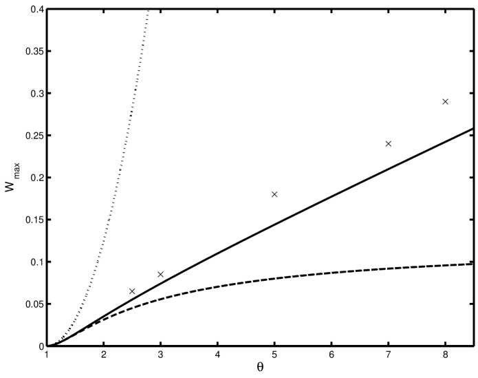
Figure 2: Kazakov, Physics of Fluids

Figure 2 compares the dependencies of the maximal flame velocity increase on the gas expansion coefficient, given by the Sivashinsky equation, and its corrections, Eqs. (65), (76), with the experimental data$.^{9,22}$ It is seen that the theoretical curve $W_{\rm max}(\theta)$ approaches the experimental marks as we pass from the Sivashinsky equation to the more accurate Eqs. (65), (76). However, one should remember that this improvement can be trusted only for sufficiently small values of $(\theta-1).$ For large values of the gas expansion coefficient it is rather a lucky accident. Only integration of the exact Eq. (IV.2.2) can give reliable results for the practically important values of $\theta\,.$

VI Discussion and conclusions

The results of Sec. IV solve the problem of closed description of stationary flames. The complex Eq. (42) determines the on-shell distribution of the fuel velocity as a functional of the flame front configuration in the most general form, while the evolution equation plays the role of a consistency condition which gives an equation for the front position itself. We have shown, furthermore, that in the case of zero-thickness flames, the main Eq. (42) takes the form (IV.2.1). This equation is universal in that any surface of discontinuity, propagating in an ideal incompressible fluid, is described by Eq. (IV.2.1) whatever internal structure of this discontinuity be. The latter shows itself in the $O(\varepsilon)$-corrections to this equation, where $\varepsilon$ is the relative thickness of the discontinuity. A simple comparison with the results of the linear theory has shown that the linear account of the heat conduction – species diffusion processes in the flame front modifies Eq. (IV.2.1) to Eq. (IV.2.2).

Next, some technical remarks are in order. It is difficult to say at the moment whether Eq. (IV.2.2) admits further simplification. What can be said, on the other hand, is that its analytical structure does not present serious problems for numerical integration. Indeed, the keystone of this structure is the integral operator $\hat{\mathcal{H}}.$ But its properties are much like those of the Hilbert operator $\hat{H}$ which is well-known how to deal with. From the theoretical point of view, Eq. (IV.2.2) is convenient for constructing various approximate descriptions of stationary flames. In particular, it is well suited for developing the small $(\theta-1)$ expansion which we have carried out in Sec. V. Specifically, it was verified in Sec. V.2 that at the second post-Sivashinsky approximation, the exact equations derived in the present paper reproduce the fourth order equation obtained in Ref. 6, up to an additive constant. This agrees completely with the main result of Sec. IIIB of Ref. 6, according to which Eq. $(40)^{\prime}$ correctly approximates the exact equation for the flame front position up to terms of the sixth order in $(\theta-1).$ The difference in the values of the additive constant was found in Sec. V.2 to be the result of an improper integration of Eq. $(40)^{\prime},$ namely of an incorrect separation of a constant term in the Fourier decomposition of the potential mode of the flow velocity downstream.

The results presented in this paper resolve the dilemma stated in the Introduction in the case of 2D stationary flames. Since in our considerations we have extensively used specifically 2D mathematical tools, the question of principle is whether the results of this paper can be carried over to the 3D case, and further to the general non-stationary case.

Appendix A Consistency check for Eq. (27)

After a lengthy calculation in Sec. III, we obtained the following simple expression for the vorticity mode near the flame front

$$v^{v}_{i}=\int\limits_{F}dl~{}\chi(\varepsilon_{pq}r_{p}v_{q+})\frac{v^{n}_{+}\sigma_{+}v_{i+}}{2v^{2}_{+}}\,.$$ (78)

As this important formula plays the central role in our investigation, a simple consistency check will be performed here, namely, we will verify that $v^{v}_{i}$ given by Eq. (78) satisfies

$$\left(\partial u^{v}/\partial\eta-\partial w^{v}/\partial\xi\right)_{+}\equiv\sigma_{+}\,.$$ (79)

Contracting Eq. (78) with $\varepsilon_{ki}\partial_{k},$ and using relation (36), one finds

$$\varepsilon_{ki}\partial_{k}v^{v}_{i}=\int\limits_{F}dl~{}\delta(\varepsilon_{pq}r_{p}v_{q+})\varepsilon_{ki}\varepsilon_{km}v_{m+}\frac{v^{n}_{+}\sigma_{+}v_{i+}}{v^{2}_{+}}=\int\limits_{F}dl~{}\delta(\varepsilon_{pq}r_{p}v_{q+})v^{n}_{+}\sigma_{+}\,.$$ (80)

The argument of the $\delta$-function turns into zero when the vectors $r_{i}$ and $v_{i+}$ are parallel. Near this point, one can write

$$\varepsilon_{pq}r_{p}v_{q+}\approx rv_{+}\phi\,,$$

where $\phi$ is the angle between the two vectors. On the other hand, the line element, $dl,$ near the same point can be written as

$$dl=\frac{r}{\sin\psi}d\phi=rd\phi\frac{v_{+}}{v^{n}_{+}}\,,$$

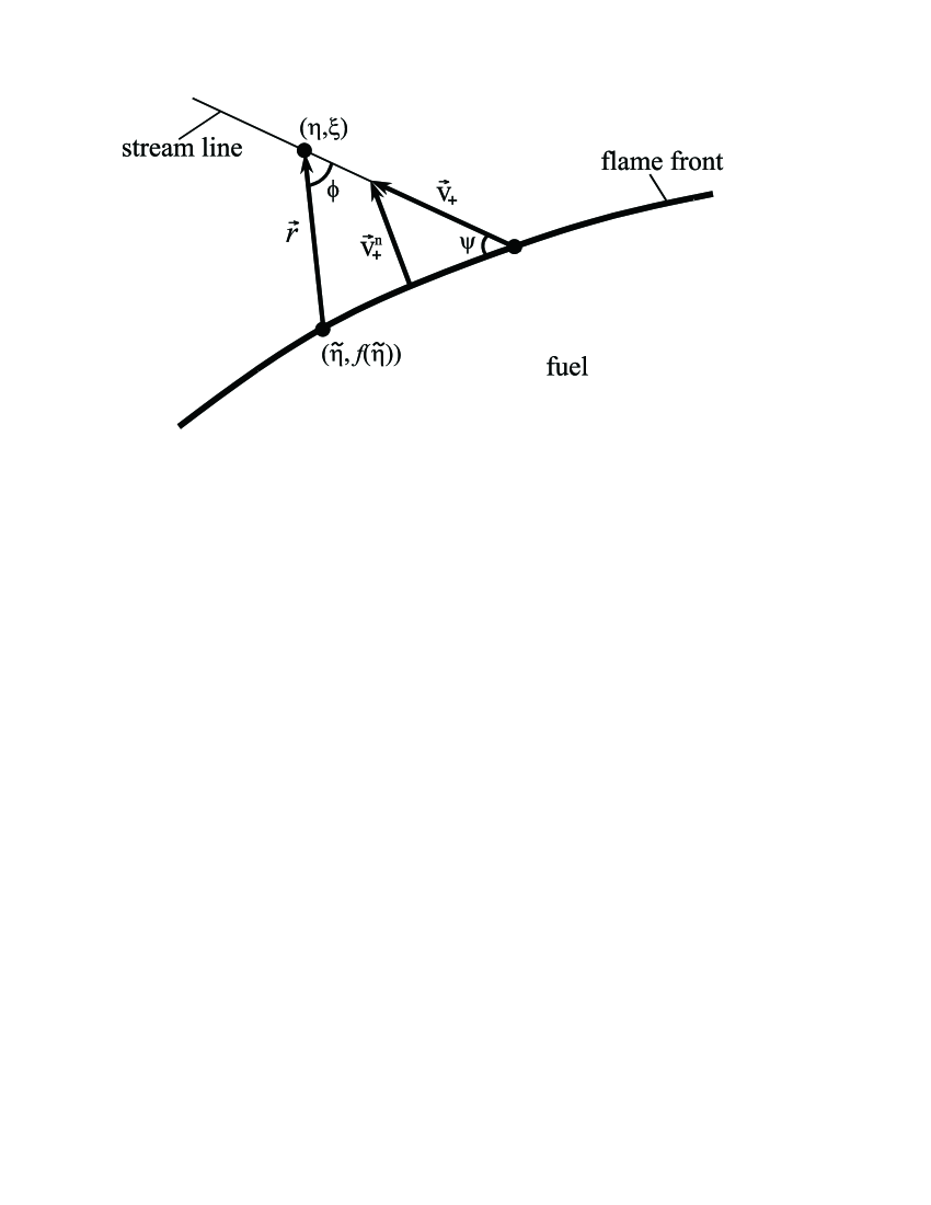
Figure 3: Kazakov, Physics of Fluids

as a simple geometric consideration shows, see Fig. 3.

Substituting these expressions into Eq. (80), and taking into account relation

$$\delta(\alpha x)=\frac{1}{|\alpha|}\delta(x)\,,$$

we finally arrive at the desired identity

$$\varepsilon_{ki}\partial_{k}v^{v}_{i}=\int\limits_{F}d\phi~{}\frac{rv_{+}}{v^{n}_{+}}~{}\delta(rv_{+}\phi)v^{n}_{+}\sigma_{+}=\int\limits_{F}d\phi~{}\delta(\phi)\sigma_{+}=\sigma_{+}\,.$$ (81)

It should be noted in this respect that the identity Eq. (79) is only a necessary condition imposed on the field $v^{v}_{i}.$ Playing the role of a “boundary condition” for the vortex mode, Eq. (79) is satisfied by infinitely many essentially different fields, i.e., fields which are not equal up to a potential. It is not difficult to verify, for instance, that the velocity field defined by

$$\tilde{v}^{v}_{i}=\int\limits_{F}dl~{}\chi(\varepsilon_{pq}r_{p}n_{q})\frac{\sigma_{+}n_{i}}{2}$$

also satisfies Eq. (79), and the difference $v^{v}_{i}-\tilde{v}^{v}_{i}$ is essentially non-zero.

By the construction of Sec. III, $v^{v}_{i}$ given by Eq. (78) is essentially the only field that satisfies the flow equations (2)-(3).

Appendix B Some properties of the operator $\hat{\mathcal{H}}$

B.1 Proof of the identity (44)

In the course of derivation of Eq. (42), we have introduced an operator $\hat{\mathcal{H}}$ defined on functionals of the flow variables by

$$\left(\hat{\mathcal{H}}a\right)(\eta)=\frac{1+if^{\prime}(\eta)}{\pi}~{}\mathchoice{{\vbox{\hbox{$\textstyle-$}}\kern-4.86108pt}}{{\vbox{\hbox{$\scriptstyle-$}}\kern-3.25pt}}{{\vbox{\hbox{$\scriptscriptstyle-$}}\kern-2.29166pt}}{{\vbox{\hbox{$\scriptscriptstyle-$}}\kern-1.875pt}}\!\int\limits_{-\infty}^{+\infty}d\tilde{\eta}~{}\frac{a(\tilde{\eta})}{\tilde{\eta}-\eta+i[f(\tilde{\eta})-f(\eta)]}\,,$$ (82)

and used repeatedly the following important identity it satisfies

$$\hat{\mathcal{H}}^{2}=-1\,.$$

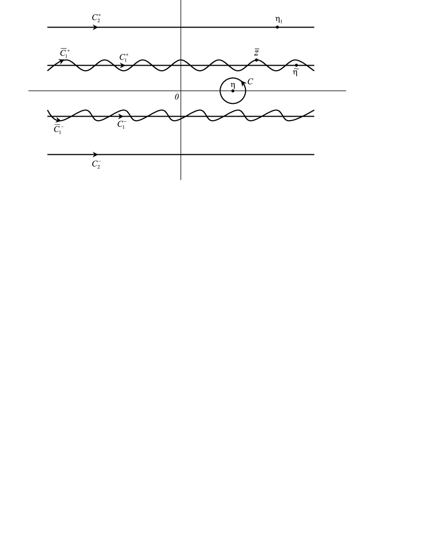
Figure 4: Kazakov, Physics of Fluids

To prove this identity, it is convenient to represent the right hand side of Eq. (82) as an integral over the contour $C_{1}=C_{1}^{-}\cup C_{1}^{+}$ in the complex $\tilde{\eta}$-plane, shown in Fig. 4

$$\left(\hat{\mathcal{H}}a\right)(\eta)=\frac{1+if^{\prime}(\eta)}{2\pi}~{}\int\limits_{C_{1}}d\tilde{\eta}~{}\frac{a(\tilde{\eta})}{\tilde{z}-z}\,,$$ (83)

where $z=\eta+if(\eta),$ $\tilde{z}=\tilde{\eta}+if(\tilde{\eta}),$ and $C_{1}$ is chosen such that all singularities of the integrand, except the pole at $\tilde{\eta}=\eta,$ remain above $C_{1}^{+},$ or below $C_{1}^{-}.$ Under our assumption about analytical properties of the functions involved [see discussion below Eq. (1)], such contour always exists. Now $\hat{\mathcal{H}}^{2}$ takes the form

$$\left(\hat{\mathcal{H}}^{2}a\right)(\eta)=\frac{1+if^{\prime}(\eta)}{4\pi^{2}}\int\limits_{C_{1}}\frac{d\tilde{z}}{\tilde{z}-z}\int\limits_{C_{2}}d\eta_{1}~{}\frac{a(\eta_{1})}{z_{1}-\tilde{z}}\,,\quad z_{1}=\eta_{1}+if(\eta_{1})\,,$$ (84)

where the contour $C_{2}=C_{2}^{-}\cup C_{2}^{+}$ of integration over $\eta_{1}$ comprises $C_{1}$ (see Fig. 4). Changing the order of integration in Eq. (84), using the formula

$$\int\frac{d\tilde{z}}{(\tilde{z}-z)(z_{1}-\tilde{z})}=\frac{1}{z_{1}-z}\ln\frac{\tilde{z}-z}{\tilde{z}-z_{1}}\ ,$$

and taking into account that the logarithm gives rise to a nonzero contribution only if the arguments of the functions $\tilde{z}-z$ and $\tilde{z}-z_{1}$ run in opposite directions when $\tilde{z}$ runs the contours $C_{1}^{\pm},$ we obtain

$$\frac{1+if^{\prime}(\eta)}{4\pi^{2}}\int\limits_{C_{1}}\frac{d\tilde{z}}{\tilde{z}-z}\int\limits_{C_{2}}d\eta_{1}~{}\frac{a(\eta_{1})}{z_{1}-\tilde{z}}=\frac{1+if^{\prime}(\eta)}{4\pi^{2}}\left(2\pi i\int\limits_{C_{2}^{-}}d\eta_{1}~{}\frac{a(\eta_{1})}{z_{1}-z}-2\pi i\int\limits_{C_{2}^{+}}d\eta_{1}~{}\frac{a(\eta_{1})}{z_{1}-z}\right)$$

$$=[1+if^{\prime}(\eta)]\frac{i}{2\pi}\int\limits_{C}d\eta_{1}~{}\frac{a(\eta_{1})}{z_{1}-z}=-[1+if^{\prime}(\eta)]\cdot{\rm res}\left.\frac{a(\eta_{1})}{(\eta_{1}-\eta)+i[f(\eta_{1})-f(\eta)]}\right|_{\eta_{1}=\eta}=-a(\eta)\,,$$

and thus

$$\left(\hat{\mathcal{H}}^{2}a\right)(\eta)=-a(\eta)$$

which was to be proved.

B.2 Asymptotic form of $\hat{\mathcal{H}}$ for $\theta\to 1$

It was shown in Sec. V that the exact equations derived in Sec. IV.1 constitute a general framework for perturbative treatment of flames within the small $(\theta-1)$-expansion. An important step of this program is the construction of an asymptotic expansion of the operator $\hat{\mathcal{H}}.$

Let us consider first an $\hat{\mathcal{H}}$-transform of a total derivative (this is the case we dealt with in Sec. V)

$$\left(\hat{\mathcal{H}}a^{\prime}\right)(\eta)=\frac{1+if^{\prime}(\eta)}{\pi}~{}\mathchoice{{\vbox{\hbox{$\textstyle-$}}\kern-4.86108pt}}{{\vbox{\hbox{$\scriptstyle-$}}\kern-3.25pt}}{{\vbox{\hbox{$\scriptscriptstyle-$}}\kern-2.29166pt}}{{\vbox{\hbox{$\scriptscriptstyle-$}}\kern-1.875pt}}\!\int\limits_{-\infty}^{+\infty}d\tilde{\eta}~{}\frac{a^{\prime}(\tilde{\eta})}{\tilde{\eta}-\eta+i[f(\tilde{\eta})-f(\eta)]}\,.$$ (85)

The aim of the subsequent transformations will be to develop an expansion of this integral in powers of $[f(\tilde{\eta})-f(\eta)]$ which is small for all $\tilde{\eta},$ rather than in powers of $(\tilde{\eta}-\eta).$ For this purpose we first rewrite it as an integral over the contour $C_{1}$ [Cf. Eq. (83)]

$$\left(\hat{\mathcal{H}}a^{\prime}\right)(\eta)=\frac{1+if^{\prime}(\eta)}{2\pi}~{}\int\limits_{C_{1}}\frac{da(\tilde{\eta})}{\tilde{z}-z}\,.$$ (86)

Integrating by parts then yields

$$\left(\hat{\mathcal{H}}a^{\prime}\right)(\eta)=\frac{1}{2\pi}\frac{d}{d\eta}~{}\int\limits_{\tilde{C}_{1}}d\tilde{z}~{}\frac{a(\tilde{\eta}(\tilde{z}))}{\tilde{z}-z}\,,$$ (87)

where $\tilde{C}_{1}$ denotes a contour in the complex $\tilde{z}$-plane, which is run by $\tilde{z}=\tilde{\eta}+if(\tilde{\eta})$ when $\tilde{\eta}$ runs $C_{1}.$ Next, let us make the following change of the integration variable in Eq. (87)

$$\tilde{z}\to\bar{z}=\tilde{z}-if(\eta)\,.$$

This gives

$$\left(\hat{\mathcal{H}}a^{\prime}\right)(\eta)=\frac{1}{2\pi}\frac{d}{d\eta}~{}\int\limits_{\bar{C}_{1}}d\bar{z}~{}\frac{a(\tilde{\eta}(\bar{z}))}{\bar{z}-\eta}\,,$$ (88)

where the contour $\bar{C}_{1}$ of $\bar{z}$-integration is obtained by a uniform vertical shift of $\tilde{C}_{1}$ by an amount $f(\eta).$ Note that $\bar{z}=\tilde{\eta}+i[f(\tilde{\eta})-f(\eta)]=\tilde{\eta}+O(\alpha).$ Hence, within the framework of the asymptotic expansion in $\alpha,$ $\bar{C}_{1}$ is to be considered as a small deformation of the initial contour $C_{1}.$ Taking $\alpha$ small enough we can always secure $C_{1}$ from crossing singularities of the integrand (including the pole $\tilde{\eta}=\eta$) under this deformation. Assuming this, we deform $\bar{C}_{1}$ back to the real axis, and obtain

$$\left(\hat{\mathcal{H}}a^{\prime}\right)(\eta)=\frac{1}{\pi}\frac{d}{d\eta}~{}\mathchoice{{\vbox{\hbox{$\textstyle-$}}\kern-4.86108pt}}{{\vbox{\hbox{$\scriptstyle-$}}\kern-3.25pt}}{{\vbox{\hbox{$\scriptscriptstyle-$}}\kern-2.29166pt}}{{\vbox{\hbox{$\scriptscriptstyle-$}}\kern-1.875pt}}\!\int\limits_{-\infty}^{+\infty}d\bar{\eta}~{}\frac{a(\tilde{\eta}(\bar{\eta}))}{\bar{\eta}-\eta}\,,$$ (89)

where $\tilde{\eta}(\bar{\eta})$ is a function of the real variable $\bar{\eta},$ defined by

$$\bar{\eta}=\tilde{\eta}+i[f(\tilde{\eta})-f(\eta)].$$

Resolving this relation with respect to $\tilde{\eta}$ in the form of a series

$$\tilde{\eta} = \bar{\eta}-i[f(\tilde{\eta})-f(\eta)]$$ (90)

$$= \bar{\eta}-i[f(\bar{\eta})-f(\eta)]-f^{\prime}(\bar{\eta})[f(\tilde{\eta})-f(\eta)]+\frac{i}{2}f^{\prime\prime}(\bar{\eta})[f(\tilde{\eta})-f(\eta)]^{2}+\dots$$

$$= \bar{\eta}-i[f(\bar{\eta})-f(\eta)]-f^{\prime}(\bar{\eta})[f(\bar{\eta})-f(\eta)]+i\left[f^{\prime}(\bar{\eta})\right]^{2}[f(\bar{\eta})-f(\eta)]$$

$$+\frac{i}{2}f^{\prime\prime}(\bar{\eta})[f(\bar{\eta})-f(\eta)]^{2}+\dots\,,$$

and substituting it into Eq. (89), we finally arrive at the following expansion of $\hat{\mathcal{H}}a^{\prime}$

$$\left(\hat{\mathcal{H}}a^{\prime}\right)(\eta) = \frac{1}{\pi}\frac{d}{d\eta}~{}\mathchoice{{\vbox{\hbox{$\textstyle-$}}\kern-4.86108pt}}{{\vbox{\hbox{$\scriptstyle-$}}\kern-3.25pt}}{{\vbox{\hbox{$\scriptscriptstyle-$}}\kern-2.29166pt}}{{\vbox{\hbox{$\scriptscriptstyle-$}}\kern-1.875pt}}\!\int\limits_{-\infty}^{+\infty}\frac{d\bar{\eta}}{\bar{\eta}-\eta}~{}\Bigl{\{}a(\bar{\eta})-ia^{\prime}(\bar{\eta})[f(\bar{\eta})-f(\eta)]-a^{\prime}(\bar{\eta})f^{\prime}(\bar{\eta})[f(\bar{\eta})-f(\eta)]$$ (91)

$$+ia^{\prime}(\bar{\eta})\left[f^{\prime}(\bar{\eta})\right]^{2}[f(\bar{\eta})-f(\eta)]-\frac{1}{2}a^{\prime\prime}(\bar{\eta})[f(\bar{\eta})-f(\eta)]^{2}+\dots\Bigr{\}}\,.$$

Since each term in the curly brackets in the integrand on the right of Eq. (91) is periodic, the corresponding improper integrals are well-defined by the rule (35).

Now it is straightforward to write down the result of asymptotic action of $\hat{\mathcal{H}}$ on a general $a(\eta).$ Namely, using $d/d\eta\hat{H}=\hat{H}d/d\eta$ in the first term in Eq. (91), and making the substitution $a^{\prime}(\eta)\to a(\eta)$ throughout this equation yields

$$\left(\hat{\mathcal{H}}a\right)(\eta) = \left(\hat{H}a\right)(\eta)+\frac{1}{\pi}\frac{d}{d\eta}~{}\mathchoice{{\vbox{\hbox{$\textstyle-$}}\kern-4.86108pt}}{{\vbox{\hbox{$\scriptstyle-$}}\kern-3.25pt}}{{\vbox{\hbox{$\scriptscriptstyle-$}}\kern-2.29166pt}}{{\vbox{\hbox{$\scriptscriptstyle-$}}\kern-1.875pt}}\!\int\limits_{-\infty}^{+\infty}\frac{d\bar{\eta}}{\bar{\eta}-\eta}~{}\Bigl{\{}-ia(\bar{\eta})[f(\bar{\eta})-f(\eta)]-a(\bar{\eta})f^{\prime}(\bar{\eta})[f(\bar{\eta})-f(\eta)]$$ (92)

$$+ia(\bar{\eta})\left[f^{\prime}(\bar{\eta})\right]^{2}[f(\bar{\eta})-f(\eta)]-\frac{1}{2}a^{\prime}(\bar{\eta})[f(\bar{\eta})-f(\eta)]^{2}+\dots\Bigr{\}}\,.$$

In the course of derivation of the third order equation in Sec. V, we found it necessary to determine the asymptotic action of $\hat{\mathcal{H}}$ on the curly bracket in the left hand side of Eq. (IV.2.2) taking into account $O(\alpha^{3})$ terms. In this case,

$$a^{\prime}=-if^{\prime\prime}+u_{-}^{\prime}=O(\alpha^{2})\,,$$

and therefore, it is sufficient to keep only the first term in the integrand of Eq. (91), which gives immediately

$$\left(\hat{\mathcal{H}}a^{\prime}\right)(\eta)=\left(\hat{H}a^{\prime}\right)(\eta)+O(\alpha^{4})\,.$$ (93)

¹G. I. Sivashinsky, “Nonlinear analysis of hydrodynamic instability in laminar flames,” Acta Astronaut. 4, 1177 (1977).

²M. Matalon and B. J. Matkowsky, “Flames as gasdynamic discontinuities,” J. Fluid Mech. 124, 239 (1982).

³P. Pelce and P. Clavin, “Influences of hydrodynamics and diffusion upon the stability limits of laminar premixed flames,” J. Fluid Mech. 124, 219 (1982).

⁴G. I. Sivashinsky and P. Clavin, “On the nonlinear theory of hydrodynamic instability in flames,” J. Physique 48, 193 (1987).

⁵K. A. Kazakov and M. A. Liberman, “Effect of vorticity production on the structure and velocity of curved flames,” Phys. Rev. Lett. 88, 064502 (2002).

⁶K. A. Kazakov and M. A. Liberman, “Nonlinear equation for curved stationary flames,” Phys. Fluids 14, 1166 (2002).

⁷L. D. Landau, “On the theory of slow combustion,” Acta Physicochimica URSS 19, 77 (1944).

⁸G. Darrieus, unpublished work presented at La Technique Moderne, and at Le Congr${\rm\grave{e}}$s de M${\rm\acute{e}}$canique Appliqu${\rm\acute{e}}$e, (1938) and (1945).

⁹V. V. Bychkov, S. M. Golberg, M. A. Liberman, and L. E. Eriksson, “Propagation of curved stationary flames in tubes,” Phys. Rev. E 54, 3713 (1996).

¹⁰We do consider zero-thickness flames in Sec. IV.2.1, but the only purpose of this consideration is to simplify treatment of the non-zero case.

¹¹Ya. B. Zel’dovich, A. G. Istratov, N. I. Kidin, and V. B. Librovich, “Flame propagation in tubes: hydrodynamics and stability,” Combust. Sci. and Tech. 24, 1 (1980).

¹²Indeed, the second term is a pure gradient, while the curl of the first term is proportional to $\Delta\ln r$ which is equal to zero everywhere in the bulk, Cf. Eq. (14).

¹³As to dispersion relation for the gas velocity upstream, it can be written directly in terms of $\omega$ itself, since the analog of Eq. (32) in this case is free of any divergences a priori, and gives in the limit $z\to F,$

$$\omega(z_{-})=-\frac{1}{\pi i}\mathchoice{{\vbox{\hbox{$\textstyle-$}}\kern-4.86108pt}}{{\vbox{\hbox{$\scriptstyle-$}}\kern-3.25pt}}{{\vbox{\hbox{$\scriptscriptstyle-$}}\kern-2.29166pt}}{{\vbox{\hbox{$\scriptscriptstyle-$}}\kern-1.875pt}}\!\int\limits_{F}\frac{d\tilde{z}}{\tilde{z}-z_{-}}\omega(\tilde{z})+V\,.$$

¹⁴Ya. B. Zel’dovich, G. I. Barenblatt, V. B. Librovich, and G. M. Makhviladze, The Mathematical theory of combustion and explosion (Consultants Bureau, New-York, 1985) pp. 466-470.

¹⁵Using this equation one should remember that the evolution equation still has the form (54) [all $\varepsilon$-contributions are already collected in the right hand side of Eq. (IV.2.2)].

¹⁶G. Joulin and P. Cambray, “On a tentative, approximate evolution equation for markedly wrinkled premixed flames,” Combust. Sci. and Tech. 81, 243 (1992).

¹⁷Another way to show that $C_{2}=0$ is to recall that no terms of the form $C_{2}f^{\prime}$ appear in the linear equation for the flame front position. However, we prefer the reasoning given in the text, because it avoids referring back to the linear theory.

¹⁸O. Thual, U. Frish, and M. Henon, “Application of pole decomposition to an equation governing the dynamics of wrinkled flames,” J. Phys. (France) 46, 1485 (1985).

¹⁹G. Joulin, “On the Zhdanov-Trubnikov equation for premixed flame stability,” J. Exp. Theor. Phys. 73, 234 (1991).

²⁰D. Vaynblat and M. Matalon, “Stability of pole solutions for planar propagating flames: I. Exact eigenvalues and eigenfunctions & II. Properties of eigenvalues and eigenfunctions with implication to flame stability,” SIAM J. Applied Math. 60, 679, 703 (2000).

²¹The same problem with the Sivashinsky-Clavin equation⁴ was shown¹⁶ to be of a similar origin.

²²M. A. Liberman et al., “Numerical studies of curved stationary flames in wide tubes,” Combust. Theory Modelling 7, 653 (2003).

Figure captions

Fig.1: Elementary decomposition of the flow downstream.

Fig.2: Dependence of the maximal flame velocity increase on the gas expansion coefficient, given by the Sivashinsky equation (dotted line), and its corrections – Eq. (65) (dashed line), and Eq. (76) (full line). The marks represent the results of numerical experiment^9,22 (accuracy of the experimental data is about $10\%$).

Fig.3: Near-the-front structure of the flow downstream. $\bm{v}^{n}_{+}=\bm{n}v^{n}_{+}$ is the normal component of the velocity. Since the observation point $(\eta,\xi)$ is close to the flame front, the stream line and the part of the front near this point can be considered straight.

Fig.4: Contours of integration in Eqs. (83) – (88)