Microwave traps for cold polar molecules

Abstract

We discuss the possibility of trapping polar molecules in the standing-wave electromagnetic field of a microwave resonant cavity. Such a trap has several novel features that make it very attractive for the development of ultracold molecule sources. Using commonly available technologies, microwave traps can be built with large depth (up to several Kelvin) and acceptance volume (up to several cm³), suitable for efficient loading with currently available sources of cold polar molecules. Unlike most previous traps for molecules, this technology can be used to confine the strong-field seeking absolute ground state of the molecule, in a free-space maximum of the microwave electric field. Such ground state molecules should be immune to inelastic collisional losses. We calculate elastic collision cross-sections for the trapped molecules, due to the electrical polarization of the molecules at the trap center, and find that they are extraordinarily large. Thus, molecules in a microwave trap should be very amenable to sympathetic and/or evaporative cooling. The combination of these properties seems to open a clear path to producing large samples of polar molecules at temperatures much lower than has been possible previously.

I Introduction

A growing interest has developed in extending the achievements of atomic cooling and trapping to molecules coldmolreviews , particularly polar molecules. The extremely large electric polarizability of such species enables access to strikingly new regimes and phenomena. For example, polar molecules subjected to strong electric fields have large laboratory-frame electric dipole moments, and thus can interact via the very strong, long-range dipole-dipole interaction. It has been argued that this can allow trapped polar molecules to be used as the qubits of a scalable quantum computer DeMilleQC . In addition, these interactions could make new types of highly-correlated quantum many-body states accessible, such as BCS-like superfluids ShlyapnikovBCS , supersolid and checkerboard states, two-dimensional Bose metals GoralpolarBEC , or effectively limited-dimensional gases manybodyrefs . Other applications include the possibility to study ultracold chemical reactions Dalgarnocoldchemistry , which might be controlled using electric fields Bohnfieldlinked . Finally, the increased spectroscopic precision associated with long observation times, combined with the enhanced sensitivity to certain types of perturbations, could allow the sensitivity of tests of fundamental symmetries to be increased to unprecedented levels MishaKreview .

At present, there remains no demonstrated technique for producing polar molecules with the very low temperatures $T$ ($T\lesssim 1$ mK) and high phase space densities required for most of these applications. Production of polar molecules at low translational temperatures, based on assembly from a sample of laser-cooled atoms, has recently been demonstrated using photoassociation at $T\sim 100\,\mu$K ourRbCspapers ; bagnatoKRb ; eylerKRb , and may soon be possible using Feshbach resonance-driven magneto-association at even lower temperatures Ingusciomixtures . Unfortunately, such methods produce molecular samples that, although translationally and rotationally cold, have their population in one or several highly-excited vibrational states. Methods are underway to drive part of the molecular ensemble to the rovibronic ground state, and to distill these ground state molecules from the sample. Such methods may eventually yield samples with the desired properties. However, this assembly method is unlikely to become widely useful because of its expense, complexity, and applicability to a very limited range of species.

Other groups have developed methods for direct cooling and/or slowing of molecules Doylebuffergastrap ; MeijerStarktrap ; Rempefilterguide ; Chandlerbilliard ; YeStarkslower . Samples of several molecular species have been produced at $T\sim 10-100$ mK, in all degrees of freedom (translational, vibrational, rotational), and the resulting molecules have been (or clearly could be) subsequently trapped. These direct-cooling methods have wide applicability and are simpler than the assembly approach. However, they require a new technological step to reach temperatures substantially lower than $T\sim 10$ mK. Collisional cooling of the trapped molecules (sympathetic and/or evaporative) appears to be the only viable technique for breaking through this temperature barrier.

Unfortunately, it seems that the prospects are either uncertain, or demonstrably poor, for further collisional cooling of molecules in most of the traps now employed. The essential problem is that these traps are based on static electromagnetic (EM) fields. Since static EM fields cannot have a maximum in free space, these traps hold only weak-field seeking molecules, which are by necessity in an internally excited state. Thus, in such traps there is always a channel for inelastic collisions, which can lead to loss of trapped molecules. The rotational degree of freedom of molecules can greatly enhance such inelastic loss mechanisms, relative to atoms; thus several authors have expressed pessimism about the prospects for collisional cooling of molecules in electrostatic traps Bohnpolarcollisions ; Kajitasemiclassical ; Kajitacolder as well as magnetostatic traps Bohnmagnetictrapcollisions . While there may be certain situations where the problems with collisional cooling in static traps can be avoided Kajitafermions , it seems unlikely that such traps could be used very generally for this purpose.

There have been two types of traps for strong-field seeking (ground state) molecules discussed previously in the literature. In the first of these, a centrifugal barrier associated with the molecules’ orbital angular momentum around the trap center (e.g., around a charged wire Starkwiretrap , or in a storage ring Meijerstoragering ) prevents the molecules from colliding with the electrodes where the strongest electric fields exist. Such traps are obviously not suitable for collisional cooling to very low temperatures. A more promising trap has recently been demonstrated, based on low frequency modulation of a static trap. The principle of such traps is similar to that of the Paul trap for charged particles RempePaultrap . However, with realistic technical parameters, such traps for strong-field seekers are typically both shallow (with trap depth $D\lesssim 10$ mK) and small (with volume $V\lesssim 10^{-3}$ cm³). These constraints will make it difficult to load large samples of polar molecules into such ”dipole Paul traps”, using currently available sources of precooled molecules.

In this paper we propose and discuss a new type of trap, based on the large low-frequency electric polarizability of polar molecules. In particular, we argue that it is viable to trap and collisionally cool molecules in the strong, high-frequency electric field of a microwave resonant cavity. Such a microwave trap has several notable advantages over the traps now employed for directly-cooled molecules, and may be very useful in the effort to further cool the samples of polar molecules now available. The advantages of the microwave trap include:

• The microwave field can trap molecules in their absolute ground state (a strong-field seeking state), at a free-space maximum of the high-frequency electric field. This in turn eliminates all concerns about two-body inelastic collisions leading to loss of molecules during evaporative or sympathetic cooling.

• With reasonable technical parameters, the microwave trap can have large depth $D$ ($D>1$ K) and volume $V$ ($V>1$ cm³), allowing it to be loaded easily from proven sources of directly-cooled molecules Doylebuffergastrap ; MeijerStarktrap ; Rempefilterguide ; Chandlerbilliard ; YeStarkslower . Note that optical dipole traps (which are similar in principle to the microwave trap) can also trap ground-state molecules, but optical traps are both much shallower and of much smaller volume than the microwave trap.

• An open trap geometry (using a Fabry-Perot microwave cavity) should allow easy overlap of the molecules with laser-cooled atoms. The microwave field will also act as a weak trap for the atoms. Thus sympathetic pre-cooling to temperatures well below 1 mK seems very promising in the microwave trap.

• Strong-field seeking states reside in the region of maximum electric field, where they are electrically polarized. The resulting dipole-dipole interaction results in huge elastic collision cross-sections ($\sigma$), which are desirable for evaporative cooling. This cross-section actually increases as the temperature of the molecules decreases ($\sigma\propto T^{-1/2}$) Kajitasemiclassical . Thus, with sufficiently high initial density, the prospects seem very favorable for bringing the trapped molecules to a regime of runaway evaporative cooling.

In the following sections we will outline the basic principle of the microwave trap, in terms of the energy shifts of molecules subjected to a microwave field; discuss realistic design parameters for an implementation of the trap; and finally, discuss collisions within the trap.

II Energy level shifts of polar molecules in a microwave field

The basic principle of the microwave trap is to take advantage of the AC Stark shift associated with low-frequency transitions arising from rotational (or inversion-doublet or Lambda/Omega doublet) structure in polar molecules. For the purposes of this paper, we confine the discussion to the effect of the microwave electric field on diatomic molecules with simple rigid rotor structure (e.g., in ${}^{1}\Sigma$ electronic states), although the ideas can be easily extended to molecules with more complex structure. In addition, we consider primarily the effect on the rotational ground state ($J=0$), although such traps can also be effective for other states under proper conditions. We assume the molecule is subject to a harmonically-varying electric field $\mbox{\boldmath$\mathcal{E}$}(t)=\textrm{Re}\{\mbox{\boldmath$\mathcal{E}$}_{0}e^{i\omega t}\}=\mathcal{E}_{0}\textrm{Re}\{\mbox{\boldmath$\epsilon$}e^{i\omega t}\}$, where $\epsilon$ is the complex unit vector indicating the polarization. Moreover, we assume that trap microwave angular frequency $\omega$ satisfies $\hbar\omega\lesssim B_{e}$, where $B_{e}$ is the rotational constant. [$B_{e}$ is defined such that the field-free energy $E(J)$ of the state with rotational quantum number $J$ is $E(J)=B_{e}J(J+1)$.] The response of polar molecules to such low-frequency electric fields is dominated by the coupling to nearby rotational levels; as such it is a good approximation to ignore the vibrational and electronic structure of the molecule. The Hamiltonian of the system is then $H=H_{0}+H^{\prime}$, where $H_{0}=B_{e}\mathbf{J}^{2}$, $H^{\prime}=-\mu\mathbf{n}\cdot\mbox{\boldmath$\mathcal{E}$}$, $\mu$ is the electric dipole moment in the molecule-fixed frame, and $\mathbf{n}$ is the operator indicating the unit vector along the molecular symmetry axis. The eigenstates of $H_{0}$ are defined by the quantum numbers $J$ and $m=\left\langle J_{z}\right\rangle$.

We have performed a general calculation of the AC Stark shift ${\Delta E}$ of the $J=0$ state, which determines the trap depth. Before describing this general calculation, however, it is instructive to consider the behavior of ${\Delta E}$ in some simple limiting cases. For low electric field strength ($\mu\mathcal{E}_{0}\ll B_{e}$), ${\Delta E}$ can be calculated from standard time-dependent perturbation theory. To second order,

$${\Delta E} = -\frac{1}{4}\sum\limits_{J^{\prime},m^{\prime}}\frac{\left|{\left\langle{J^{\prime},m^{\prime}}\right|H^{\prime}\left|{J=0,m=0}\right\rangle}\right|^{2}}{E(J^{\prime})-E(0)-\hbar\omega}$$ (1)

$$\;\;\;\;\;\;\;\;\;\;+\;\frac{\left|{\left\langle{J^{\prime},m^{\prime}}\right|H^{\prime}\left|{J=0,m=0}\right\rangle}\right|^{2}}{E(J^{\prime})-E(0)+\hbar\omega}$$

$$= -\frac{\mu^{2}\mathcal{E}_{2}^{2}}{4}\sum\limits_{m^{\prime}}\frac{\left|{\left\langle{1,m^{\prime}}\right|\mathbf{n}\cdot\mbox{\boldmath$\epsilon$}\left|{0,0}\right\rangle}\right|^{2}}{2B_{e}-\hbar\omega}$$

$$\;\;\;\;\;\;\;\;\;\;\;\;\;\;+\;\frac{\left|{\left\langle{1,m^{\prime}}\right|\mathbf{n}\cdot\mbox{\boldmath$\epsilon$}\left|{0,0}\right\rangle}\right|^{2}}{2B_{e}+\hbar\omega}$$

$$= \frac{\mu^{2}\mathcal{E}_{2}^{2}}{4}\sum\limits_{m^{\prime}}\frac{\left|{\left\langle{1,m^{\prime}}\right|\mathbf{n}\cdot\mbox{\boldmath$\epsilon$}\left|{0,0}\right\rangle}\right|^{2}}{\hbar\Delta}$$

$$\;\;\;\;\;\;\;\;\;\;\;+\;\frac{\left|{\left\langle{1,m^{\prime}}\right|\mathbf{n}\cdot\mbox{\boldmath$\epsilon$}\left|{0,0}\right\rangle}\right|^{2}}{\hbar\Delta-2\hbar\omega}$$

where we have used the fact that matrix elements of the form $\left\langle{J^{\prime},m^{\prime}}\right|H^{\prime}\left|{J,m}\right\rangle$ vanish unless $J^{\prime}=J\pm 1$ TownesandSchawlow , and we have defined the detuning $\Delta$ of the microwave field from the $J=0\leftrightarrow J=1$ resonance: $\Delta\equiv\omega-2B_{e}$. This perturbative expression makes clear some of the salient features of the microwave trap. In particular, it is evident that for red detuning ($\Delta<0$), ${\Delta E}<0$; thus in this case $J=0$ molecules are attracted to regions of strong microwave electric field. Moreover, ${\Delta E}$ (which will be the trap depth) can be enhanced by operating at small detuning.

The microwave trap is clearly similar to the more-familiar optical dipole trap, which is used commonly for laser-cooled atoms opticaldipoletraps . For optical traps, it is impractical to operate in the regime of small detuning $\hbar\left|{\Delta}\right|\lesssim\mu\mathcal{E}_{0}$, since in this case a high rate of spontaneous emission from the nearby, short-lived electronically excited state leads to rapid heating of the sample. The expression for the depth of an optical dipole trap is thus typically written in the perturbative limit as above. By contrast, the spontaneous-emission lifetimes of rotational states are much longer than typical trap lifetimes; thus heating by photon scattering cannot be troublesome in microwave traps. This makes it possible, in principle, to operate at arbitrarily small detunings, where trap depth is maximized.

It is also instructive to consider the limit of low frequency, $\hbar\omega\ll B_{e}$. Here, for a linearly-polarized field $\mbox{\boldmath$\epsilon$}=\hat{z}$, ${\Delta E}$ must be the same as the DC Stark shift ${\Delta E}_{DC}$ in an applied DC electric field $\mbox{\boldmath$\mathcal{E}$}_{DC}=\left({\mathcal{E}_{0}/\sqrt{2}}\right)\hat{z}$. (The factor of $1/\sqrt{2}$ arises from the fact that the molecule responds, on average, to the r.m.s. microwave field strength; this is in turn because the Stark effect is a second-order effect in the low-field limit.) Indeed, Eq.(1) reproduces the familiar perturbative expression for ${\Delta E}_{DC}$ in the limit $\omega\rightarrow 0$ TownesandSchawlow . A numerical calculation of DC Stark shifts in larger fields ($\mu\mathcal{E}_{DC}\gtrsim B_{e}$) is straightforward, and has been presented in, e.g., Ref. DeMilleQC . This calculation yields the result that ${\Delta E}_{DC}\sim-(\mu/2)\mathcal{E}_{DC}$ for large electric fields. This is in accord with a simple physical picture in which the large field almost completely polarizes the $J=0$ state, which then responds in the same way as a fixed electric dipole in an external electric field. From this picture, it can be anticipated that even for higher frequencies $\hbar\omega\sim B_{e}$, microwave traps should have similar shifts, ${\Delta E}\sim-(\mu/2)\mathcal{E}_{0}$, for moderately strong fields $\mu\mathcal{E}_{0}\gtrsim B_{e}$.

Neither of the limiting cases discussed so far is sufficient to describe the optimal conditions for the microwave trap. In order to obtain large trap depths it is necessary to have $\mu\mathcal{E}_{0}\gtrsim B_{e}$, so that the low-field limit does not apply. In addition, the desire to trap the molecules in a free-space maximum of $\mathcal{E}_{0}$ means that the dimensions of the trap must be at least as large as the microwave wavelength $\lambda=2\pi c/\omega$. For practical trap sizes, this requires $\hbar\omega\sim B_{e}$; this is preferable in any case, to maximize ${\Delta E}$ by operating at small detuning $\Delta$.

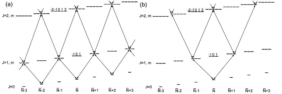
Figure 1: Dressed-state energy level diagrams for rotational states of a diatomic molecule subject to a microwave electric field. The indices at the bottom indicate the photon number $\bar{N}+n$, where $\bar{N}$ is the average number of photons in the field; the labels $J,m$ at the side indicate the rotational angular momentum and its $z$-projection, respectively. Arrows indicate $1^{st}$-order couplings between levels due to $H^{\prime}_{q}$; unterminated arrows couple to levels outside the range of the figure. The subset of the Hilbert space used for the calculations described in the main text consists of only levels connected to $\left|{\psi_{000}}\right\rangle=\left|{0,0}\right\rangle\left|{\bar{N}}\right\rangle$ with some number of arrows. For clarity, we have chosen $\hbar\omega=0.2B_{e}$ for this figure. (a) Linear polarization $\mbox{\boldmath$\epsilon$}=\hat{z}$. (b) Circular polarization $\mbox{\boldmath$\epsilon$}=(\hat{x}-i\hat{y})/\sqrt{2}$. Note that the linearly-polarized case contains many more states, and inevitably includes near-degeneracies at some values of $n$.

We have calculated ${\Delta E}$ for a more general range of $\omega$ and $\mathcal{E}_{0}$, using the dressed-state formalism CohenTannoudji . The classical-field Hamiltonian $H$ is replaced with its quantized-field analogue: $H_{q}=H_{0q}+H^{\prime}_{q}$, where

$$H_{0q}=B_{e}\mathbf{J}^{2}+\hbar\omega(\hat{N}-\bar{N})$$ (2)

and

$$H^{\prime}_{q}=-\mu\mathbf{n}\cdot\mbox{\boldmath$\mathcal{E}$}=-\mu\sqrt{\frac{\hbar\omega}{2\omega}{2\epsilon_{0}V}}\left[{(\mathbf{n}\cdot\mbox{\boldmath$\epsilon$}^{*})a^{{\dagger}}+(\mathbf{n}\cdot\mbox{\boldmath$\epsilon$})a}\right].$$ (3)

Here we have introduced the photon creation and destruction operators $a^{{\dagger}},a$, and the photon number operator $\hat{N}=a^{{\dagger}}a$. (The parameter $V$ refers to the volume of a fictitious box used to define the boundary conditions of the quantized electromagnetic field; as usual in such calculations, all relevant physical quantities are independent of $V$.) The energy scale is defined relative to the mean number of photons in the field, $\bar{N}=\frac{\mathcal{E}_{0}^{2}}{2}\frac{\epsilon_{0}V}{\hbar\omega}$. Throughout we are interested in strong fields, so that $\bar{N}\gg 1$. We use as basis states the molecule+field eigenstates of $H_{0q}$: $\left|{\psi_{Jmn}}\right\rangle=\left|{J,m}\right\rangle\left|{\bar{N}+n}\right\rangle$, where $\bar{N}+n$ is the dressed-state photon number. The diagonal matrix elements of $H_{q}$ are $\left\langle{\psi_{Jmn}}\right|H_{q}\left|{\psi_{Jmn}}\right\rangle=B_{e}J(J+1)+n\hbar\omega$. Off-diagonal matrix elements of the form $\left\langle{\psi_{J^{\prime}m^{\prime}n^{\prime}}}\right|H_{q}\left|{\psi_{Jmn}}\right\rangle$ vanish unless $J^{\prime}=J\pm 1$ and $n^{\prime}=n\pm 1$. Explicitly, using the approximation that $\sqrt{\bar{N}\pm n}\approx\sqrt{\bar{N}\pm n\pm 1}\approx\sqrt{\bar{N}}$, we can write

$$\left\langle{\psi_{J^{\prime}m^{\prime}n^{\prime}}}\right|H_{q}\left|{\psi_{Jmn}}\right\rangle=$$

$$(\mu\mathcal{E}_{0}/2)\left\{\left\langle{J^{\prime},m^{\prime}}\right|\mathbf{n}\cdot\mbox{\boldmath$\epsilon$}\left|{J,m}\right\rangle\delta_{n^{\prime},n-1}+\right.$$

$$\left.\;\;\;\;\left\langle{J^{\prime},m^{\prime}}\right|\mathbf{n}\cdot\mbox{\boldmath$\epsilon$}^{*}\left|{J,m}\right\rangle\delta_{n^{\prime},n+1}\right\}.$$ (4)

The relevant quantity ${\Delta E}$ is the shift of any state as a function of $\mathcal{E}_{0}$; this should be the same for any value of $|n|$ such that $|n|\ll\bar{N}$, so for convenience we focus on small values of $n$. For numerical calculations, the Hilbert space is truncated to a finite range $0\leq J\leq J_{max}$ and $-n_{max}\leq n\leq n_{max}$; the resulting Hamiltonian matrix is numerically diagonalized using standard linear algebra routines. Convergence is verified in two ways: by checking that the shifts of states $\left|{J,m}\right\rangle\left|{\bar{N}}\right\rangle$ and $\left|{J,m}\right\rangle\left|{\bar{N}\pm 2}\right\rangle$ are the same, and by checking that the results are not affected by substantially expanding the Hilbert space.

We first consider the case of a linearly polarized field, $\mbox{\boldmath$\epsilon$}=\hat{z}$. In this case the molecular part of the off-diagonal matrix element is given by

$$\left\langle{J^{\prime},m^{\prime}}\right|\mathbf{n}\cdot\mbox{\boldmath$\epsilon$}\left|{J,m}\right\rangle=\left\langle{J^{\prime},m^{\prime}}\right|\mathbf{n}\cdot\mbox{\boldmath$\epsilon$}^{*}\left|{J,m}\right\rangle=$$

$$\left\langle{J^{\prime},m^{\prime}}\right|\cos{\theta}\left|{J,m}\right\rangle=\int{Y_{J^{\prime}}^{m^{\prime*}}\cos{\theta}\,Y_{J}^{m}d\Omega}=$$

$$\left\{\frac{J}{\sqrt{2J-1}\sqrt{2J+1}}\,\delta_{J^{\prime},J-1}+\right.$$

$$\left.\frac{J}{\sqrt{2J+1}\sqrt{2J+3}}\,\delta_{J^{\prime},J+1}\right\}\delta_{m^{\prime},m}.$$ (5)

Thus only states with $m=0$ couple at any order to the states $\left|{\psi_{00n}}\right\rangle$ of interest; Fig. 1(a) shows the manifold of coupled states that comprise the relevant Hilbert space in this case.

In the low-frequency limit $(\hbar\omega\ll B_{e}$ and $\hbar\omega\ll\mu\mathcal{E}_{0})$, our calculation reproduces the numerical DC Stark shift calculations, as expected, for both weak and strong fields. At higher frequencies, more complex behavior is observed: multiple avoided crossings, of widely varying width, occur between states of (nominally) different values of $J$ and $n$. A typical case is shown in Fig. 2(a). This behavior can be understood easily in the classical-field picture. In analogy to the DC field case, as $\mathcal{E}_{0}$ increases from zero, the $\left|{J=0,m=0}\right\rangle$ state decreases in energy, while all other $\left|{J^{\prime},m^{\prime}=0}\right\rangle$ states increase. It is thus inevitable that, as $\mathcal{E}_{0}$ increases, the condition will be met for an exact k-photon resonance between $\left|{J=0,m=0}\right\rangle$ and any other state $\left|{J^{\prime},m^{\prime}=0}\right\rangle$. It is this resonance which gives rise to the avoided crossing between dressed states $\left|{\psi_{00n}}\right\rangle$ and $\left|{\psi_{J^{\prime}0(n-k)}}\right\rangle$ . If the resonance occurs at large enough values of $\mathcal{E}_{0}$ (such that $\mu\mathcal{E}_{0}\sim J^{\prime}B_{e}$), the effect of the anticrossing is comparable in size to the overall shift from zero field ($\sim\mu\mathcal{E}_{0}$).

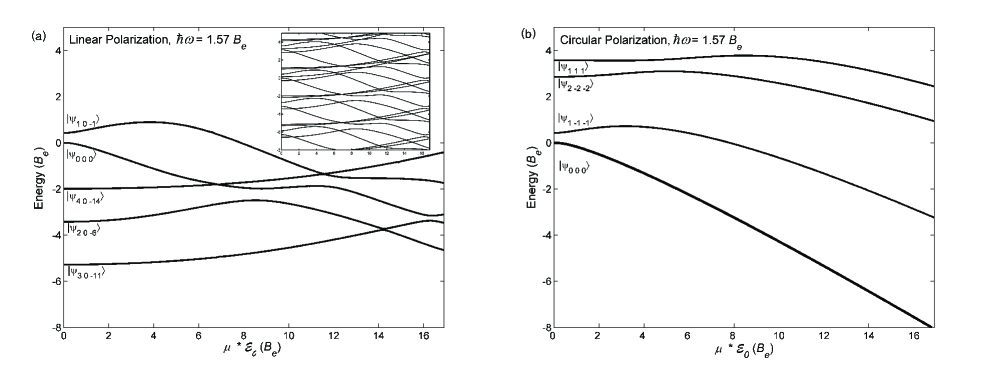
Figure 2: Energies of dressed states vs. applied microwave electric field strength. State labels are zero-field basis states $\left|{\psi_{Jmn}}\right\rangle$, as discussed in the main text. Only the subspace connected to $\left|{\psi_{000}}\right\rangle$ is shown. For this figure we have chosen a typical working value of the microwave frequency, $\hbar\omega=1.57B_{e}$. (a) Linear polarization $\mbox{\boldmath$\epsilon$}=\hat{z}$. In this calculation, $J_{max}=5$ and $n_{max}=20$. For clarity, only one dressed state for each initial value of $J<J_{max}$ is shown in the main diagram. (The inset shows the full Hilbert space included in the calculation; the pattern of levels is repeated for states with photon number $n^{\prime}=n\pm 2k$, where $k$ is any integer.) Note the large avoided crossings with the state that originates as $\left|{\psi_{000}}\right\rangle$ at zero field; the crossing of states labeled $\left|{\psi_{000}}\right\rangle$ and $\left|{\psi_{4\,0\,-14}}\right\rangle$ is also avoided, but the separation is too small to see in this diagram. (b) Circular polarization $\mbox{\boldmath$\epsilon$}=(\hat{x}-i\hat{y})/\sqrt{2}$. In this calculation, $J_{max}=10$ and $n_{max}=10$. All states of the coupled subspace in the plotted energy region are shown. Note the monotonic behavior and lack of avoided crossings for the $\left|{\psi_{000}}\right\rangle$ state.

The presence of these avoided crossings makes microwave traps using linearly polarized fields rather unattractive. Physically, as a molecule moves from regions of low to high field strength (either spatially or temporally), it is susceptible to absorption of multiple microwave photons, resulting in both a significant degree of rotational excitation, and a reduction in effective trap depth relative to our previous expectations. This situation corresponds to adiabatic following of the energy curve through an avoided crossing, leading to effective transfer from the initial state $\left|{\psi_{00n}}\right\rangle$ to a final state $\left|{\psi_{J^{\prime}0(n-k)}}\right\rangle$. From simple estimates of the time scales for change of $\mathcal{E}_{0}$ under likely physical conditions, we find that adiabatic following is probable even for crossings that are too small to observe in Fig. 2(a), so that a reliable prediction for the behavior of the system may be difficult without very detailed modeling of the molecular trajectories. We note in passing that this conclusion regarding linearly polarized fields may be too pessimistic for molecules with different structure, such as an inversion doublet with splitting much less than the rotational constant (where the microwave frequency should be detuned to the red of the doublet transition). However, we have not tried to analyze such a case explicitly.

Remarkably, the desired simple behavior of the microwave trap can be recovered by using a circularly polarized field, e.g. with $\mbox{\boldmath$\epsilon$}=(\hat{x}-i\hat{y})/\sqrt{2}$. In this case, absorption (emission) of k photons is necessarily accompanied by a change in angular momentum projection $\Delta m=-k(k)$. The critical difference from the case of linear polarization is that for the $\left|{J=0,m=0}\right\rangle$ state of interest, net absorption or emission of $k$ photons requires coupling to a state with angular momentum $J^{\prime}\geq m^{\prime}=k$, which is, for any field strength, separated in energy from the $\left|{J=0,m=0}\right\rangle$ state by $E(J^{\prime})-E(J=0)>2B_{e}k$. Thus, for a red detuned microwave trap (with $\hbar\omega<2B_{e}$), there are simply no resonant multiphoton transitions possible from the $\left|{J=0,m=0}\right\rangle$ state. This dramatically simplifies the behavior of ${\Delta E}$ as a function of $\mathcal{E}_{0}$, compared to the case of linear polarization. The manifold of coupled states that comprise the relevant Hilbert space for the case of circular polarization is shown in Fig. 1(b).

The molecular part of the off-diagonal matrix elements used for explicit calculations of the circular-polarization case are

$$\left\langle{J^{\prime},m^{\prime}}\right|\mathbf{n}\cdot\mbox{\boldmath$\epsilon$}^{*}\left|{J,m}\right\rangle=\left\langle{J,m}\right|\mathbf{n}\cdot\mbox{\boldmath$\epsilon$}\left|{J^{\prime},m^{\prime}}\right\rangle=$$

$$\frac{1}{\sqrt{2}}\left\langle{J^{\prime},m^{\prime}}\right|\sin{\theta}e^{i\varphi}\left|{J,m}\right\rangle=$$

$$\frac{1}{\sqrt{2}}\int{Y_{J^{\prime}}^{m^{\prime*}}\sin{\theta}e^{i\varphi}Y_{J}^{m}d\Omega}=$$

$$\left\{\frac{\sqrt{J-m-1}\sqrt{J-m}}{\sqrt{2J-1}\sqrt{2J+1}}\,\delta_{J^{\prime},J-1}+\right.$$

$$\left.\frac{\sqrt{J+m+1}\sqrt{J+m+2}}{\sqrt{2J+1}\sqrt{2J+3}}\,\delta_{J^{\prime},J+1}\right\}\delta_{m^{\prime},m+1}.$$ (6)

Typical results of the calculation are shown in Fig. 2(b). For moderately large fields such that $\mu\mathcal{E}_{0}\gtrsim B_{e}$, we find the desired (and originally expected) behavior ${\Delta E}\approx-\alpha\mathcal{E}_{0}$, where the proportionality factor $\alpha$ is roughly constant over a wide range of $\mathcal{E}_{0}$, is of order $\alpha\sim\mu/2$, and is maximal when the detuning $\Delta$ is minimized.

III Realistic design parameters for a microwave trap

The requirement for a circularly-polarized field, along with a desire to maintain an open geometry for optical and other access to the trap region, has led us to consider Fabry-Perot type resonators for the microwave trap. Such resonators are common in the mm-wave microwaveFPreview through optical regions Yariv , but rather less so in the microwave regime. Nevertheless, cavities with characteristics very similar to those required have been demonstrated GrachevFP ; gridinputcoupler ; we closely follow the treatment of Ref. GrachevFP in our discussion here. Our goal is to outline a basic, realistic design for such a resonator, and discuss the volume, depth, and other characteristics of the resulting trap potential.

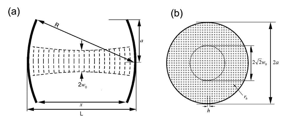
Figure 3: Layout of the microwave Fabry-Perot cavity. Labeled dimensions are defined in the main text. The figures are in scale with the nominal dimensions described in the text. (a) View from side. The dashed lines indicate the TEM₀₀ field mode. (b) View from input end. The grid of holes for partial transmission of the incident power is shown. The beam spot size at the mirror is $2w(z)=2\sqrt{2}w_{0}.$

We consider a symmetric, spherical-mirror Fabry-Perot cavity. We assume a confocal geometry, where the mirrors have spacing $L$ and radius of curvature $R=L$, and define the $z$-axis along the symmetry axis of the resonator, with $z=0$ midway between the mirrors. We consider the lowest-order transverse mode (TEM₀₀) in this cavity, for which the resonant condition is $L=(q+1/2)\lambda/2$, where $q$ is the integer number of half-wavelengths along the cavity axis; we choose $q$ odd to produce an antinode of the microwave electric field at $z=0$. For $q\gg 1$ so that the paraxial-ray approximation holds paraxialrayrefs , the electric field magnitude at time $t$ and position $(z,\rho,\phi)$ in cylindrical coordinates can be written as

$$\mbox{\boldmath$\mathcal{E}$}(z,\rho,\phi)=\mathcal{E}_{00}\frac{w_{0}}{w(z)}e^{-\rho^{2}/w^{2}(z)}\cdot$$

$$\cos{\left(kz-\textrm{tan}^{-1}(z/z_{0})+\frac{k\rho^{2}}{2\mathcal{R}(z)}\right)}\textrm{Re}\{\mbox{\boldmath$\epsilon$}e^{-i\omega t}\}.$$ (7)

Here we have introduced the wavevector $k=2\pi/\lambda$ and the standard Gaussian beam parameters: the minimum beam spot size $w_{0}$ and general spot size $w(z)=w_{0}\sqrt{1+z^{2}/z_{0}^{2}}$; the wavefront radius of curvature $\mathcal{R}(z)=z(1+z_{0}^{2}/z^{2})$; and the Rayleigh range $z_{0}=\pi w_{0}^{2}/\lambda$. For a confocal cavity, $w_{0}=\sqrt{\lambda L/(2\pi)}=\sqrt{Lc/\omega}$, and $z_{0}=L/2$. In the region of interest around the center of the resonator, the magnitude of the electric field is well-approximated by the expression

$$\mathcal{E}_{0}(z,\rho)=\mathcal{E}_{00}e^{-\rho^{2}/w_{0}^{2}}\cos{(2\pi z/\lambda)}\approx$$

$$\mathcal{E}_{00}(1-\frac{1}{2}\frac{8\pi}{(q+1/2)\lambda^{2}}\rho^{2}-\frac{1}{2}\frac{4\pi^{2}}{\lambda^{2}}z^{2}).$$ (8)

Thus, the trap formed by the field antinode around the origin is approximately harmonic in all directions, and has volume of $\sim\lambda^{3}$. Fig. 3 shows the geometric layout of the trap.

Suppose the input and output mirrors have amplitude transmission coefficients $t_{in}=t$ and $t_{out}=0$, respectively; loss coefficients $\gamma_{in}=\gamma_{out}=\gamma\ll 1$; and reflection coefficients $r_{in}=\sqrt{1-\gamma^{2}-t^{2}}$ and $r_{out}=r\sqrt{1-\gamma^{2}}$, respectively. For mirrors constructed of metal with resistivity $\rho$, it is easily shown that $\gamma=(8\epsilon_{0}\rho\omega)^{1/4}$ Jackson . The nonzero transmission $t$ of the input mirror can be engineered by perforating the mirror with an array of small holes of radius $r_{h}\ll\lambda/4\pi$, in a square grid with spacing $h<\lambda$. This yields a transmission coefficient $t=\frac{16\pi}{3}\frac{r_{h}^{3}}{h^{2}\lambda}$ GrachevFP . These conditions require that the thickness of the metal, $d$, satisfy $d\ll\delta\ll 2r_{h}$, where $\delta$ is the skin depth of the metal at frequency $\omega$: $\delta=\sqrt{2\rho/(\mu_{0}\omega)}$. We assume that the mirrors are of sufficiently large radius $a$ that diffractive losses $\gamma_{d}$ are negligible; this is satisfied when $\gamma_{d}=e^{-a^{2}/(2w_{0}^{2})}\ll\gamma$.

It is straightforward to show that, for a given microwave power incident on the input mirror of such a cavity, the electric field in the cavity is maximized when $t^{2}=2\gamma^{2}$; in this case the cavity has loaded $Q$-factor $Q_{l}=\pi(q+1/2)/(2\gamma^{2})$; the unloaded $Q$-factor, for the cavity without the input coupling grid, is $Q_{0}=2Q_{l}$. We assume microwave power $P_{in}$ is incident on the cavity input mirror, in the form of a mode-matched Gaussian beam with electric field distribution $\mathcal{E}_{in}(\rho,z=L/2)=\left({\mathcal{E}/\sqrt{2}}\right)e^{-\rho^{2}/(2w_{0}^{2})}$; here $P_{in}=\pi w_{0}^{2}\sqrt{\frac{\epsilon_{0}}{\mu_{0}}}\frac{\mathcal{E}_{i}^{2}}{4}$. In this case, the electric field at the center of the cavity is given by $\mathcal{E}_{0}=\sqrt{2}\mathcal{E}_{i}/\gamma$.

Next, in order to convey a sense of realistic parameters for the trap, we choose a specific set of nominal values for all the relevant parameters. We envision a microwave field at frequency $\omega=2\pi\times 15$ GHz, with wavelength $\lambda=2$ cm. (This is a convenient range for many oxide, fluoride, and nitride species.) For $q=$ 21 half-wavelengths in the cavity, $L=21.5$ cm and the beam waist size at the center (end) of the cavity is $w_{0}=$ 2.61 cm [$w(z=L/2)=$ 3.70 cm]. For room-temperature copper mirrors, using $\rho_{Cu}=1.7\times 10^{-8}\Omega\cdot$m, we find $\gamma=1.8\times 10^{-2}$ and $Q_{l}=1.0\times 10^{5}$. We take the mirror radius $a=0.4L=8.6$ cm; this gives $\gamma_{d}=4.4\times 10^{-3}\ll\gamma$. The required input coupling can be achieved with $h=0.5$ cm, $r_{h}=0.092$ cm. We believe that fabrication of a cavity with such parameters will be straightforward.

We assume a microwave input power $P_{in}=2$ kW. Such levels of power are commonly available from klystron-based satellite communication amplifiers, throughout much of the microwave band, i.e., in the frequency range of roughly 2-18 GHz. (Available power is a factor of 5-10 lower for higher frequencies up to $\sim 50$ GHz.) These amplifiers typically deliver the microwave power into standard waveguide; the required Gaussian mode for input to the cavity can be effectively obtained by launching into a corrugated scalar feed horn scalarfeedhorn or, less efficiency, with a standard pyramidal horn. Assuming perfect mode-matching at the input, we find a value for the peak electric field inside the cavity of $\mathcal{E}_{0}=\mathcal{E}_{00}=2.8$ MV/m. The parameter $\mu\mathcal{E}_{0}$, which governs the trap depth for a molecule with dipole moment $\mu$, is then $\mu\mathcal{E}_{0}=0.48$ cm${}^{-1}\mu$[D] = 0.69 K $\mu$[D]. Thus, for a typical range of parameters (such that $\mu\mathcal{E}_{0}\gtrsim B_{e}$ and thus ${\Delta E}\sim-\mu\mathcal{E}_{0}/2$), such a microwave trap can achieve trap depths ${\Delta E}\gtrsim 1$ K for molecular species with dipole moments $\mu\gtrsim 4$ D. We are currently constructing experiments optimized to trap the highly polar species SrO, with $\mu=8.9$ D and $B_{e}=0.34$ cm^-1 Herzberg . In this case we find explicitly a trap depth ${\Delta E}=-2.8$ K.

We have envisaged two possibilities for loading such a trap. In the simplest scheme, the trap is left off until a pulse of cold molecules enters the trapping region, at which time the microwave field is rapidly turned on. Note that the time scale to build up energy in the trap is $\tau=Q_{l}/\omega$; for our nominal parameters, $\tau=2\;\mu$s. This is much shorter than the typical time for a cold molecule to traverse the trapping region, so molecules can be effectively stopped when the trap potential suddenly appears. This ”trap door” loading scheme requires a source that delivers pulses of cold molecules already in their strong-field seeking ground state, such as the alternating gradient decelerator altgrad , or a source of weak-field seekers followed by a coherent pulse of resonant microwaves to transfer population to the ground state.

In the trap door scheme, it is not usually profitable to load more than a single pulse of molecules into the trap, since already-trapped molecules can escape while the trap is turned off for loading of subsequent pulses. However, it may be possible to load multiple pulses of weak-field seeking molecules into the microwave trap. Here, we envision optically pumping the molecules from the weak-field seeking excited state in which they are delivered, and into the trapped ground state optpumploading . The dissipation associated with optical pumping, combined with the rather different trap potentials for the strong- and weak-field seekers, makes the loading of one pulse completely transparent to any existing trapped molecules. Note that, in the absence of applied fields, parity selection rules forbid optical pumping from $J=1$ levels to the $J=0$ ground state. However, the presence of the microwave field breaks this selection rule, and makes it possible to perform the desired pumping. Such a scheme makes it attractive to load the trap using sources of weak-field seekers, such as the Stark decelerator originalStarkslower or the quadrupole filter + guide Rempefilterguide . For our experiments with SrO, we plan to use a version of the quadrupole guide, using a buffer-gas precooled source of laser-ablated SrO Doylecoldbeam .

IV Collisions in the microwave trap

As noted in the introduction, one of the main advantages of the microwave trap is that it holds molecules in their absolute ground state, so that two-body inelastic collisions are impossible. Here we point out that, in addition, molecules held in a microwave trap may be subject to very high rates of elastic collisions. This is attractive, since the re-thermalization associated with elastic collisions is a key step in the process of evaporative and/or sympathetic cooling.

The primary point of the discussion is that, in the center of the microwave trap, the molecules are subject to the large microwave electric field, which results in their nearly-complete electrical polarization. The r.m.s. expectation value of the dipole moment of the molecular state in the presence of the microwave field, $\left\langle{\mu}\right\rangle$, can be obtained simply from the earlier calculations; it is given simply by the slope of the ground-state energy vs. electric field curve, $\left\langle{\mu}\right\rangle=\partial({\Delta E})/\partial\mathcal{E}_{rms}=\sqrt{2}\partial({\Delta E})/\partial\mathcal{E}_{0}$. Under typical conditions, throughout most of the volume of the trap, $\left\langle{\mu}\right\rangle\sim\mu/2$. The bare dipole-dipole interactions between the polarized molecules are both very strong and of long range; this in turn greatly enhances the elastic collision cross-sections, compared to the case between unpolarized molecules.

Kajita Kajitasemiclassical ; Kajitacolder , and Bohn Bohnpolarcollisions ; BohnOHcollisions , have considered elastic collisions between electrically polarized molecules in a variety of different regimes, using rather different techniques. We are particularly interested here in collisions between strongly-polarized molecules at rather high temperatures ($T\gg 1$ mK, corresponding to the initial conditions in the trap). In this regime, Kajita has argued that a semi-classical calculation is valid Kajitasemiclassical . Although the discussion of Ref. Kajitasemiclassical explicitly focuses on collisions between weak-field seeking states in a static electric trap, it is straightforward to recast the elastic cross-section derived there in terms of the parameters used in this paper. Specifically, using from Ref. Kajitasemiclassical Eqs.(7), (8), and (10), Table 1, and the discussion following Eq.(10), we find the dipole-dipole elastic collision cross-section $\sigma$ between molecules of relative velocity $v$ and mass $m$ can be written as

$$\sigma \approx \frac{40\pi\sqrt{2}}{3}\frac{1}{4\pi\epsilon_{0}}\frac{\left\langle{\mu}\right\rangle^{2}}{\hbar v}$$ (9)

$$\approx \sqrt{\frac{m\textrm{[amu]}}{T\textrm{[K]}}}\left\langle{\mu\textrm{[D]}}\right\rangle^{2}\cdot 4\times 10^{-12}\textrm{cm}^{2}.$$

For the specific case of SrO, where $\left\langle{\mu}\right\rangle\approx 6.9$ D, $m=104$ amu, and (when initially trapped) $T={\Delta E}=2.8$ K, this yields a remarkably large cross-section $\sigma\approx 1.2\times 10^{-9}$ cm². This is an extraordinarily large cross-section, which will lead to a substantial elastic collision rate even with a relatively small number of initially-loaded molecules. We stress again the notable fact that $\sigma\propto T^{-1/2}$; this means that, as the sample cools, collision rates can be preserved with little difficulty.

The regime in which the result of Eq.(9) is valid appears to be rather broad. In particular, the semiclassical treatment (which assumes contributions from many partial waves) should break down significantly only when $\sigma\lesssim\sigma_{q}$, where $\sigma_{q}=4\pi(\hbar/mv)^{2}$ is the maximum quantum cross-section for a single partial wave. Using the numerical relation of Eq.(9), we find that the condition $\sigma/\sigma_{q}>1$ for the presumed validity of the semiclassical calculation implies a very weak condition on the temperature: $T>(m\textrm{[amu]})^{-3}\left\langle{\mu\textrm{[D]}}\right\rangle^{-4}\cdot 64\;\mu$K. Returning again to the example of SrO, $\sigma/\sigma_{q}>1$ for $T\gtrsim 3\times 10^{-14}$ K! It appears that the semiclassical relation of Eq.(9) is likely to remain valid under most realistic experimental conditions. It is notable that the scaling with $T$ appears to be borne out in the explicit calculations of Ref. BohnOHcollisions , for temperatures down to $T\sim 1\;\mu$K.

We point out, parenthetically, that the result of Eq.(9) can be approximately derived using an extremely simple model. We anticipate that in the semiclassical limit, the anisotropy of the dipole-dipole interaction will play a minor role in the average scattering properties. This leads us to consider the cross-section for scattering by an isotropic potential of the form $V_{iso}(r)=-\left\langle{\mu}\right\rangle^{2}/(4\pi\epsilon_{0}r^{3})$. It was shown by Julienne and Mies that for such a potential, a semiclassical description of scattering should be valid for sample temperatures

$$T>T_{Q}=\frac{2^{18}}{3^{12}}\frac{\hbar^{6}(4\pi\epsilon_{0})^{2}}{m^{3}\left\langle{\mu}\right\rangle^{4}};$$ (10)

for SrO under our conditions, $T_{Q}\approx 2\times 10^{-13}$ K, in reasonable agreement with the estimate above for the regime in which the semiclassical description is valid. In the extreme high-temperature limit ($T\gg T_{Q}$), the classical path of the scattered particle should be close to a straight line; this makes it possible to use the Eikonal approximation Sakurai , where (by invoking the optical theorem), the total elastic scattering cross-section can be written as

$$\sigma_{Eik}=-4\pi\int\limits_{0}^{\infty}{b(\cos{(2\Delta(b))}-1)db},$$ (11)

with

$$\Delta(b)=-\frac{1}{2v}\int\limits_{-\infty}^{\infty}{V_{iso}\left({\sqrt{b^{2}+z^{2}}}\right)dz}.$$ (12)

This yields the simple analytic solution

$$\sigma_{Eik}=2\pi^{2}\left\langle{\mu}\right\rangle^{2}/(4\pi\epsilon_{0}\hbar v).$$ (13)

The Eikonal solution for the anisotropic potential exhibits the same scaling as the proper semiclassical solution, and is numerically smaller by a factor of only $\sim 3$. It is not clear whether this difference arises principally because we have neglected the anisotropy of the interaction (particularly the repulsive part of the potential), or because the classical path deviates significantly from a straight line. Nevertheless, we find this derivation useful, for the straightforward way it leads to the correct scaling (and nearly correct magnitude) of the cross-section.

Finally, we point out the suitability of the microwave trap for performing sympathetic cooling of the trapped molecules, by contact with much colder laser-cooled atoms. The geometry of our proposed trap is very convenient for this purpose. The open distance between the edges of the mirrors (see Fig. 3) is $x=2L\left({\sqrt{1-(a/L)^{2}}-1/2}\right)=17.9$ cm , which is greater than the mirror diameter ($2a=17.2$ cm). Thus, there is sufficient open area to overlap 3 orthogonal laser beams in the center of the microwave trap, as required for a superposed atomic magneto-optic trap (MOT). In addition, the microwave field itself will form a weak, conservative trap for the atoms, analogous to that formed by a far off-resonant optical dipole trap. The microwave polarizability of atoms is virtually identical to the DC polarizability; the Stark shift of the atomic ground state in the presence of a DC electric field $\mathcal{E}_{DC}$ is typically written in the form ${\Delta E}_{atom}=-\alpha_{0}\mathcal{E}_{DC}^{2}/2$; for atomic Cs, $\alpha_{0}=6.61\times 10^{-39}$ C $\cdot$ m²/V Cspol . With our nominal trap parameters, and taking into account that the atoms respond to the r.m.s. AC electric field, $\mathcal{E}_{rms}=\mathcal{E}_{0}/\sqrt{2}$, we find a microwave trap depth for Cs of ${\Delta E}_{Cs}=-1.0$ mK, which is easily sufficient to hold all atoms collected in a standard MOT. Polarizabilities for all alkalis are similar. Atoms can be loaded into the microwave trap by rapidly turning on the microwave field after the MOT is loaded; since the volume of the microwave trap is much larger than a typical MOT dimension, transfer should be very efficient.

In this context, it is interesting to consider the elastic cross-section between an alkali atom such as Cs, and a molecule in the trap. This cross-section receives a contribution from the fact that the alkali atoms are also slightly polarized in the microwave field, with an rms expectation value of the atomic dipole moment of $\left\langle{\mu}\right\rangle_{atom}=\alpha_{0}\mathcal{E}_{0}/\sqrt{2}$. Taking into account only the dipole-dipole interaction between atom and molecule, it is possible to calculate the cross-section by a simple modification of Eq.(9) to take into account scattering by unequal dipoles. This should represent at least a lower bound on the atom-molecule elastic cross-section, which could in principle be significantly enhanced by shorter-range effects (such as the direct interaction of the dipolar field of the molecule with the polarizability of the atom) that are not considered here. For Cs under our nominal conditions, we find $\left\langle{\mu}\right\rangle_{Cs}=\alpha_{0}\mathcal{E}_{0}/\sqrt{2}=3\times 10^{-3}$ D and a Cs-SrO cross section, due to dipole-dipole interactions, of $\sigma_{Cs-SrO}\approx 10^{-12}$ cm² at $T\sim 1$ K. This is large enough to enable rapid sympathetic cooling with typical atomic densities achieved in a MOT (see e.g. Ref. ourRbCspapers ).

V Conclusions

We have argued that microwave-based traps for polar molecules have many attractive properties. In particular, using this technology it appears possible to create large, deep traps for absolute ground state molecules. Collisions between molecules in these traps should have very large elastic cross-sections and no two-body inelastic losses, opening the realistic possibility for evaporative cooling of molecules. Our discussion has stressed the design of such a trap for diatomic molecules in rigid rotor states, using an open trap geometry. With minor modifications from our nominal design parameters, this trap would be well-suited to a wide variety of species; in particular, it works well for molecules with rotational constants $B_{e}$ in the range of roughly 0.05 -0.5 cm^-1 and intrinsic dipole moments $\mu$ of at least few Debye. This covers many diatomics with the lightest constituent atom in the first two complete rows of the periodic table (Li - Cl). Additional design considerations would be required to optimize the microwave trap for hydrides, or for molecules with inversion or lambda-doublet structures; however, we think it is likely that a similar type of technology could prove useful in these cases as well.

There also remain a number of interesting questions concerning the operation of such traps. In particular, possible inelastic losses due to three-body processes, particularly those resulting in chemical reactions, will be interesting to study in this strongly-interacting system. In addition, the dynamics of evaporative cooling in such traps may be very different from the well-studied cases in atomic physics, as the elastic cross-sections become so large that the dipolar gas has a non-negligible viscosity. We look forward to future studies of such issues. As mentioned above, we have experiments underway to load the strongly polar species SrO into such a trap, where we anticipate many interesting developments.

We gratefully acknowledge support from NSF grant DMR-0325580, the David and Lucile Packard Foundation, and the W.M. Keck Foundation.

References

- (1) P.S. Julienne, Nature 424, 24 (2003); B.G. Levi, Phys. Today 53, 46 (2000).
- (2) D.DeMille, Phys. Rev. Lett. 88, 067901 (2002).
- (3) M.A. Baranov, M.S. Mar’enko, Val.S. Rychkov, and G.V. Shlyapnikov, Phys. Rev. A 66, 013606 (2002).
- (4) K. Góral, L. Santos, and M. Lewenstein, Phys. Rev. Lett. 88, 170406 (2002), and references therein.
- (5) M. Olshanii, Phys. Rev. Lett. 81, 938-941 (1998); D. S. Petrov and G. V. Shlyapnikov, Phys. Rev. A 64, 012706 (2001); U. Al Khawaja, J.O. Andersen, N.P. Proukakis, and H.T.C. Stoof, Phys. Rev. A 66, 013615 (2002); D.S. Petrov, M.A. Baranov, and G.V. Shlyapnikov, Phys. Rev. A 67, 031601 (2003).
- (6) E. Bodo, F. Gianturco, and A. Dalgarno, J. Chem. Phys. 116, 9222 (2002), and references therein.
- (7) A.V. Avdeenkov and J. L. Bohn, Phys. Rev. Lett. 90, 043006 (2003).
- (8) M. Kozlov and L. Labzowsky, J. Phys. B 28, 1933 (1995).
- (9) A.J. Kerman, J.M. Sage, S. Sainis, T. Bergeman, and D. DeMille, Phys. Rev. Lett. 92, 033004 (2004); A.J. Kerman, J. M. Sage, S. Sainis, T. Bergeman, and D. DeMille, Phys. Rev. Lett. 92, 153001 (2004).
- (10) M.W. Mancini et al., Phys. Rev. Lett. 92, 133203 (2004).
- (11) E. Eyler and W. Stwalley, private communication.
- (12) G. Modugno, G. Roati, and M. Inguscio, Fortschr. Phys. 51, 396 (2003); A. Simoni et al., Phys. Rev. Lett. 90, 163202 (2003).
- (13) J.D. Weinstein et al., Nature 395, 148 (1998).
- (14) H.L. Bethlem et al., Nature 406, 491 (2000).
- (15) S.A. Rangwala et al., Phys. Rev. A 67, 043406 (2003).
- (16) M.S. Elioff, J.J. Vaentini, and D.W. Chandler, Science 302, 1940 (2003).
- (17) J.R. Bochinski et al., Phys. Rev. Lett. 91, 243001 (2003).
- (18) J. L. Bohn, Phys. Rev. A 63, 052714 (2001).
- (19) M. Kajita, Eur. Phys. J. D 20, 55 (2002).
- (20) M. Kajita, Eur. Phys. J. D 23, 337 (2003).
- (21) A. Volpi and J.L. Bohn, Phys. Rev. A 65, 052712 (2002).
- (22) M. Kajita, Phys. Rev. A 69, 012709 (2004) argues that evaporative cooling can be effective for fermionic molecules in electrostatic traps, at very low temperatures.
- (23) H. J. Loesch and B. Scheel, Phys. Rev. Lett. 85, 2709 (2000).
- (24) F.M.H. Crompvoets, H.L. Bethlem, R.T. Jongma, and G. Meijer, Nature 411, 174 (2001).
- (25) T. Junglen, et al., Phys. Rev. Lett. 92, 223001 (2004).
- (26) See e.g. C.H. Townes and A.L. Shawlow, Microwave Spectroscopy (McGraw-Hill, New York, 1955).
- (27) S. Chu, J.E. Bjorkholm, A. Ashkin, and A. Cable, Phys. Rev. Lett. 57, 314 (1986); J.D. Miller, R.A. Cline, and D.J. Heinzen, Phys. Rev. A 47, R4567 (1993).
- (28) C. Cohen-Tannoudji, J. Dupont-Roc, and G. Grynberg, Atom-Photon Interactions: Basic Processes and Applications (John Wiley & Sons, New York, 1992).
- (29) See e.g. R.N. Clarke and C.B. Rosenberg, J. Phys. E 15, 9 (1982).
- (30) See e.g. A. Yariv, Quantum Electronics (Third Edition) (John Wiley & Sons, New York, 1989).
- (31) L.P. Grachev, I.I. Esakov, S.G. Malyk, and K.V. Khodataev, Tech. Phys. 46, 709 (2001).
- (32) T. Matsui, IEEE Trans. Microw. Theory Tech. 41, 1710 (1993).
- (33) J. Tuovinen, IEEE Trans. Antennas Propag. 40, 391 (1992); S. Nemoto, Appl. Opt. 29, 1940 (1990); T. Takenaka, M. Yokota, and O. Fukumitsu, J. Opt. Soc. Am. A 2, 826 (1985); G.P. Agrawal and M. Lax, Phys. Rev. A 27, 1693 (1983).
- (34) J. D. Jackson, Classical Electrodynamics (Second Edition) (John Wiley & Sons, New York, 1975), Problem 7.4.
- (35) R. E. Lawrie and L. Peters Jr; IEEE Trans. Antennas Propag. 14, 605 (1966).
- (36) K.P. Huber and G. Herzberg, Molecular Spectra and Molecular Structure IV., Constants of Diatomic Molecules (Von Nostrand Reinhold, New York, 1979).
- (37) H.L. Bethlem, A.J. A. van Roij, R.T. Jongma, and G. Meijer, Phys. Rev. Lett. 88, 133003 (2002); M.R. Tarbutt et al., Phys. Rev. Lett. 92, 173002 (2004).
- (38) A similar trap loading scheme is discussed in: S.Y.T. van de Meerakker, R.T. Jongma, H.L. Bethlem, and G. Meijer, Phys. Rev. A 64, 041401R (2001); S.Y.T. van de Meerakker et al., Phys. Rev. A 68, 032508 (2003).
- (39) H.L. Bethlem, G. Berden, and G. Meijer, Phys. Rev. Lett. 83, 1558 (1999).
- (40) N. Brahms et al., Bull. Am. Phys. Soc. 49, 52 (2004); J. Doyle et al., to be published.
- (41) A.V. Avdeenkov and J.L. Bohn, Phys. Rev. A 66, 052718 (2002).
- (42) P.S. Julienne and F.H. Mies, J. Opt. Soc. Am. B 6, 2257 (1989).
- (43) See e.g. J. J. Sakurai, Modern Quantum Mechanics (Revised Edition) (Addison-Wesley, Reading, MA, 1994).
- (44) J. M. Amini and H. Gould, Phys. Rev. Lett. 91, 153001 (2003).