Narrow Line Cooling and Momentum-Space Crystals
Abstract
Narrow line laser cooling is advancing the frontier for experiments ranging from studies of fundamental atomic physics to high precision optical frequency standards. In this paper, we present an extensive description of the systems and techniques necessary to realize 689 nm - narrow line cooling of atomic 88Sr. Narrow line cooling and trapping dynamics are also studied in detail. By controlling the relative size of the power broadened transition linewidth and the single-photon recoil frequency shift, we show that it is possible to continuously bridge the gap between semiclassical and quantum mechanical cooling. Novel semiclassical cooling process, some of which are intimately linked to gravity, are also explored. Moreover, for laser frequencies tuned above the atomic resonance, we demonstrate momentum-space crystals containing up to 26 well defined lattice points. Gravitationally assisted cooling is also achieved with blue-detuned light. Theoretically, we find the blue detuned dynamics are universal to Doppler limited systems. This paper offers the most comprehensive study of narrow line laser cooling to date.
I Introduction
Narrow line magneto-optical traps (MOTs) are rapidly becoming powerful tools in a diverse array of experimental studies. These unique and versatile systems have, for example, already been used as integral components in obtaining fully maximized MOT phase-space densities Katori3 , nuclear-spin based sub-Doppler cooling Maru ; JILA1d , all-optical quantum degenerate gases Takasu03 , and recoil-free spectroscopy of both dipole allowed Katori4 and doubly-forbidden Katori5 optical transitions. In the future, narrow line MOTs promise to revolutionize the next generation of high precision optical frequency standards Katori6 ; Curtis ; PTB . Narrow line cooling, via the relative size of the transition natural width and the single-photon recoil frequency shift , also displays a unique set of thermal-mechanical laser cooling dynamics. In a previous paper Loftus3 , we explored these behaviors by cooling 88Sr on the - intercombination transition. In the present work, we significantly expand upon this discussion and provide a comprehensive description of the experimental techniques used to realize and study - cooling and trapping.
Fully understanding narrow line laser cooling requires first clarifying the difference between broad and narrow Doppler cooling lines. Broad lines, historically used for nearly every laser cooling experiment Metcalf , are defined by / 1. The 461 nm 88Sr - transition shown in Fig. 1(a), which typifies a broad line, has, for example, / 3103. In this case, , or more generally the power-broadened linewidth , is the natural energy scale. Here, = is defined by the saturation parameter = / where () is the single-beam peak intensity (transition saturation intensity). Semiclassical physics thus governs the cooling process and the photon recoil, although essential to quantitatively understanding energy dissipation Wineland , serves more as a useful conceptual tool than a dominant player in system dynamics. Moreover, gravity is essentially negligible since the ratio of the maximum radiative force to the gravitational force, = /2, is typically on the order of 105, where , , , and are Plank’s constant, the light field wavevector, the atomic mass, and the gravitational acceleration, respectively.
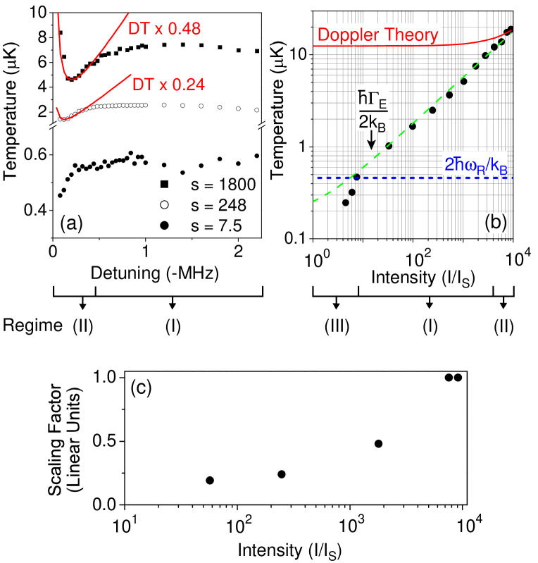
In contrast, narrow Doppler cooling lines are characterized by / 1. The 689 nm 88Sr - transition used in this work, for example, has / = 1.6 where /2 (/2 = /4) is 7.5 kHz (4.7 kHz). In this case, the relevant thermal-mechanical energy scale and thus the underlying semiclassical or quantum mechanical nature of the cooling depends on . Details of a given cooling process are then set by the laser detuning 2 = = where () is the laser (atomic resonance) frequency. In particular, 0 - MOT dynamics can be divided into three qualitatively distinct regimes, hereafter labeled (I - III), defined by the relative size of , , and . In regime (III), corresponding to trapping beam intensities on the order of = 3W/cm2 or 1, is the natural energy scale. Here, single photon recoils and consequently, quantum physics, govern trap dynamics. This situation enables limiting temperatures of roughly half the photon recoil limit ( = 2/ = 460 nK, where is Boltzmann’s constant) despite the incoherent excitation provided by the trapping beams Metcalf ; dalibard89 .
Conversely, for 1 the system evolves toward semiclassical physics where and hence is the dominant energy scale. In this case, cooling and motional dynamics are determined by the relative size of and . In regime (II), the radiative force produces damped harmonic motion and, in analogy to standard Doppler cooling, MOT thermodynamics set entirely by the velocity dependence of the force Lett ; JILA1c . For these conditions, the expected - and -dependent temperature minima are observed, although with values globally smaller than standard Doppler theory predictions. Alternatively, in regime (I) where , the atom-light interaction is dominated by single-beam photon scattering and trap thermodynamics become intimately linked to both the velocity and the spatial dependence of the force. Here, gravity plays an essential role as the ratio for the - transition is only 16. Consequently, the atoms sag to vertical positions where the Zeeman shift balances , leading to -independent equilibrium temperatures.
Narrow line cooling also displays a unique set of 0 thermal and mechanical dynamics. For these experiments, the atomic gas is first cooled to K temperatures and then is suddenly switched from 0 to 0. Subsequently, the sample evolves from a thermal distribution to a discrete set of momentum-space packets whose alignment matches lattice points on a three-dimensional (3D) face-centered-cubic crystal Com1 . Up to 26 independent packets are created with - and -dependent lattice point filling factors. Note this surprising behavior occurs in the setting of incoherent excitation of a non-degenerate thermal cloud. To obtain qualitative insight into the basic physics, we begin with an analytic solution to the one-dimensional (1D) semiclassical radiative force equation. Here, we show that 0 excitation enables ”positive feedback” acceleration that efficiently bunches the atoms into discrete sets of - and -dependent velocity space groups. A simple generalization of the 1D model is then used to motivate the experimentally observed 3D lattice structure. This intuitive picture is then confirmed with numerical calculations of the final atomic velocity and spatial distributions. Using the numerical calculations, we also show that 0 momentum-space crystals are a universal feature of standard Doppler cooling and that observations should be possible, although increasingly impractical, with broad line molasses.
Finally, we demonstrate that directly influences 0 thermodynamics, enabling cooling around a - and -dependent velocity where gravity balances the radiative force. Observed values for agree well with numerical predictions while cooling is evident in distinctly asymmetric cloud spatial distributions that appear in both numerical calculations of the cooling process and the experiment. As with momentum crystal formation, gravitationally assisted 0 cooling is universal to Doppler limited systems. In the more typical case where 105, however, equilibrium temperatures () are on the order of hundreds of milli-Kelvin (100 m/s) rather than the more useful micro-Kelvin ( 10 cm/s) values achieved with narrow lines.
The remainder of this paper is organized as follows. Section II gives an overview of the 461 nm - MOT used to pre-cool 88Sr to 2.5 mK. metastable excited-state magnetic traps that are continuously loaded by the - cooling cycle are also described. Section III details the highly stabilized 689 nm light source and the process used to transfer 88Sr from the - MOT to the - MOT. Descriptions of the techniques used to control and study - laser cooling are also provided. Sections IV and V then focus on 0 mechanical and thermal dynamics, respectively. Finally, section VI explores 0 cooling and momentum-space crystals. Conclusions are given in section VII.
II - MOT Pre-Cooling
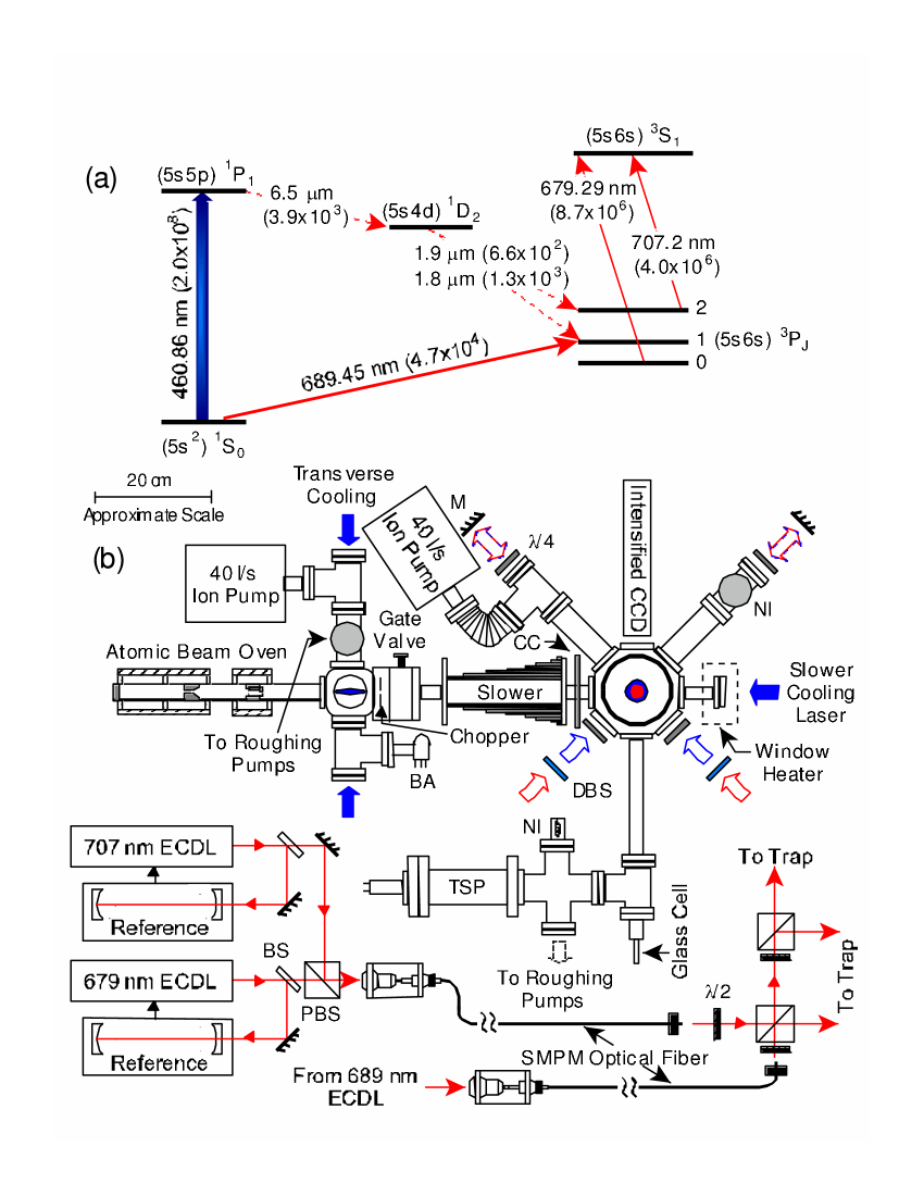
Pre-cooling 88Sr to milli-Kelvin temperatures is an essential requirement for observing - cooling and trapping dynamics Katori3 . For this purpose, as shown by Fig. 1(b), we use a standard six-beam 461 nm - MOT that is loaded by a Zeeman slowed and transversely cooled atomic beam. The atomic beam is generated by an effusion oven (2 mm nozzle diameter) whose output is angularly filtered by a 3.6 mm diameter aperture located 19.4 cm from the oven nozzle. Separate heaters maintain the oven body (nozzle) at 525 oC (725 oC), resulting in a measured flux (divergence half-angle) of 31011 atoms/s (19 mrad). The atomic beam is then transversely cooled by 2-dimensional 461 nm optical molasses. The elliptical cross-section molasses laser beams have a 1/e2 diameter of 3 cm ( 4 mm) along (normal to) the atomic beam propagation axis, contain 10 - 20 mW of power, and are detuned from the - resonance by -15 MHz. Stray magnetic fields in the transverse cooling region are less than 1 G. Subsequently, the atomic beam passes through a 6.4 mm diameter electro-mechanical shutter and a gate valve that allows the oven to be isolated from the rest of the vacuum system.
After exiting the transverse cooling region, the atomic beam enters a water cooled 20 cm long constant deceleration Zeeman slower slower with a peak magnetic field of 600 G, corresponding to a capture velocity of 500 m/s. The 461 nm Zeeman slower cooling laser is detuned from the - resonance by -1030 MHz, contains 60 mW of power, and is focused to approximately match the atomic beam divergence. The window opposite the atomic beam is a z-cut Sapphire optical flat that is vacuum sealed via the Kasevich technique Kasevich , broadband anti-reflection coated on the side opposite the chamber, and heated to 200 oC to prevent the formation of Sr coatings. The alternating current window heater, which produces a small stray magnetic field, is only operated during the - MOT pre-cooling phase. A separate compensation coil reduces the slower magnetic field magnitude (gradient) to 100 mG ( 8 mG/cm) at the trapping region, located 15 cm from the slower exit. Stray magnetic fields at the trap are further nulled by three sets of orthogonally oriented Helmholtz pairs.
The trapping chamber is a cylindrical octagon with six 2 3/4” (two 6”) ports in the horizontal x-y plane (along gravity z-axis). All windows are broadband anti-reflection coated. The MOT anti-Helmholtz coils, oriented such that the axial magnetic field gradient dBz lies along gravity, are mounted on a computer controlled precision linear track that allows the coil center to be translated from the trapping chamber to a 1 cm 1 cm 4 cm rectangular glass cell. The coils are constructed to provide window-limited optical access to the geometric center of the trapping chamber and produce axial gradients of 0.819 G/(cm-A). The gradient is linear over a spatial range of 3 cm in both the axial and transverse directions. Current in the coils is regulated by a computer controlled servo and monitored with a Hall probe. For the - MOT, the axial magnetic field gradient dBz/dz = dBz = 50 G/cm.
The trapping chamber is evacuated by a 40 /s Ion pump and a Titanium sublimation pump while the oven chamber uses a 40 /s Ion pump. The two chambers are separated by a 6.4 mm 45 mm cylindrical differential pumping tube located between the electro-mechanical shutter and the gate valve. Typical vacuum levels in the oven, trapping, and glass cell chambers during operation of the atomic beam are 210-8 Torr, 1.510-9 Torr, and 310-10 Torr, respectively.
461 nm cooling and trapping light is produced by frequency doubling the output from a Ti:Sapphire laser in two external buildup cavities doubler that together produce 220 mW of single-mode light. The 461 nm light is then offset locked to the - resonance by saturated absorption feedback to the Ti:Sapphire laser. Relative frequencies of the transverse cooling, Zeeman slower, and trapping laser beams are controlled with acousto-optic modulators (AOMs) which are also used as shutters. Additional extinction of 461 nm light is provided by electro-mechanical shutters. The intensity stabilized trapping beams have 1/e2 diameters of 3 cm, are detuned from the - resonance by -40 MHz, and typically have a total power of 30 mW. For these settings, we find the - MOT population is maximized. Further increases in, for example, the trapping beam power simply increases the cloud temperature. - MOTs are monitored with a charge-coupled-device (CCD) camera and a calibrated photodiode. Typical trap lifetimes, populations, and temperatures are 20 ms, 3107, and 2.5 mK, respectively.
As shown by Fig. 1(a), operation of the - MOT efficiently populates the ground-state-like metastable excited-state ( 500 s radiative lifetime Katori1 ) via radiative decay. Consequently, - MOT lifetimes are typically limited to 10 - 50 ms Loftus4 ; JILA1a ; JILA1b . To overcome this loss process, population is re-pumped to the ground-state via the channel by driving the 707 nm - and 679 nm - transitions with two external cavity diode lasers (ECDLs). Each laser is locked to a reference cavity that is simultaneously locked to a frequency stabilized helium neon laser. Double-passed AOMs are then used to tune the absolute laser frequencies. After passing through a single-mode polarization-maintaining optical fiber, the co-propagating 707 nm and 679 nm laser beams are expanded to a 1/e2 diameter of 1 cm and delivered to the - MOT. An AOM located before the beam expansion optics allows for rapidly turning the beams either on or off ( 1 s transition time). At the trap, the 707 nm (679 nm) beam contains 1.5 mW (2.5 mW) of power, resulting in an optical re-pumping time of 100 s. With both lasers operating, the - MOT population and lifetime are typically enhanced by 10 and 15, respectively, with the former value limited by atomic beam induced trap loss.
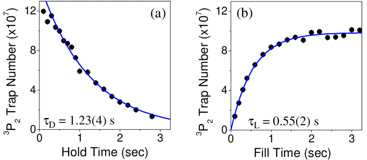
Along with contributing to - MOT loss, radiative decay continuously loads milli-Kelvin atoms in the (m=1,2) states into a magnetic trap formed by the - MOT quadrupole magnetic field Loftus1 ; Katori2 ; Loftus2 ; JILA1b ; Killian ; Hemmerich . Importantly, these samples are expected to display a wealth of binary collision resonances that arise due to an interplay between anisotropic quadrupole interactions and the local magnetic field Derevianko ; GreenePRL ; GreenePRA . Qualitatively similar processes and hence, collision resonances, are predicted for polar molecules immersed in electrostatic fields Bohn . Studies of metastable Sr collision dynamics will thus likely impact the understanding of a diverse range of physical systems. To pursue these studies, we plan to first load state atoms into the quadrupole magnetic trap and then mechanically translate Lewandowski the sample to the glass cell chamber. Subsequently, a tight Ioffe-Pritchard magnetic trap will be used to perform a variety of collision experiments.
As a first step in this direction we have loaded 108 (m=1,2) state atoms into the quadrupole magnetic trap and achieved trap lifetimes 1 s. For these measurements, the trap is first loaded by operating the - MOT for a variable fill time. The 461 nm cooling and trapping lasers and the atomic beam are then switched off. Following a variable hold time, the 461 nm trapping beams and the 707 nm and 679 nm re-pumping beams are switched on, enabling the magnetic trap population NM to be determined from 461 nm fluorescence Katori2 . Figure 2(a) shows NM versus hold time for a fill time of 2 s while Fig. 2(b) gives NM versus fill time at a fixed hold time of 400 ms. For both, dBz = 50 G/cm, giving a magnetic trap depth of 30 mK. The - MOT lifetime (steady-state population) is 16 ms (2.8107). The observed 1.23(4) s exponential decay time agrees well with the expected 1.3 s vacuum limited value extracted from measurements reported in Ref. Killian at higher pressures. In contrast, the significantly shorter 0.55(2) s fill time implies that additional loss processes are operative during the loading phase, possibly due to interactions between atoms in the or states with - MOT atoms or the atomic beam Stuhler . This idea is supported by the magnetic trap loading rate. For the parameters used here, the observed rate of 2.7(5)108 atoms/s is 2 smaller than the theoretically predicted value of 5.4(1.8)108 atoms/s Loftus1 where the theory only accounts for relevant branching ratios in the (m=1,2) radiative cascade. Similar discrepancies between observed and predicted loading rates were reported in Ref. Killian .
III - MOT Loading and Detection
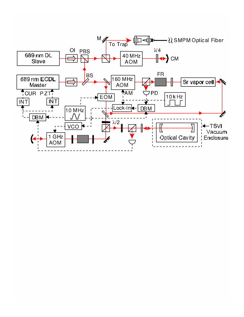
Exploring 689 nm - narrow line cooling dynamics requires a laser system whose short-term linewidth is small compared to the 7.5 kHz transition natural width. In addition, the absolute laser frequency must be referenced, with similar stability, to the - transition and be tunable over a range of 10 MHz. Figure 3 shows the 689 nm laser stabilization and control system consisting of a master-slave ECDL, a temperature stabilized and vibration isolated passive optical reference cavity, and a Sr saturated absorption spectrometer.
The linewidth of the master ECDL is first narrowed by locking the laser to a stable optical reference cavity via the Pound-Drever-Hall technique PDH . The cavity consists of high reflectivity Zerodour substrate mirrors that are optically contacted to a Zerodour spacer. The measured cavity finesse (free spectral range) at 689 nm is 3800 (488.9 MHz), giving a linewidth for the TEM00 mode of 130 kHz. To isolate the cavity from environmental perturbations, the cavity is suspended by two thin wires inside a temperature stabilized can that is evacuated to 10-6 Torr and mounted on vibration damping material. The absolute cavity frequency is tuned by double-passing the 689 nm light sent to the cavity through a 1 GHz AOM. The electronic feedback, with an overall bandwidth of 2 MHz is divided into a slow loop that adjusts the piezo-electric mounted ECDL grating and a fast loop that couples to the diode laser current. With the cavity lock engaged, in-loop analysis shows that jitter in the cavity-laser lock is 1 Hz.
To further evaluate the performance of the 689 nm laser system, the short-term laser linewidth is determined by beating the cavity-locked 689 nm light against a femto-second comb that is locked to a second optical cavity Jones . Here, we find a short-term linewidth of 300 Hz, where the measurement is limited by the optical fiber connecting the 689 nm light to the femto-second comb. Next, the absolute stability of the 689 nm laser is evaluated by beating the cavity locked 689 nm light against a femto-second comb that is locked to a Hydrogen maser via a fiber optical link to NIST maser . From these measurements, the laser-cavity system drifts 400 mHz/s and has a 1 s stability of 410-13 (i.e., 180 Hz) with the former value limited by cavity drift and the latter value limited by the effective maser noise floor. To eliminate the slow 689 nm cavity induced drift, the master ECDL is next locked to the - resonance via saturated absorption feedback to the 1 GHz AOM. For added stability, a DC magnetic field is applied to the Sr vapor cell and the spectrometer is set to perform frequency modulation spectroscopy on the - (m=0) transition. With the system fully locked, the 1 s stability (drift rate) is then 410-13 ( 80 mHz/s).
A portion of the 689 nm master ECDL output is next used to injection lock a 689 nm slave diode laser. The slave laser output, after double-passing through an AOM used for frequency shifting and intensity chopping, is then coupled into a single-mode polarization-maintaining optical fiber. Upon exiting the fiber, the 689 nm light, containing up to 6 mW of power, is expanded to a 1/e2 diameter of 5.2 mm and divided into three equal intensity trapping beams. Dichroic beamsplitters are then used to co-align the 689 nm and 461 nm trapping beams. The trapping beam waveplates are 3/4 at 461 nm and /4 at 689 nm.
- cooling and trapping dynamics are monitored either by in-situ or time-of-flight (TOF) fluorescence images collected with an intensified CCD camera. The camera is set to view the cloud in either the horizontal x-y plane or nearly along gravity. The x-y plane (along gravity) images have a spatial resolution of 21 m/pixel (37 m/pixel). For in-situ images, the 461 nm trapping beams are pulsed on for 10 - 50 s immediately after the atoms are released from the trap while for TOF images, the atoms are allowed to first freely expand for a variable amount of time. We have verified that in-situ images recorded with 461 nm pulses are identical to direct images of the in-trap 689 nm fluorescence aside from an improved signal-to-noise ratio. Typical TOF flight times are 20 - 35 ms. To determine cloud temperatures, gaussian fits are performed to both the in-situ and TOF images. The temperature TM is then given by TM = (/4tF2)(R - r2)2 where tF is the flight time and RF (r) is the TOF (in-situ) 1/e2 radius of the cloud.
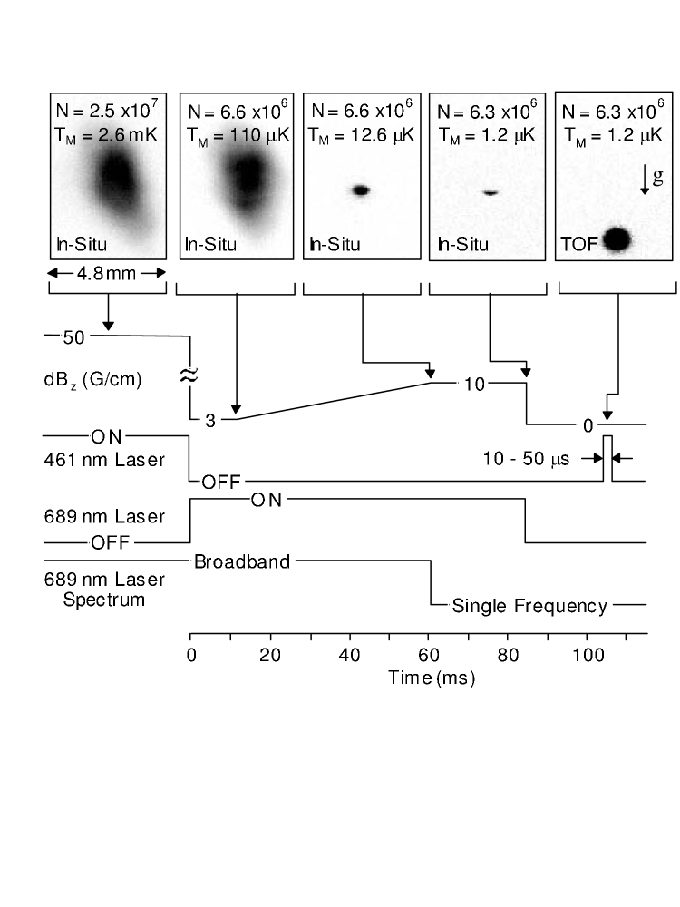
Figure 4 depicts the - MOT loading procedure Katori3 . As outlined above, 3107 atoms are first pre-cooled to 2.5 mK in a - MOT. (Note that for the remainder of this paper, the - MOT is loaded without the 707 nm and 679 nm re-pumping lasers.) At time t = 0, the 461 nm light and the atomic beam shutter are switched off, dBz is rapidly lowered to 3 G/cm, and red-detuned, broadband frequency modulated 689 nm trapping beams are turned on. 10 ms later and for the following 50 ms, the cloud is compressed by linearly increasing dBz to 10 G/cm. Frequency modulation parameters for the 689 nm trapping beams are set to provide complete spectral coverage of the - MOT Doppler profile and, as shown below, manipulate the cloud size at the end of the magnetic field ramp. Subsequently, at t = 60 ms, the frequency modulation is turned off and the atoms are held in a single-frequency MOT. Overall, as shown by the images at the top of Fig. 4, this process reduces the sample temperature by more than three orders of magnitude while only reducing the cloud population by a typical factor of 3 - 4, giving final temperatures of 1 K and populations of 107. Typical single frequency trap lifetimes and spatial densities are 1 s and 51011 cm-3, respectively.
IV 0 Mechanical Dynamics
As outlined in section I, 0 - MOTs provide a unique opportunity to explore three qualitatively distinct laser cooling regimes whose underlying mechanics are governed by either semiclassical or quantum mechanical physics. In this and the following section, we will describe the unique experimental signatures for regimes (I) - (III) and give detailed explanations for the observed trapped atom behavior.
Insight into regime (I) and (II) thermal-mechanical dynamics is provided by the semiclassical radiative force equation Lett
| (1) | |||||
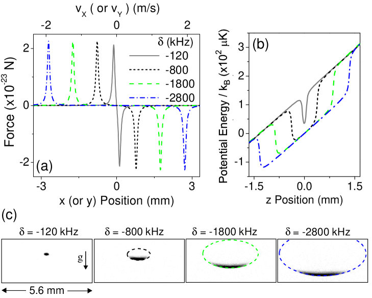
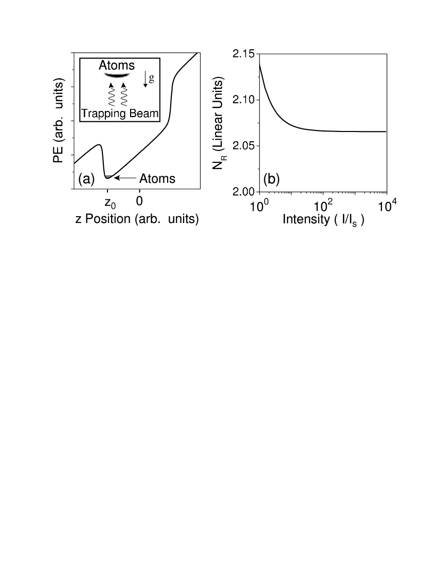
where = , = , and = (/) where = 1.5 () is the state Lande g-factor (Bohr magneton). accounts, along a single axis, for saturation induced by the remaining four trapping beams. Figure 5(a) shows the - radiative force at = = 248 for a range of values while Fig. 6(a) shows the force at = -520 kHz for a range of = values. As described in section I, the qualitative nature of the force and hence the resulting trap mechanical dynamics depends on the relative size of and . For regime (I), corresponding to 120 kHz in Fig. 5(a) or 248 in Fig. 6(a), and the 3D radiative force acts only along a thin shell volume marking the outer trap boundary. Here, the trap boundary roughly corresponds to positions where the radiative force is peaked. This situation, as shown by Figs. 5(b) and 6(b), produces a box potential with a gravitationally induced z-axis tilt. Hence, in the x-y plane, motion consists of free-flight between hard wall boundaries while along the z-axis, mechanical dynamics are set by the relative size of the radiative force “kicks,” gravity, and the cloud thermal energy. As shown in section V, the thermal energy is small compared to the gravitational potential energy. Moreover, the ratio of the maximum radiative force to the gravitational force, 16. Thus, the atoms sink to the bottom of the trap where they interact, along the z-axis, with only the upward propagating trapping beam.
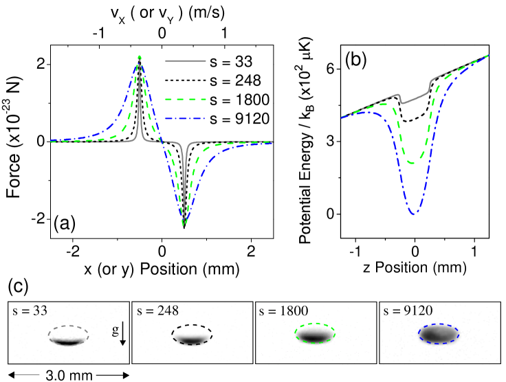
As decreases in Fig. 5(a) or increases in Fig. 6(a), the trap mechanically evolves to regime (II) where produces a linear restoring force and hence, damped harmonic motion Lett ; JILA1c . Consequently the trap potential energy assumes the U-shaped form familiar from standard broad line Doppler cooling. As the trap moves more fully into regime (II), perturbations to the potential energy due to gravity become less pronounced. One expects, therefore, that the cloud aspect ratio will evolve toward the 2:1 value set by the quadrupole magnetic field.

The intuitive descriptions developed above are directly confirmed by Figs. 5(c) and 6(c) which show in-situ images of the - MOT along with overlaid maximum force contours calculated from Eq. 1. For excitation conditions corresponding to regime (II), the cloud approaches the 2:1 quadrupole magnetic field aspect ratio. In contrast, for regime (I) the cloud x-y width is determined largely by the separation between x-y force maxima or alternatively, by the wall separation for the x-y potential energy box. In the vertical direction, the atoms sink to the bottom of the trap where the lower cloud boundary is defined by the location of the z-axis potential energy minima which is, in turn, proportional to the position where the Zeeman shift matches the laser detuning. As increases, shifts vertically downward, an effect predicted in Fig. 5(b) and clearly revealed in Fig. 5(c). To quantify this relationship, Fig. 7 shows versus along with a linear fit to the data giving dz0/d = 2/(dBz) = 0.509(4) m/kHz, in agreement at the 5 level with the expected linear slope of 0.478(2) m/kHz.
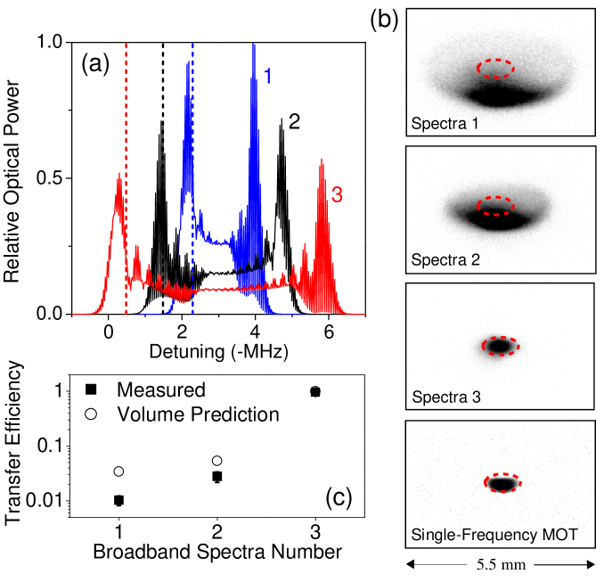
Unique - MOT mechanical dynamics are also manifest in the transfer between the broadband and single-frequency cooling stages. Here, it is important to note that following broadband cooling, the cloud vertical and horizontal 1/e2 radii (rz and rh, respectively) are set by the final value for dBz and the spectral separation between the blue edge of the modulation spectrum and the - resonance. Figure 8(a) shows three typical modulation spectra while Fig. 8(b) shows in-situ images of the corresponding broadband cooled clouds at the end of the magnetic field ramp. For each, the measured temperature is 8.5(0.8) K. Overlaid dashed lines give the maximum force contour for the subsequent = -520 kHz, = 75 single-frequency MOT shown in the bottom frame. Here, dynamics similar to Fig. 5 are observed: as the broadband modulation moves closer to resonance, the cloud density distribution becomes more symmetric and the aspect ratio evolves toward 2:1. Figure 8(c) shows the broadband to single-frequency MOT transfer efficiency TE versus broadband spectra number. Clearly, TE increases as the overlap between the broadband cooled cloud and the single-frequency MOT force contour increases, indicating that TE can be optimized by “mode-matching” rz and rh to the single-frequency MOT box. This idea is supported by open circles in Fig. 8(c) which give predicted TE values based on the relative volume of the broadband cooled cloud and the single-frequency radiative force curve. Overall, the prediction reproduces observed TE values with a discrepancy for spectra 1 and 2 that likely arises from the broadband MOT density distribution.
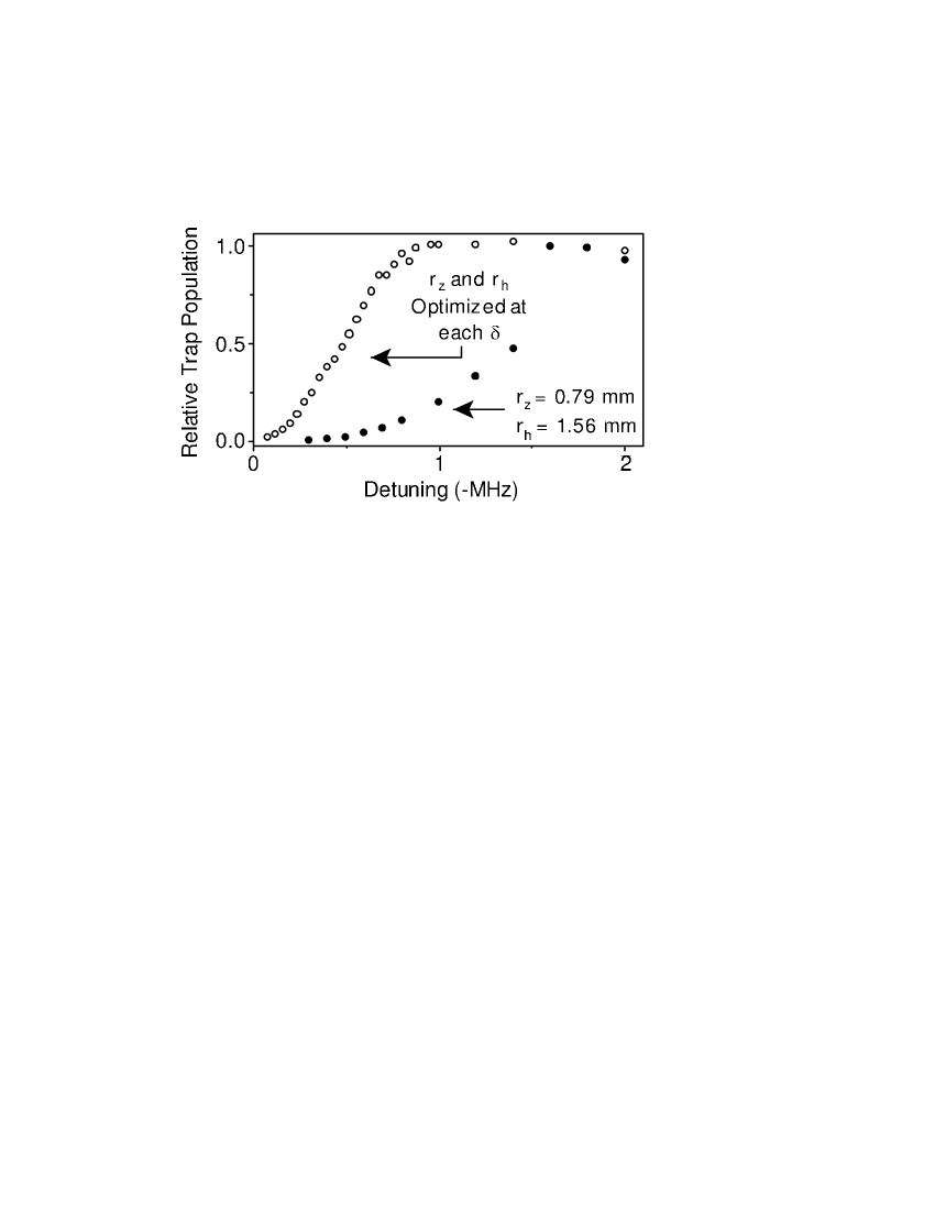
Further evidence for broadband to single-frequency mode-matching is provided by the single-frequency MOT population N versus shown in Fig. 9. Here, solid circles give N versus when rz = 0.79 mm and rh = 1.56 mm. According to the Fig. 5 model, the single-frequency MOT acquires these dimensions at = -1637 kHz, which lies within 2 of the value where N is peaked. Hence, we again find that optimal transfer occurs when rz and rh are matched to the single-frequency radiative force contour. Additional confirmation for this effect is provided by open circles in the figure which give N when rz and rh are optimized at each . To understand the trend in this case toward smaller N as decreases, note the non-zero slope for the blue edge of the modulation spectrum sets the minimum effective detuning that can be used during the broadband cooling phase. In analogy to Fig. 5, sets minimum values for rz and rh. Thus mode-matching becomes progressively more difficult as decreases and the single-frequency radiative force contour shrinks, leading to the observed decrease in N.
V 0 Thermodynamics
0 - MOTs display a rich variety of thermodynamic behaviors that are directly linked to the mechanical dynamics explored in section IV. Figure 10(a) shows the MOT equilibrium temperature TM versus for saturation parameters ranging from = 7.5 to = 1800. For large and , corresponding to regime (I), , TM is basically -independent. Insight into this behavior is provided by Fig. 11(a), which details the unique regime (I) connection between trap thermodynamics, the spatial dependence of the radiative force, and the relative size of the radiative force and gravity. Recall that for , the cloud sags to the bottom of the trap where interactions occur, along the vertical z-axis, with only the upward propagating trapping beam. Moreover, due to polarization considerations and the free-flight motion executed by atoms in the horizontal plane, horizontal beam absorption rates are more than 4 smaller than the vertical rate. Trap thermodynamics, therefore, are dominated by a balance between gravity and the radiative force due to the upward propagating beam. Here, it is important to realize that as changes, the z-axis atomic position self adjusts such that the effective detuning, - dB, remains constant. Consequently the trap damping and diffusion coefficients, and thus the equilibrium temperature, remain constant.
To obtain a quantitative expression for TM under these conditions, we first find the damping coefficient by Taylor expanding
| (2) | |||||
where (/) = is evaluated at = 0, z = . Solving = 0 and using = (/), the -independent effective detuning is given by
| (3) |
which, in combination with Eq. 2, states that the scattering rate depends only on , , and . Substituting this expression into (/), we obtain the damping coefficient
| (4) |
Next, the diffusion coefficient is calculated by substituting Eq. 3 into the single-beam scattering rate. is then given by
| (5) |
Combining Eqs. 4 and 5, the predicted -independent equilibrium temperature is
| (6) | |||||
where we have used for 1. As shown by Fig. 11(b), the numerical factor is approximately 2 over the entire relevant experimental range. Regime (I) temperatures, therefore, depend only on . To test this prediction, Fig. 10(b) shows TM versus for a fixed large detuning = -520 kHz. For the central portion of the plot where regime (I) dynamics are relevant, we find good agreement with Eq. 6.
For small in Fig. 10(a), the system evolves from regime (I) to regime (II) where , . As this transition occurs, trap dynamics change from free-flight to damped harmonic motion. Here, one expects thermodynamics similar to ordinary Doppler cooling including - and -dependent minima with equilibrium values having the functional form Lett ; JILA1c
| (7) |
where , realized at = /2, is a generalized version of the 1 Doppler limit. As shown by the solid lines in Fig. 10(a), Eq. 7 correctly reproduces the functional shape of the data. As shown by Fig. 10(c), however, matching the absolute data values requires multiplying Eq. 7 by a -dependent global scaling factor ( 1) whose value decreases with , leading to temperatures well below the standard Doppler limit . In contrast to ordinary Doppler cooling, the cloud thermal energy in regime (II) is thus not limited by half the effective energy width of the cooling transition. Notably, we find this surprising result cannot be explained either by analytic treatments of Eq. 1 or semiclassical Monte-Carlo simulations of the cooling process. The Monte-Carlo simulations, in fact, simply reproduce standard Doppler theory. Finally, as approaches unity in Fig. 10(b), the trap enters regime (III) where kBT/ and thus the cooling becomes fully quantum mechanical. Here, we obtain a minimum temperature of 250(20) nK, in good agreement with the quantum mechanically predicted value of half the photon recoil temperature /2 = /kB = 230 nK dalibard89 .
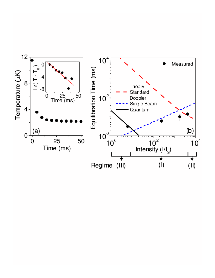
The approach to thermal equilibrium also displays signatures of regimes (I) - (III). Figure 12(a) gives the cloud temperature versus time for a = -520 kHz, = 248 single-frequency MOT. As shown by the figure inset, the data is well fit by a single exponential aside from the rapid decrease for times 5 ms that arises from atoms falling outside the trap capture velocity Curtis ; PTB . Recall from Fig. 10 that scanning at this detuning provides access to all three cooling regimes, each of which is characterized by a unique evolution toward thermal equilibrium. Specifically, for regimes (I) and (II), semiclassical Doppler theory predicts and equilibration time = /2 where is given in regime (I) by Eq. 4 and, according to ordinary Doppler theory, in regime (II) by Lett ; JILA1c
| (8) |
Conversely, quantum theory predicts that for regime (III), follows dalibard89
| (9) |
where is the initial cloud temperature. As a test of these predictions, Fig. 12(b) shows versus at = -520 kHz along with values predicted by the above three theories. Note that for each value we find the temperature versus time is well fit by a single exponential aside from the 5 ms long rapid decrease typified by Fig. 12(a). In regime (II) at = 4520, = 14(2) ms, in good agreement with Doppler theory which gives 12 ms. As expected for regime (I), corresponding to 10 s 4000, follows equilibration times predicted by the single-beam damping coefficient while in regime (III) at = 6.1, = 3.1(4) ms, consistent with the Eq. 9 quantum mechanical predictions.
VI 0 Cooling and Momentum-Space Crystals
Tuning to 0 during the single-frequency cooling stage reveals two fundamental and unique physical processes: (1) the creation of well-defined momentum packets whose velocity space alignment mimics lattice points on a face-centered cubic crystal and (2) laser cooling around a velocity where the radiative force balances gravity. In the following, we explore these two effects in detail.
Basic insight into 0 momentum packet formation can be obtained by considering the elementary problem of 1D atomic motion in the presence of two counter-propagating 0 light fields. For simplicity, we assume = 0. According to Eq. 1, an atom with initial velocity will preferentially interact with the field for which 0. Hence, the absorption process preferentially accelerates rather than decelerates the atom, further decreasing the probability for absorption events that slow the atomic motion and enabling ”positive feedback” in velocity space. This process terminates for final velocities satisfying
| (10) |
which has a linear dependence and scales with . Neighbor atoms with initial velocities around undergo similar ”positive feedback” acceleration and ultimately achieve final velocities near . To quantify this latter effect, we first simplify the problem by neglecting the beam for which 0. The equation of motion for the atomic velocity is then
| (11) |
which can be solved analytically for the interaction time as a function of the velocity
| (12) | |||||
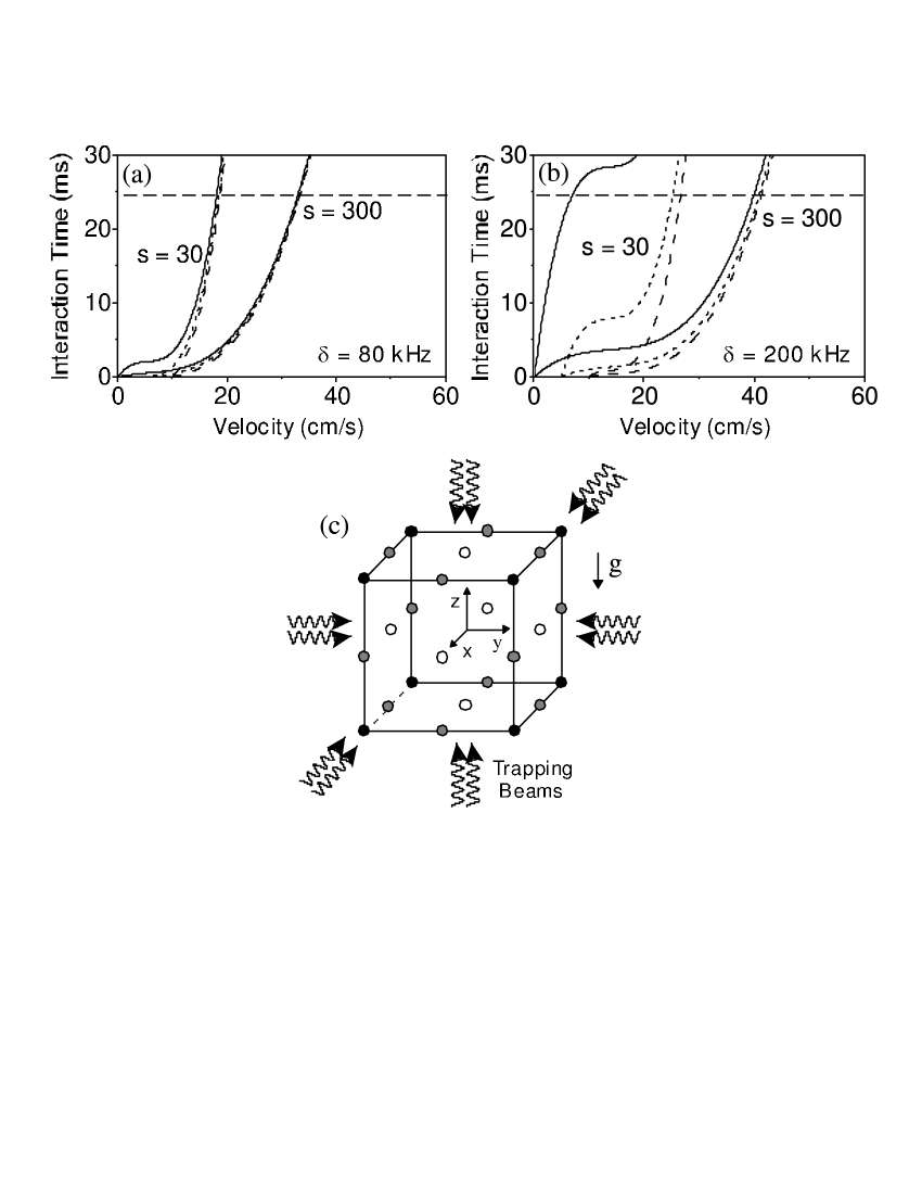
Figures 13(a) and 13(b) show plots of Eq. 12 at = 80 kHz and = 200 kHz, respectively. For both, = 30 or = 300. The chosen values of 0.1 cm/s, 5 cm/s, and 10 cm/s span the velocity distribution for a 12 K cloud. Assuming an interaction time of 25 ms, Fig. 13(a) clearly shows that due to laser induced acceleration, the entire range of initial velocities is rapidly bunched to a significantly reduced range of final velocities. Considering a fully 1D situation, this result implies the cloud is divided into two well defined and oppositely moving packets. As increases to 200 kHz in Fig. 13(b), the = 30 atom-light interaction becomes sufficiently weak for 0 that two final velocity groups centered around 8 cm/s and 25 cm/s appear. In contrast, we find that for = 300 the transition to two groups does not occur until 400 kHz. Accounting again for the full 1D symmetry, the = 30 case corresponds to dividing the = 0 cloud into three groups, two that move in opposite directions with relatively large final velocities and one that, in comparison, is nearly stationary. Overall, Eq. 11 thus predicts that for 0 the atomic cloud evolves into a discrete set of momentum-space packets. As decreases at fixed , the number of packets increases while, as predicted by Eq. 10, the mean velocity for a given packet scales with both and .
Generalizing this analysis to the full 3D molasses beam geometry leads to the structure shown in Fig. 13(c): a 3D array of momentum-space groups whose alignment mimics the lattice points on a face-centered-cubic crystal. From symmetry considerations, cube corners correspond to three beam interactions in which the cloud is divided into two pieces along each coordinate axis. From Figs. 13(a) and 13(b), these points have a - and -dependent mean velocity and appear at relatively small detunings. For larger values, two-beam interactions fill points along the Fig. 13(c) corner connecting lines. In analogy to = 30 in Fig. 13(b), atoms in these points have 0 along a single axis and thus remain nearly stationary. Along the remaining two axes, however, 0, enabling acceleration to larger . The 3-beam to 2-beam transition, as shown in Figs. 13(a) and 13(b), occurs at progressively larger values as increases. Together, the two processes form a total of 20 divided groups with 8, 4, and 8 packets in the top, middle, and bottom layers of the cube, respectively. Finally, as increases further, atoms with 0 along two axes experience acceleration only along a single axis, producing the 1-beam lattice points shown as 6 open circles in the Fig. 13(c) cube face centers.
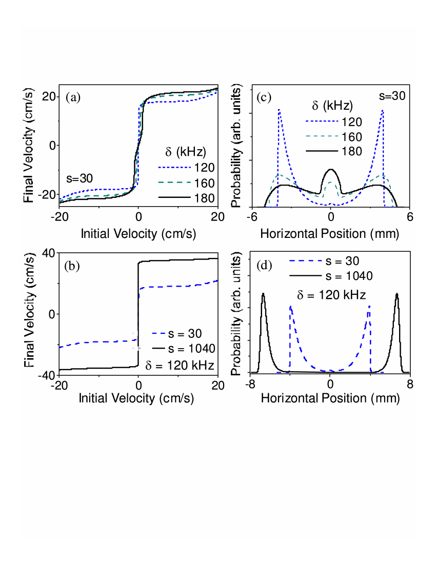
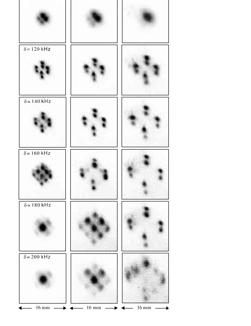
Figure 14 shows an array of top view (slightly off vertical) in-situ cloud images for intensities ranging from = 30 to = 1040 and detunings spanning = 80 kHz to = 200 kHz. For each, = 0 and the atom-light interaction time is fixed at tH = 25 ms (tV = 25 ms) in the horizontal x-y plane (along z-axis) molasses beams. The initial tH = tV = 0 cloud temperature is 11.5(2) K. Here, the observed cloud evolution agrees well with the qualitative predictions developed from the Fig. 13 model. As increases at fixed , sets of n-beam lattice points sequentially fill with n = 3 filling first followed by n = 2,1. Moreover, as increases, transitions between the n-beam processes occur at progressively larger values. Finally, for fixed , the mean lattice point velocity, proportional to the resulting lattice point spacing in the Fig. 14 images, scales with as expected from both Eq. 10 and Fig. 13. Note that qualitatively similar dynamics are observed for 0. The detailed changes to the cloud evolution that result from this situation are described below.
The intuitive understanding of 0 dynamics developed above is confirmed by Fig. 15. Here, we show numerical calculations based on Eq. 1 of the final horizontal velocity and spatial distributions for the = 30 column and = 120 kHz row in Fig. 14. For the calculations, = 0, tH = 25 ms, and the initial cloud temperature is 11.5 K. The Figs. 15(c) and 15(d) spatial distributions should be compared to cube lines in the x-y plane along the Fig. 14 x-y molasses beam propagation directions. Importantly, this fully 1D model reproduces both the Fig. 14 observations and the Fig. 13 predictions for the - and -dependent lattice point filling factors and mean lattice point velocity. As expected, the temperature of each packet in its moving frame is lower than the tH = tV = 0 ms atomic cloud, a result arising from the previously described velocity bunching effects and directly connected to cloud shape asymmetries observed in both the experiment (note the sharp outer cloud edges) and the Fig. 15 theory. Notably, however, only two vertical layers are observed in Fig. 14 while the Fig. 13 model predicts three. As explained below, this apparent discrepancy arises from novel gravitationally induced z-axis dynamics.
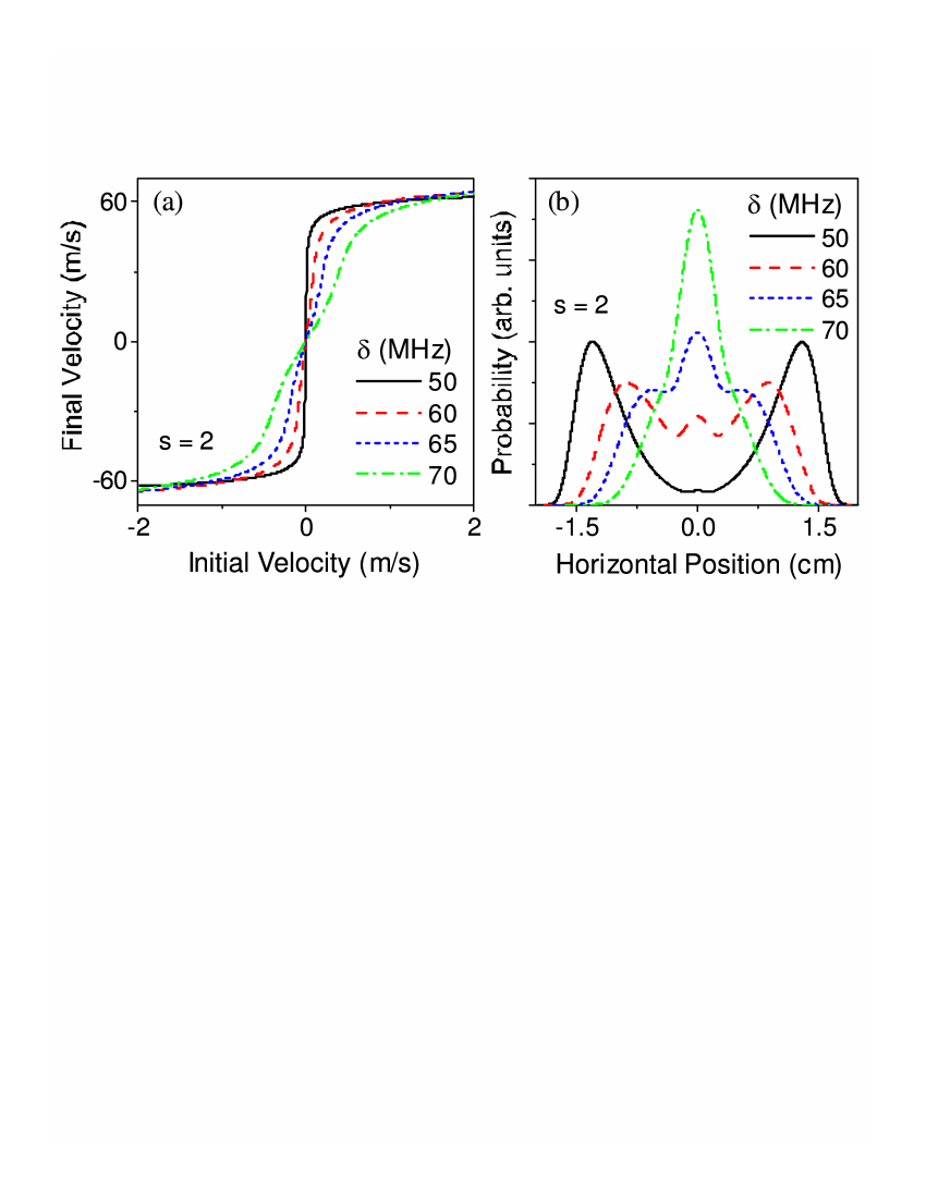
At this point, it is important to realize that Eq. 1 is semiclassical and thus does not account for dynamics that depend on the relative size of and . The 0 momentum crystals observed here, therefore, are a universal feature of Doppler limited systems. Similar processes should then occur with broad lines such as the 461 nm - transition. To test this possibility, Fig. 16 shows numerically simulated final horizontal velocity and spatial distributions for a 2.5 mK 88Sr cloud excited by 461 nm 0 optical molasses. For the calculation, = 0, tH = 500 s, and = 2. As clearly indicated by the figure, structures very similar to those shown in Fig. 14 can be generated over length scales consistent with 461 nm cooling beam diameters and typical - MOT temperatures. Moreover, we find that by increasing either or tH, structures with contrast identical to those shown in Figs. 14 and 15 can be created. Note the model does not account for spontaneous emission induced random walk heating, a process the would tend to smear the contrast between individual momentum packets. This omission, however, should not significantly affect Fig. 16 since random walk heating scales as Lett while, from Eq. 1, the directional acceleration scales as . Thus, as increases from the narrow to the broad line case, random walk heating becomes progressively less important.
Although the physics underlying 0 momentum-space crystals is thus fully operative for broad lines, details of the crystal formation process will make experimental observations difficult. From Eq. 10, for a given packet is proportional to . Hence, broad line packet velocities are orders of magnitude larger than those achieved in the narrow line case. In Fig. 16, for example, 60 m/s. Visualizing the entire structure then requires imaging light with an optical bandwidth of 260 MHz or an equivalently broad optical transition. This situation should be compared to the experiments performed here where 1 m/s, and hence sufficient imaging bandwidth is obtained with the /2 = 32 MHz - transition. In addition, sets the lattice point spacing, or alternatively the molasses beam diameter, required to achieve a given contrast between individual lattice points. For the contrast shown in Figs. 14 and 15, for example, the required broad line molasses beam diameters grow to tens of centimeters, making experimental observations impractical.
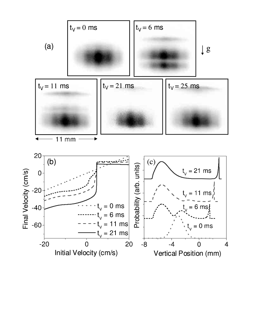
Figure 17(a) shows in-situ images of the 689 nm 0 molasses when the cloud is viewed in the horizontal x-y plane at 45o to the x-y axes. For the images, = 0, = 30, = 140 kHz, tH = 25 ms, and tV is varied from tV = 0 ms to tV = 25 ms. Here, the apparent contradiction between Fig. 14 and the Fig. 13(c) prediction for the number of vertical layers is shown to occur due to gravity induced dynamics. Increasing tV from tV = 0 ms to tV = 6 ms, for example, creates three vertical layers, as predicted by Fig. 13(c). For tV 6 ms, however, the lower two layers slowly merge together, becoming a single cloud along the vertical direction for tV 21 ms. To understand this process, recall that the central layer in the Fig. 13(c) cube corresponds to atoms with near zero z-axis velocities. For the chosen and in the absence of gravity, therefore, these atoms would remain near = 0. As shown by the numerical calculations in Figs. 17(b) and 17(c), however, gravity accelerates the central layer into resonance with the downward propagating molasses beam, causing the two downward propagating layers to merge. For the tV = 25 ms time used in Fig. 14, this process is complete. Hence, only two layers are observed with the more (less) intense packets in the Fig. 14 images corresponding to the lower two (uppermost) cube layers.
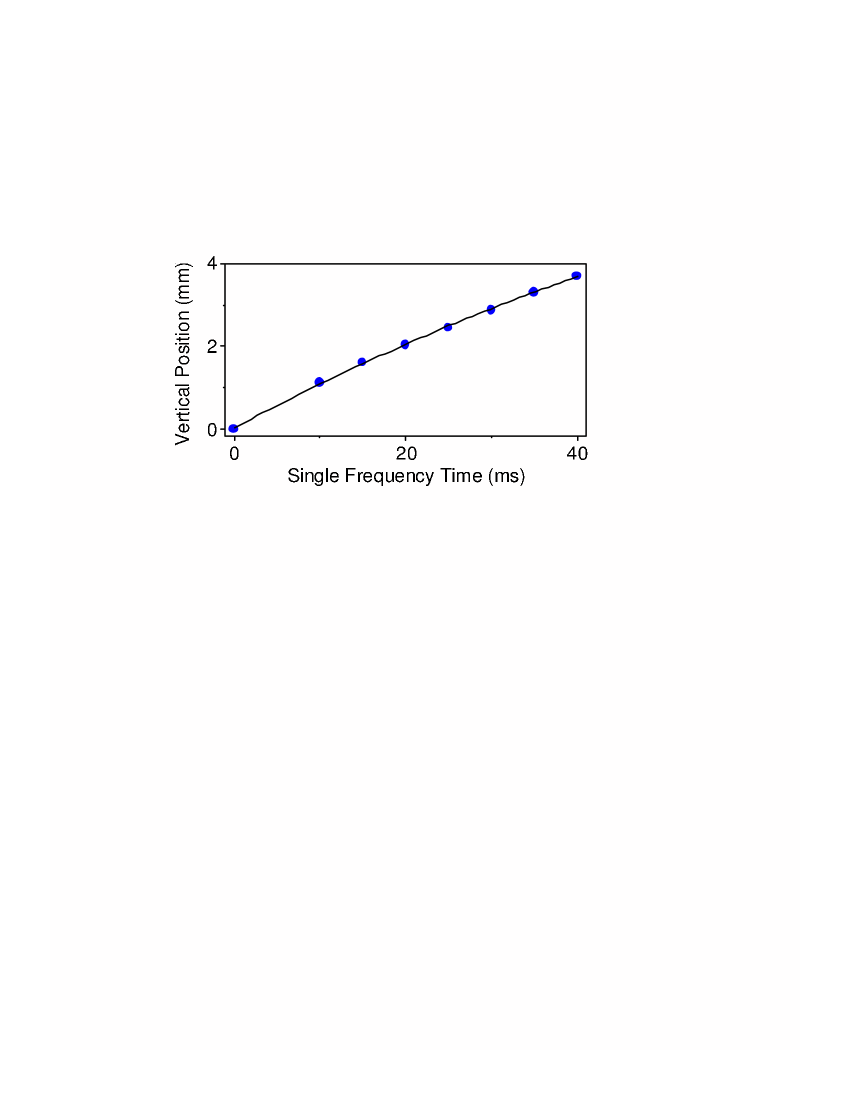
Comparing the numerically simulated 0 spatial distributions with Figs. 14 and 17(a) reveals that theoretically predicted = 0 lattice spacings are 2 larger than observed. This result occurs due to stray magnetic fields. Here, an independently measured 100 mG/cm permanent chamber magnetization spatially shifts the effective detuning as the atoms move outward, causing an apparent deceleration and thus reduced lattice spacing. This effect can be seen most clearly by measuring the vertical position of the upward moving cube layer versus tV. For the upward moving layer, Eq. 1 predicts that the atoms are accelerated to a velocity where the radiative force balances gravity. The cloud then moves upward at and hence, experiences an effective acceleration = 0. To test for a magnetic field induced non-zero , Fig. 18 shows versus tV for = 30 and = 140 kHz. The solid line in the figure is a fit to the simple kinematic equation = - . Here, is treated as an initial velocity since for = 30 and = 140 kHz, the atoms are accelerated to in 2 ms. From the fit, we find = -0.98(16) m/s2, consistent with a stray gradient dBz = 100 mG/cm. Once this gradient is included in numerical calculations of Eq. 1, the measured and calculated lattice point spacings agree.
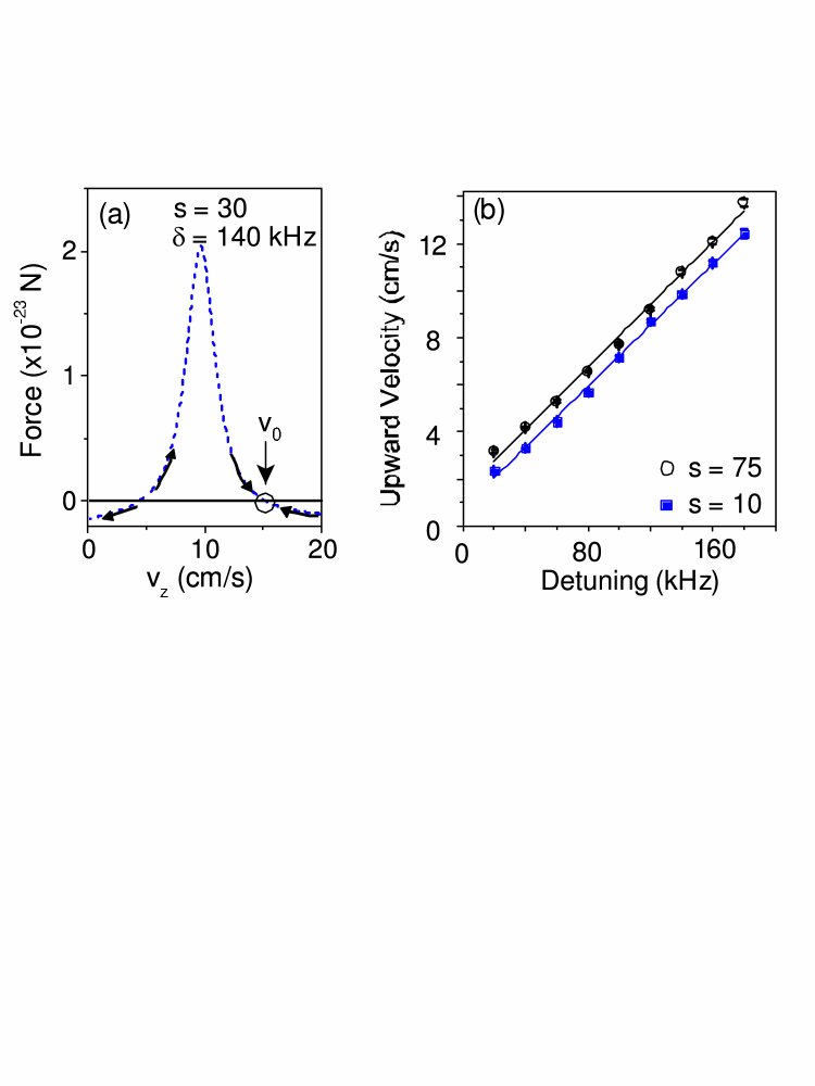
Finally, the exceptionally sharp velocity and thus spatial distributions for the upward propagating layer in Fig. 17 imply velocity compression beyond the bunching effects described earlier. In fact, as shown by Fig. 19(a) which depicts the composite gravitational and radiative force for the upward moving atoms, stable cooling occurs around where the composite force is zero. From Eq. 2, is given by
| (13) |
which depends linearly on and scales approximately as . Fig. 19(b) shows measured values for versus at = 10 and = 75, clearly demonstrating the expected linear -dependence. To obtain quantitative comparisons with theory, we next perform linear fits to the data and then obtain predicted values for from numerical calculations that include the 100 mG/cm field gradient discussed above. From the experiment, we find (/) = 644(17) m/(kHz-s) at s = 10 and 634(19) m/(kHz-s) at s = 75. These slopes agree at the 10 level with the predicted values of (/) = 572(5) m/(kHz-s) at s = 10 and 638(20) m/(kHz-s) at s = 75. Moreover, experimentally observed absolute values for are reproduced by the calculations at the level of 20, in good agreement with the expected Eq. 13 intensity dependence.
The equilibrium temperature of the upward moving layer can be calculated by following the same procedure used to derive Eq. 6. Here, however, we set = 0 in Eq. 2 and perform the Taylor expansion about = . The -independent effective detuning is then
| (14) |
which leads to damping and diffusion coefficients identical to Eq. 4 and 5, respectively. Hence, the expected equilibrium temperature is given by Eq. 6. Thus, gravity, via the ratio , again plays an important role in narrow line thermodynamics, in this case enabling 0 cooling. Unfortunately, this prediction cannot be accurately verified due to spatial overlap among the horizontal plane packets in the upward moving cube layer. The observed and theoretically predicted sharp vertical spatial distributions in Figs. 17(a) and 17(c), however, strongly suggest that 0 cooling is operative in the experiment. Finally, note that although this same cooling mechanism should occur for broad lines where 105, in this case has impractical values on the order of 100 m/s. Moreover equilibrium temperatures are large, at roughly 160(/2) 200 mK for the - transition even at = 1.
VII Conclusions
In summary, narrow line laser cooling exhibits a wealth of behaviors ranging from novel semiclassical dynamics wherein gravity can play an essential role to quantum mechanically dominated sub-photon recoil cooling. In the 0 semiclassical case, trap dynamics are set by either hard wall boundaries or a linear restoring force. Qualitative differences between these two situations are reflected in both the atomic motion and the equilibrium thermodynamics. Here, mechanical dynamics range from free-flight in a box potential to damped harmonic oscillation. Accordingly, equilibrium temperatures range from detuning independent values scaled by the power-broadened transition linewidth to detuning dependent minima well below the standard Doppler limit. As the saturation parameter approaches unity, the trap enters a quantum mechanical regime where temperatures fall below the photon recoil limit despite the incoherent trapping beam excitation. For 0, the cloud divides into momentum-space crystals containing up to 26 well defined lattice points and the system exhibits 0 gravitationally assisted cooling. These surprising 0 behaviors, which again occur due to an incoherent process, are theoretically universal features of Doppler limited systems. Observations should therefore be possible, although difficult, with broad line optical molasses. Perhaps a similar 0 mechanical evolution also occurs for atoms, such as the more typically employed Alkali metals, that support both Doppler and sub-Doppler cooling.
The authors wish to thank K. Hollman and Dr. R. J. Jones for their work on the femto-second comb measurements. This work is funded by ONR, NSF, NASA, and NIST.
References
- (1) H. Katori, et al, Phys. Rev. Lett. 82, 1116 (1999).
- (2) R. Maruyama, et al, Phys. Rev. A 68, 011403(R) (2003).
- (3) X.-Y. Xu, et al, Phys. Rev. Lett. 90, 193002 (2003).
- (4) Y. Takasu, et al, Phys. Rev. Lett. 91, 040404 (2003).
- (5) T. Ido and H. Katori, Phys. Rev. Lett. 91, 053001 (2003).
- (6) M. Takamoto and H. Katori, Phys. Rev. Lett. 91, 22301 (2003).
- (7) H. Katori, et al, Phys. Rev. Lett. 91, 173005 (2003); T. Mukaiyama et al, Phys. Rev. Lett 90, 113002 (2003); T. Ido, Y. Isoya, and H. Katori, Phys. Rev. A 61, 061403(R) (2000).
- (8) E. A. Curtis, C. W. Oates, and L. Hollberg, J. Opt. Soc. Am B 20, 977 (2003).
- (9) G. Wilpers, et al, Phys. Rev. Lett. 89, 230801 (2002); T. Binnewies et al, ibid 87, 123002 (2001).
- (10) T. H. Loftus, et al, Phys. Rev. Lett., in press (2004).
- (11) See, for example, H. J. Metcalf and P. van der Straten, Laser Cooling and Trapping (Springer-Verlag, New York, 1999) and references therein.
- (12) P. D. Lett, et al, J. Opt. Soc. Am. B 6, 2084 (1989).
- (13) D. J. Wineland and W. M. Itano, Phys. Rev. A 20, 1521 (1979).
- (14) Y. Castin, H. Wallis, and J. Dalibard, J. Opt. Soc. Am B 6, 92046 (1989); H. Wallis and W. Ertmer, ibid 6, 2211 (1989).
- (15) X.-Y. Xu, et al, Phys. Rev. A 66, 011401(R) (2002).
- (16) This analogy is not rigorously correct since face-centered-cubic crystals lack the lattice points along corner-connecting lines that are observed in the experiment.
- (17) A. Noble and M. Kasevich, Rev. Sci. Instrum. 65, 9 (1994).
- (18) T. E. Barrett, et al, Phys. Rev. Lett. 67, 3483 (1991).
- (19) M. Bode, et al, Opt. Lett. 22, 1220 (1997).
- (20) M. Yasuda and H. Katori, Phys. Rev. Lett. 92, 153004 (2004).
- (21) T. Loftus, et al, Phys. Rev. A 61, 051401(R) (2000).
- (22) T. P. Dinneen, et al, Phys. Rev. A 59, 1216 (1999).
- (23) X.-Y. Xu, et al, J. Opt. Soc. Am. B 20, 968 (2003).
- (24) T. Loftus, J. R. Bochinski, and T. W. Mossberg, Phys. Rev. A 66, 013411 (2002).
- (25) H. Katori, et al, in Atomic Physics XVII, edited by E. Arimondo, P. DeNatale, and M. Inguscio, AIP Conf. Proc. No. 551 (AIP, Melville, NY, 2001), p. 382.
- (26) T. Loftus, et al, in Laser Spectroscopy: Proceedings of the XVI International Conference, edited by P. Hannaford, A. Sidorov, H. Bachor, and K. Baldwin (World Scientific, River Edge, NJ, 2004), p. 34.
- (27) S. B. Nagel, et al, Phys. Rev. A 67, 011401(R) (2003).
- (28) D. P. Hansen, J. R. Mohr, and A. Hemmerich, Phys. Rev. A 67, 021401(R) (2003).
- (29) A. Derevianko, et al, Phys. Rev. Lett. 90, 063002 (2003).
- (30) V. Kokoouline, R. Santra, and C. H. Greene, Phys. Rev. Lett. 90, 253201 (2003).
- (31) R. Santra, and C. H. Greene, Phys. Rev. A 67, 062713 (2003).
- (32) A. Avdeenkov and J. L. Bohn, Phys. Rev. A 66, 052718 (2002).
- (33) H. J. Lewandowski, et al, J. Low Temp. Phys. 132, 309 (2003).
- (34) J. Stuhler, et al, Phys. Rev. A 64, 031405 (2001).
- (35) R. W. P. Drever, et al, Appl. Phys. B: Photophys. Laser Chem. 31, 97 (1983).
- (36) R. J. Jones, I. Thomann, and J. Ye, Phys. Rev. A 69, 051603(R) (2004).
- (37) See J. Ye, et al, J. Opt. Soc. Am. B 20, 1459 (2003) and K. W. Holman, et al, Opt. Lett. 29, 1554 (2004), and references therein.