Importance of small earthquakes for stress transfers and earthquake triggering

Abstract

We estimate the relative importance of small and large earthquakes for static stress changes and for earthquake triggering, assuming that earthquakes are triggered by static stress changes and that earthquakes are located on a fractal network of dimension $D$. This model predicts that both the number of events triggered by an earthquake of magnitude $m$ and the stress change induced by this earthquake at the location of other earthquakes increase with $m$ as $\sim 10^{Dm/2}$. The stronger the spatial clustering, the larger the influence of small earthquakes on stress changes at the location of a future event as well as earthquake triggering. If earthquake magnitudes follow the Gutenberg-Richter law with $b>D/2$, small earthquakes collectively dominate stress transfer and earthquake triggering, because their greater frequency overcomes their smaller individual triggering potential. Using a Southern California catalog, we observe that the rate of seismicity triggered by an earthquake of magnitude $m$ increases with $m$ as $10^{\alpha m}$, where $\alpha=1.05\pm 0.05$. We also find that the magnitude distribution of triggered earthquakes is independent of the triggering earthquake’s magnitude $m$. When $\alpha\approx b$, small earthquakes are roughly as important to earthquake triggering as larger ones. We evaluate the fractal correlation dimension $D$ of hypocenters using two relocated catalogs for Southern California. The value of $D$ measured for distances $0.1<r<5$ km is $D=1.54$ for the Shearer et al. [2003] catalog and $D=1.73$ for the Hauksson et al. [2003] catalog. The value of $D$ reflects both the structure of the fault network and the nature of earthquake interactions. By considering only those earthquake pairs with inter-event times larger than 1000 days, we can largely remove the effects of short-term clustering. Then $D\approx 2$, close to the value $D=2\alpha=2.1$ predicted by assuming that earthquake triggering is due to static stress. The value $D\approx 2b$ implies that small earthquakes are as important as larger ones for stress transfers between earthquakes, and that considering stress changes induced by small earthquakes should improve models of earthquake interactions.

Agnès Helmstetter, now at Lamont-Doherty Earth Observatory, Columbia University (e-mail: agnes@ldeo.columbia.edu) Yan Y. Kagan, Department of Earth and Space Sciences, University of California, Los Angeles, California. (e-mail: ykagan@ucla.edu) David D. Jackson, Department of Earth and Space Sciences, University of California, Los Angeles, California. (e-mail: djackson@ucla.edu) Helmstetter, Kagan, and Jackson Stress transfers and earthquake triggering Gindraft=false

PostScript file created:

1 Introduction

Large shallow earthquakes are followed by increased seismic activity known as “aftershocks”. Aftershock sequences of small earthquakes are less obvious because the aftershock productivity is weaker, but can be observed after stacking many sequences [Helmstetter, 2003]. Several mechanisms have been proposed to explain earthquake triggering due to the static stress change induced by a prior event: rate-and-state friction [Dieterich, 1994], sub-critical crack growth [Das and Scholz, 1981; Shaw, 1993], viscous relaxation [Mikumo and Miyatake, 1979], static fatigue [Scholz, 1968], pore fluid flow [Nur and Booker, 1972], or simple sand-pile SOC models [Hergarten and Neugebauer, 2002]. Kagan and Knopoff [1987a] proposed that random, Brownian motion-like stress fluctuations cause Omori-law aftershock rate decay. Coulomb stress change calculations have been used to predict the locations, focal mechanisms and times of future earthquakes (see reviews by Harris [1998], Stein [1999] and King and Cocco [2001]). Because large earthquakes modify stress over a much larger area than smaller ones, and because computing Coulomb stress changes requires a good model of slip distribution available only for large earthquakes, most studies have neglected the influence of “small” earthquakes. Most researchers include only the mainshock and its largest foreshock or aftershock to predict the location of future aftershocks. The success of this approach is significant but limited. Only about 60% of aftershocks are located where the stress increased after a mainshock [Parsons, 2002]; stress shadows (proposed decrease of the seismicity rate where Coulomb stress change is negative) are seldom or never observed [Marsan, 2003; Felzer et al., 2003b]; and the correlation of Coulomb stress change with aftershock locations is rather sensitive to the assumed slip distribution [Steacy et al., 2004]. Coulomb stress change from the $M_{W}$ 7.3 Landers earthquake does not explain the triggering of the $M_{W}$ 7.1 Hector-Mine earthquake [Harris and Simpson, 2002] which occurred 7 years after Landers and 20 km away. Several alternative models have been proposed to explain the triggering of the Hector-Mine earthquake: viscoelastic effects [Zeng, 2001], dynamic triggering [Kilb, 2003], or secondary aftershocks [Felzer et al., 2002]. Felzer et al. [2002] suggested that Hector-Mine may have been triggered indirectly by an aftershock of Landers, i.e., secondary aftershocks and small earthquakes may be important for stress triggering.

A few studies have estimated the scaling of the aftershock number with the mainshock magnitude [Solov’ev and Solov’eva, 1962; Papazachos et al., 1967; Utsu, 1969; Singh and Suarez, 1988; Yamanaka and Shimazaki, 1990; Davis and Frohlich, 1991; Molchan and Dmitrieva, 1992; Shaw, 1993; Drakatos and Latoussaki, 2001]. In these studies, the “mainshock” was defined as the largest event of a sequence, and “aftershocks” were then selected in a space-time window around the mainshock. These studies proposed that the number of aftershocks increases exponentially $\sim 10^{\alpha m}$ with the mainshock magnitude $m$, with an exponent $\alpha$ in the range [0.65, 1]. Other researchers [Jones et al., 1995; Michael and Jones, 1998; Helmstetter, 2003; Felzer et al.; 2004] later suggested that the same mechanisms may explain two kinds of triggering: that of aftershocks by a previous larger earthquake and that of a large earthquake by a previous smaller one. Indeed, the distribution of times between an earthquake (“foreshock”) and a subsequent larger earthquake follows the Omori law as for usual aftershocks [Jones and Molnar, 1979], and the magnitude of triggered earthquakes is independent of that for the triggering event [Helmstetter, 2003]. In the work of Helmstetter [2003] and Felzer et al. [2004], “aftershocks” were selected as earthquakes occurring in a space-time window after a “mainshock” (any earthquake not preceded by a larger one), and could be larger than the mainshock. Using different methods (see section 3.4), Helmstetter [2003] found $\alpha=0.8\pm 0.1$ and Felzer et al. [2004] found $\alpha=1$ for Southern California seismicity.

Other studies measured the exponent $\alpha$ using a statistical model of seismicity [Ogata, 1989; Kagan, 1991b; Ogata, 1992; Console et al., 2003; Zhuang et al., 2004], which assumes that any earthquake can trigger other events with a rate which decays in time according to Omori’s law and which increases with magnitude as $\sim 10^{\alpha m}$. Ogata has coined the term“ETAS” for “epidemic type aftershock sequence” to describe this class of models. However, these models are now being used to describe the statistics of all earthquakes, not just aftershocks. Here we will use the designation “ETES” for “epidemic type earthquake sequence”. Optimizing the likelihood of the ETES model gives an estimation of the model parameter $\alpha$. When applied to long-time catalogs, this method usually gives a smaller value of $\alpha$, in the range 0.5-0.7 [Console et al., 2003; Zhuang et al., 2004], than would result by simply counting the number of aftershocks. When applied to individual aftershock sequences [Guo and Ogata, 1997], this method gives from one sequence to another a large variation of $\alpha$, ranging from 0.2 to 1.9 with a mean value of 0.86.

Yamanaka and Shimazaki [1990] explained the value $\alpha=1$ observed for interplate earthquakes by assuming that aftershocks are located on patches of the mainshock fault plane. If the stress drop is independent of magnitude, the density of aftershocks on the fault plane is a constant. Therefore, the number of aftershocks is proportional to the area of the mainshock rupture plane, i.e., $\alpha=1$. Hanks [1992] used the same model to show that, if $\alpha$ is equal to the exponent $b$ of the Gutenberg-Richter (GR) law, small earthquakes are just as important as larger ones in redistributing tectonic forces on faults. Helmstetter [2003] later generalized this model by assuming that earthquakes are located on a fractal network of dimension $D$. This model predicts that stress transfers between earthquakes and earthquake triggering scales as $\sim 10^{Dm/2}$. Therefore, if earthquakes are very clustered in space with $D<2b$, small earthquakes will be more important than larger ones for transferring static stress between events and thus for earthquake triggering.

In this work we revisit the work of Helmstetter [2003] by using a different method to define mainshocks and aftershocks, and by discussing the model in more detail. We then test the model by estimating the fractal correlation dimension $D$ of earthquake hypocenters, using two relocated catalogs for Southern California. We compare the observed value of $\alpha$ with the prediction $\alpha=D/2$ [Helmstetter, 2003].

2 Scaling of stress transfers and earthquake triggering with the mainshock magnitude

We estimate the relative importance of small earthquakes for stress transfers and for earthquake triggering. Our model is based on the following assumptions:

• Earthquakes are triggered by a static stress step induced by the mainshock. Triggering from dynamic stress changes may have a different scaling with magnitude. We also assume that the mainshock does not change the stressing rate, i.e., we neglect the influence of post-seismic viscous relaxation on the seismicity. We do not impose a relation between the number of aftershocks and the stress change; we simply assume that the rate of aftershocks at point $\vec{r}$ at time $t$ after a stress change $\sigma$ is a function which depends only on $t$ and $\sigma$. For instance, in the rate-and-state model [Dieterich, 1994], the instantaneous increase in seismicity rate is proportional to $\exp(\sigma)$, but the total number of aftershocks (integrating over time) is proportional to the stress change.

• A triggered earthquake s size is independent of the magnitude of the triggering event (“mainshock”) as suggested by [Helmstetter, 2003]. This implies that the crust is everywhere close to failure, such that any small earthquake, triggered by a previous small one, can grow into an event much larger than its trigger.

• We consider earthquakes with rupture width smaller than the thickness of the seismogenic crust, for which the rupture length $L$ is proportional to its width $W$.

• The rupture length scales with the seismic moment as $L(M)\sim M_{0}^{1/d}$. For earthquakes smaller than the thickness of the seismogenic crust and for a constant stress drop, $d=3$. For larger earthquakes, several models have been proposed, with $d=1$, $d=2$ or $d=3$ (see Kagan [2004b] for a review).

• Earthquakes are located on a fractal network of dimension $D$. The spatial clustering of seismicity is due both to the geometry of the fault network and to earthquake interactions. Over long time-scales, aftershocks should cover uniformly the active fault network, and thus should share the spatial distribution of the non-correlated background seismicity. In our model, we define $D$ as the fractal dimension of the long-term time-independent seismicity, not including short-term clustering due to earthquake interactions.

For a constant stress drop, the Coulomb stress change at point $\vec{r}$ due to a finite dislocation of length $L$ and width $W\sim L$ depends only on the ratio $r/L$ and the direction $\Phi$ (set of 3 angles) between the rupture plane and the fault plane at point $\vec{r}$ on which we compute the stress [Kagan, 1991c]. This means that the average stress change at a distance $r$ proportional to $L$ from an earthquake of length $L$ is independent of this earthquake’s magnitude. The only difference between small and large events is that larger ones increase the stress over a larger area. We can thus write the stress change (tensor) as a function ${\boldmath\sigma}(r/L,\Phi)$. We first estimate the scaling of stress transfers between quakes as a function of the magnitude of the event which increases the stress. The expectation of the norm of the stress tensor induced by an earthquake of length $L$, integrating over the location of all earthquakes is given by

$$\sigma(L)={\rm E}(||{\bf\sigma}(r/L,\Phi)||)=\int\limits_{\Phi}d\Phi~{}\int\limits_{0}^{\infty}~{}||{\bf\sigma}(r/L,\Phi)||\,p_{r}(r)~{}dr\,,$$ (1)

where $\Phi$ are limits for a set of 3 angles characterizing fault orientation (their exact form depend on the parametrization method) and $p_{r}(r)$ is the time-independent density of earthquakes at a distance $r$ from another earthquake.

For a fractal distribution,

$$p_{r}(r)\sim r^{D-1}~{},$$ (2)

where $D$ is the correlation dimension of earthquake hypocenters. The function $p_{r}(r)$ in (1) describes the long-term spatial distribution of seismicity, not including clustering due to aftershocks. Introducing (2) in (1) and using the new variable $x=r/L$, we have

$$\sigma(L)=L^{D}\int\limits_{\Phi}d\Phi~{}\int\limits_{0}^{\infty}~{}\sigma(x,\Phi)~{}p_{r}(x)~{}dx\,.$$ (3)

The integral in (3) is now independent of the event s length; the only dependence on magnitude is in the factor $L^{D}$. The integral is convergent both in the near field (the stress has a $r^{-1/2}$ singularity close to the crack tip which is integrable) and in the far field if $D<3$ because $\sigma(x)$ decays as $1/x^{3}$ for $x\gg 1$. Assuming that $L\sim M_{0}^{1/3}\sim 10^{0.5m}$ (for a constant stress drop and for $L$ proportional to $W$), we can rewrite the average stress $\sigma(M_{0})$ induced by an earthquake of moment $M_{0}$ at the location of another event (distributed according to $p_{r}(r)$) as [Kagan, 1994]

$$\sigma(M_{0})\sim M_{0}^{D/3}\,.$$ (4)

If earthquakes are distributed uniformly in a volume ($D=3$), or if we compute the integral of the stress change induced by a quake on a volume rather than at the location of other events, then $\sigma(M_{0})\sim M_{0}$. In other words, stress change integrated on a volume is proportional to seismic moment, and is therefore dominated by the largest earthquakes in a catalog if the exponent $\beta$ of the cumulative moment distribution is $\beta<1$ (i.e., $b<1.5$ for magnitudes). In contrast, if we compute the stress changes at the location of other quakes, and if $D\approx 2$, then the increase in the stress change with $M_{0}$ is balanced by the decreased number of events proportional to $M_{0}^{-2/3}$ with seismic moment (equivalent to GR law with $b=1$). In this case $D=3\beta$, small earthquakes are just as important as larger ones for stress transfers between earthquakes.

If earthquake triggering is due to static stress changes, the seismicity rate $N(r,\Phi,t)$ at point $(r,\Phi)$ and time $t$ can be written as a function $f(\sigma,t)$ of the stress change $\sigma$ and of the time $t$ after the stress change. The function $f(\sigma,t)$ describes any physical mechanism of earthquake triggering due to static stress changes, such as rate-and state friction [Dieterich, 1994], sub-critical crack growth [Das and Scholz, 1981; Shaw, 1993], viscous relaxation [Mikumo and Miyatake, 1979], static fatigue [Scholz, 1968], or pore fluid flow [Nur and Booker, 1972]. The cumulative number of earthquakes $N_{\rm aft}(L)$ triggered by an earthquake of length $L$ in the time window [$c$, $T$] is given by the integral over time and space of the seismicity rate

$$N_{\rm aft}(L) = \int\limits_{c}^{T}dt~{}\int\limits_{\Phi}d\Phi~{}\int\limits_{0}^{\infty}~{}f(\sigma,t)~{}p_{r}(r)~{}dr$$ (5)

$$= L^{D}\int\limits_{c}^{T}dt~{}\int\limits_{\Phi}d\Phi~{}\int\limits_{0}^{\infty}~{}f(\sigma,t)~{}p_{r}(x)~{}dx\,.$$

The minimum time $c$ is introduced to avoid the singularity of the seismicity rate at time $t=0$ predicted by some models of stress triggering (e.g., in the case of the rate-and-state model [Dieterich, 1994] when a singularity occurs in the stress field). The maximum time $T$ is needed to regularize the integral at large times for some models which predict an Omori law decay with $p\leq 1$ (but we can take $T=\infty$ in Dieterich’s [1994] model). As for the stress change $\sigma(L)$ in (3), the number of triggered earthquakes depends on magnitude only in the factor $L^{D}$. The scaling of aftershock productivity with the size of the triggering earthquake is the same as for stress transfers. For seismic moment

$$N_{\rm aft}(M_{0})\sim M_{0}^{D/3}\,,$$ (6)

and for magnitude

$$N_{\rm aft}(m)\sim 10^{\alpha m}\quad\rm{with}\quad\alpha=0.5D\,.$$ (7)

The result (7) does not depend on the physical mechanism of earthquake triggering, i.e., on the specific form of the function $f(\sigma,t)$ in (5), but is valid for any model in which aftershock properties (seismicity rate, location, duration of the aftershock sequence) are functions of the static stress change induced by the mainshock, and on the time since the stress change, and have no other dependance on the mainshock magnitude. In the next section, we measure the scaling of the aftershock rate with the mainshock magnitude for Southern California seismicity. We then estimate the fractal dimension $D$ of the spatial distribution of hypocenters in section 5 and compare the results with the model’s prediction (7).

3 Scaling of earthquake triggering with mainshock magnitude: observations for California seismicity

We have measured the average rate of triggered earthquakes (“aftershocks”) following a “mainshock” in Southern California to measure the scaling of the number of triggered earthquakes with the triggering magnitude. We first discuss some potential problems in analyzing aftershock properties. We describe the catalog in section 3.2. We then define “mainshocks” and “aftershocks” and explain our declustering procedure. We present our results on the scaling of earthquake triggering with the magnitude of the triggering event in section 3.4, and findings on the magnitude distribution of triggered earthquakes in section 3.5

3.1 Problems with estimating aftershock properties

Several properties of aftershocks are difficult, if not impossible, to estimate and may be very sensitive to the parameters of the declustering procedure. It is particularly difficult to define the total number of aftershocks. If earthquake triggering follows Omori’s law $\sim 1/t^{p}$, with $p\geq 1$ and without cut-off at short times, there is an infinite number of aftershocks shortly after the mainshock when the seismic network is saturated. These aftershocks are not reported in the catalogs. For $p\leq 1$, there are also infinitely many aftershocks at very long times (between an arbitrary time $T$ following the mainshock up to $t=\infty$) which are mixed up with non-correlated, background quakes. Therefore, we miss most aftershocks if we select earthquakes in seismicity catalogs in a finite time window after the mainshock. Because it is impossible to measure the total number of triggered events, an alternative solution is to measure the rate of aftershocks in a finite time window after the mainshock, when the catalog is complete and before the rate goes back to the constant background level. If the temporal variation in the number of triggered events is the same for all mainshock magnitudes (as expected if the rate of aftershocks depends only on the stress and the time since the stress step), then the scaling of the total number of aftershocks (exponent $\alpha$ in (7)) can be measured from that of the rate of triggered events with the mainshock magnitude.

It is also impossible to distinguish between the “direct” (triggered by the “mainshock” only) and “secondary” aftershocks (triggered by a previous aftershock from the mainshock). Because an earthquake is probably not triggered by a single prior quake, but rather by the cumulative effect of all previous events (with a weight depending on the time, distance and magnitude of this particular quake), it is impossible to tell which earthquake was triggered by which other one. Only a stochastic answer can be obtained, assuming a particular model of earthquake interactions: for example, that earthquakes obey the Epidemic Type Earthquake Sequences (ETES or ETAS) model [ Zhuang et al., 2004]. After estimating the parameters by maximizing the likelihood of the model, Kagan and Knopoff [1976] and later Zhuang et al. [2004] have proposed a method to calculate the probability that an earthquake was triggered by a previous one, or that it was a background event. However, if the number of secondary aftershocks is proportional to the number of direct aftershocks, then we can measure the total (observed) rate of triggered seismicity, including direct and secondary aftershocks, which will have the same dependence on the mainshock magnitude as does the number of direct aftershocks [Helmstetter and Sornette, 2003].

Rather than by fitting a multi-parameter stochastic clustering model, such as ETES model, we have estimated earthquake clustering properties here directly from the earthquake catalog, with some simple selection criteria. Although the ETES type models usually describe earthquake clustering well, using them to determine parameters like $\alpha$ can be problematic. First, the estimates so determined are not very robust, because the model parameters are strongly correlated and poorly resolved. Second, the parameter estimates may be biased. Inevitable errors in magnitude, location, and temporary incompleteness after larger events [Kagan, 2004a] may each bias earthquake statistics by underestimating clustering at short distances and times. Kagan [1991b, see p. 142 and his Eq. 36] argues that the value of $\alpha$ obtained by maximum likelihood inversion of ETES parameters depends on the method used to account for the incompleteness of short-term aftershocks in a catalog. Furthermore, the ETES models generally assume isotropic clustering, whereas earthquakes occur preferentially on spatially clustered faults. Neglecting this spatial clustering can lead to underestimating $\alpha$, because the contribution to the total predicted seismicity rate from all small aftershocks better predicts the location of future aftershocks than does the isotropic contribution from the mainshock. A smaller $\alpha$ gives more weight to smaller earthquakes and therefore better accounts for the following factors: incompleteness of the catalog after a large earthquake, the heterogeneity of the spatial distribution of aftershocks, fluctuations of aftershock productivity, and magnitude errors (see Helmstetter et al. [2004] for more details).

3.2 Data

We used the catalog of seismicity for California provided by the Advanced National Seismic System (ANSS) (available at http://quake.geo.berkeley.edu/anss/catalog-search.html). This catalog merges data from several networks (for this work, essentially Southern and Northern California and Nevada). We used earthquakes larger than a magnitude threshold $m_{d}=2$, within the time window 1980/1/1-2004/10/15, and within the rectangular area $32^{\circ}<\rm{latitude}<37.5^{\circ}$ and $-122^{\circ}<\rm{longitude}<-114^{\circ}$. This zone does not include Long Valley volcanic seismicity. We checked that the catalog is complete for $m\geq 2$ in this area and time period (except at short times after a large earthquake). We removed explosions from the catalog.

When available, for large earthquakes, we used moment magnitudes provided by the Harvard catalog (available at http://www.seismology.harvard.edu/CMTsearch.html, see Ekström et al. [2003] and references therein). Otherwise we used the magnitudes provided by the ANSS catalog (see http://quake.geo.berkeley.edu/ftp/pub/doc/cat5/cnss.catalog.5 for more details). The magnitudes for smaller earthquakes are generally $m_{L}$, or local magnitudes estimated from short-period body waves. Our use of magnitudes other than moment magnitude is a potential problem, because the scaling relationships and simple static stress models we employ are based on the seismic moment, which we assume is simply related to magnitude. Hutton and Jones [1993] show $m_{L}$ is a fairly good unbiased surrogate for moment magnitude in the magnitude range 4.5 to 6, but there may be a significant bias for quakes smaller than 4.5. At this point we have to assume that any bias does not affect the results much, but in the future this assumption needs to be tested using moment magnitudes for smaller earthquakes.

3.3 Selection of mainshocks and aftershocks

The objective of the declustering procedure is to select as mainshocks only events not preceded by any large earthquake; then quakes following mainshocks within a specified time and distance are identified as aftershocks. The space and time windows are chosen in order to minimize the influence of non-correlated earthquakes. There are always arbitrary choices in a declustering procedure, so we tested different values for all adjustable parameters. As a test we also applied this declustering method to synthetic catalogs to estimate the accuracy and lack of bias in results.

Because we want to investigate the temporal decay of triggered seismicity and the scaling of aftershock productivity with the mainshock magnitude, we want a declustering procedure which makes minimal assumptions about the properties of aftershock triggering in time, space and magnitude, without introducing a-priori any scaling of the number of aftershocks or their duration with the mainshock magnitude. We assume that larger earthquakes influence seismicity in a wider area, proportional to the mainshock rupture area [Kagan, 2002a].

Practically, we select as mainshocks any earthquake of magnitude $m_{M}$ not in the influence zone $R_{F}\times T_{F}$ of a previous event of magnitude $m\geq m_{M}-\Delta m$. We use generally $\Delta m=1$. This choice ensures that aftershocks of the foreshock are negligible compared to aftershocks of the “mainshock” because aftershock productivity increases rapidly with the mainshock magnitude. We compute distances between earthquake epicenters, because depth has a larger error than horizontal coordinates. The spatial influence zone $R_{F}$ of a foreshock is defined as

$$R_{F}(m)=\max(D_{F},~{}N_{\rm L,F}\times L(m))\,,$$ (8)

where the constant $D_{F}$ accounts for a location’s accuracy, $L(m)$ is the rupture length [WGCEP, 2003] of an earthquake of magnitude $m$

$$L(m)=0.01\times 10^{0.5m}\quad\rm{(km)}\,,$$ (9)

and $N_{\rm L,F}$ is an adjustable factor. Mainshocks are selected with a rectangular area $32.1^{\circ}<\rm{latitude}<37.4^{\circ}$ and $-121.9^{\circ}<\rm{longitude}<-114.1^{\circ}$ slightly smaller (by $0.1^{\circ}$) than the box used to select foreshocks and aftershocks so as to avoid finite size effects.

We then select as aftershocks of a mainshock all quakes of magnitude $m\geq m_{d}$ in the influence zone $R_{A}\times T_{A}$ of the mainshock, or of a previous aftershock of the mainshock, even if they are larger than the mainshock. The size of a cluster can thus increase with time, due to aftershock diffusion or due to secondary aftershocks, as in Reasenberg [1985]. We use a space window

$$R_{A}(m)=\max(D_{A},~{}N_{\rm L,A}\times L(m))\,.$$ (10)

We use parameters $D_{A}$ and $N_{\rm L,A}$ in (10) generally smaller than the parameters $D_{F}$ and $N_{\rm L,F}$ used to define mainshocks, because we do not want to consider as a mainshock any earthquake influenced by a previous one, and we do not want to include as aftershocks distant quakes mixed with the background. Thus, our declustering method has 7 adjustable parameters: $D_{A}$, $D_{F}$, $N_{L,A}$, $N_{L,F}$, $T_{A}$, $T_{F}$ and $\Delta m$. With our algorithm, a small fraction of earthquakes are considered as aftershocks of several mainshocks. For instance, Landers aftershocks are also considered as aftershocks of a $m=2.8$ earthquake which occurred 6 hours before Landers.

Our method is very similar to the one of Reasenberg [1985], except that we do not require that aftershocks be smaller than the mainshock, and we do not include a priori hypotheses on either the scaling of aftershock productivity with the mainshock or on the temporal decrease of the seismicity rate with time. By contrast, Reasenberg [1985] assumes that aftershock productivity increases as $10^{2m/3}$ and that the rate of aftershocks follows the Omori law with $p=1$.

The main differences between this work and the previous analysis of [Helmstetter, 2003] are that Helmstetter [2003] used a constant value for $R_{F}=50$ km (independent of the foreshock magnitude), Helmstetter [2003] also used $\Delta m=0$, and selected as aftershocks earthquakes in the influence zone of the mainshock only (not in the influence zone of a previous aftershock). We also use here a different catalog from [Helmstetter, 2003] (with different minimum magnitude, space and time windows).

Our definition of triggered events is also very similar to that of Felzer et al. [2004], but the parameters (minimum magnitude, time interval) and the method used to compute $\alpha$ differ. The only difference in the algorithm of aftershock selection is that Felzer et al. [2004] selected aftershocks within the influence zone of either the mainshock or of its largest aftershock, while we select aftershocks in the influence zone of both the mainshock and all its aftershocks. This difference should have only a minor effect, as aftershock diffusion is very weak if there is any at all [Helmstetter et al., 2003]. Secondly, if a mainshock triggers a larger event, most of the following events will occur in the influence zone of the largest earthquake, which generally includes the influence zone of the previous “mainshock”.

3.4 Scaling of earthquake triggering with the magnitude of the triggering events

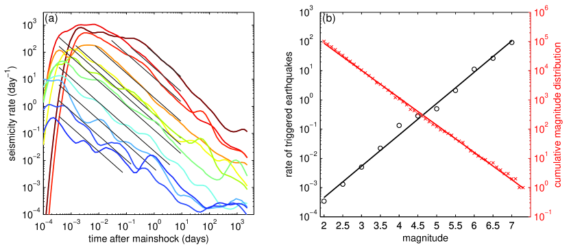
Figure 1: (a) Average rate $\lambda(m_{M},t)$ of $m\geq 3$ earthquakes as a function of the time $t$ after the triggering earthquake, for different values of the magnitude $m_{M}$ of the triggering earthquake increasing from 2 to 7 with a step of 0.5 from bottom to top. The roll-over at short times is due to the incompleteness of the catalog following a strong mainshock. Black lines show the fit of $\lambda(m_{M},t)$ by $K(m_{M})/t^{0.9}$ in the time interval [$t_{\rm min}(m_{M})$, $t_{\rm max}(m_{M})$], where $t_{\rm min}(m_{M})=0.0003$ day (26 sec) for $m_{M}\leq 4.5$ mainshocks. For larger mainshocks $t_{\rm min}(m_{M})$ is estimated using expression (12) as the time when the catalog is complete for $m\geq 3$. The maximum time is either 10 days or the time when the seismicity rate decays below $\lambda_{\rm min}=0.01$ day^-1. (b) Aftershock productivity $K(m_{M})$ as a function of $m_{M}$ (circles) and cumulative magnitude distribution $P(m)$ (crosses). Solid lines are linear regressions of $K(m_{M})$ and $P(m)$ with exponent respectively equal to $\alpha=1.07$ and $b=0.94$.

We stack all aftershock sequences which have the same mainshock magnitude $m_{M}$, for each class of mainshock magnitude ranging from 2 to 7 with a bin size of 0.5. We use a kernel method [Izenman, 1991] to estimate the seismicity rate, by convolving the logarithm of earthquake times with a gaussian kernel of width $h=0.1$ for $m_{d}=2$ and $h=0.2$ for $m_{d}=3$. The results for $D_{F}=3$ km, $D_{A}=2$ km, $N_{L,A}=2$, $N_{L,F}=3$, $T_{F}=1$ yr, $\Delta m=1$ and $m_{d}=3$ are shown in Figure 1. In choosing this parameter, we have checked that our “mainshocks” are almost uniformly distributed in time, and are therefore not strongly influenced by other earthquakes.

For each mainshock magnitude, the aftershock rate decays with the time since the triggering event approximately as

$$\lambda(t,m_{M})={K(m_{M})\over t^{p}}\,,$$ (11)

with $p\approx 0.9$. This expression (11) is only correct in a finite time window [$t_{\rm min}(m_{M})$, $t_{\rm max}(m_{M})$], for which the catalog is complete above $m_{d}$ and the proportion of non-correlated events is negligible. The Omori law has been reported in many observations of aftershock sequences (see Utsu et al. [1995] for a review), and can be derived from several physical models of earthquake triggering. For example, Omori decay (11) with an exponent $p\approx 0.9$ can be reproduced by the rate-and-state model of Dieterich [1994] using a non-uniform stress distribution. Due to our rule of aftershocks and mainshocks selection, the seismicity rate after the mainshock is much larger than before. We conclude that, when Omori law decay with $p\approx 0.9$ is observed, the earthquakes which we define as “aftershocks” are probably causally related to (triggered by) the “mainshock” rather than simply correlated to it.

Based on analyzing the magnitude distribution for several aftershock sequences in Southern California, Helmstetter et al. [2004] have proposed a relation between the magnitude of completeness $m_{c}(t,m_{M})$ as a function of the mainshock magnitude and of the time (in days) since the mainshock

$$m_{c}(t,m_{M})=m_{M}-4.5-0.76\log_{10}(t)$$

$${\rm{and}}\quad m_{c}(t,m_{M})\geq 2.$$ (12)

Earthquakes smaller than this threshold are generally not detected due to overlapping of seismic records and saturation of the network. Of course some fluctuations of $m_{c}$ occur from one sequence to another, but this relation gives a good fit to all sequences we analyzed within $0.3$ magnitude units. For Landers $m=7.3$, expression (12) predicts that the completeness magnitude recovers its usual value $m_{d}=2$ about 10 days after the mainshock.

For each value of $m_{M}$, we fit the rate of aftershocks by (11) with $p=0.9$, in the time interval [$t_{\rm min}(m_{M})$, $t_{\rm max}(m_{M})$], to estimate $K(m_{M})$. The minimum time $t_{\rm min}(m_{M},m_{d})$ is the time after which the catalog is complete for $m\geq m_{d}$, estimated using (12). Parameter $t_{\rm max}(m_{M})$ is either fixed to 10 days or given by the condition $\lambda(t,m_{M})>\lambda_{\rm min}$, where $\lambda_{\rm min}=0.01$ day^-1 is the seismicity rate below which that rate does not obey Omori’s law (11). At large times, the seismicity rate goes to a constant level, due to the background rate or the influence of non-correlated aftershock sequences (see Figure 1). For small $m_{M}$, the seismicity rate increases at large times because the cluster size increases with time, as we enlarge the cluster with new earthquakes related to previous ones. The peak at $t\approx 7$ years for $6\leq m_{M}<6.5$ and $7\leq m_{M}<7.5$ is due to the $M=7.1$ 1999 Hector-Mine aftershock sequence, which is included in the clusters of the 1992 Landers $M=7.3$ and Joshua-Tree $M=6.1$ earthquakes.

Figure 1b shows that aftershock productivity increases exponentially with mainshock magnitude. The value of $K(m_{M})$ (representing the seismicity rate per day for $m\geq m_{d}$ at time $t=1$ day after a mainshock of magnitude $m_{M}$) is given by

$$K(m_{M})=K_{0}~{}10^{\alpha m_{M}}~{}10^{-bm_{d}}~{},$$ (13)

with $K_{0}=0.0033$ day^p-1 and $\alpha=1.07$. We recover almost the same $\alpha$ value as Felzer et al. [2004], who uses a similar method of aftershock selection with parameters $\Delta m=0$, $T_{F}=30$ days, $T_{A}=2$ days, $N_{F}=N_{A}=2$, $D_{F}=D_{A}=5$ km and two values of $m_{d}=3.5$ and $m_{d}=4.5$. They measured $\alpha$ by estimating the scaling of the total number of aftershocks in a 2-day period with the mainshock magnitude. This value of $\alpha$ is close to the GR $b$-value (see Figure 1b). The $b$-value measured by mean-square linear regression of the cumulative distribution for $m\geq 2$ in the time window 1980-2004 gives $b=0.94$. A maximum likelihood method gives $b=1.03$. This value of $b\approx\alpha$ implies that all earthquakes in a given magnitude range collectively attain the same importance for earthquake triggering, as suggested previously by Agnew and Jones [1991], Michael and Jones [1998] and Felzer et al. [2002, 2004]. For $\alpha=b$, the increase of aftershock productivity with $m_{M}$ compensates for the decreased number of earthquakes with magnitude. Even if an earthquake of magnitude $m=7$ triggers on average $10^{5}$ times more aftershocks than a magnitude 2, an earthquake of any magnitude is as likely to be triggered by a $m=7$ earthquake as by a $m=2$, because there are $10^{5}$ more $m=2$ than $m=7$ earthquakes in the catalog.

The roll-off of the seismicity rate at times $t<t_{\rm min}(m_{M})$ can be explained by catalog incompleteness at shorter times [Kagan, 2004a]. To check this, we have corrected the seismicity rate using GR law with $b=1$ to estimate the rate of seismicity for $m\geq m_{d}$ from the observed rate of events for $m\geq m_{c}(m_{M},t)$. We have removed from the catalog all events with $m<m_{c}(m_{M},t)$, measured the rate of seismicity $\lambda_{m\geq m_{c}}(t,m_{M})$ as a function of time and mainshock magnitude, and then estimated the rate of $m\geq m_{d}$ earthquakes by

$$\lambda_{m\geq m_{d}}(t,m_{M})=\lambda_{m\geq m_{c}}(t,m_{M})~{}10^{m_{c}(t,m_{M})-m_{d}}~{}.$$ (14)

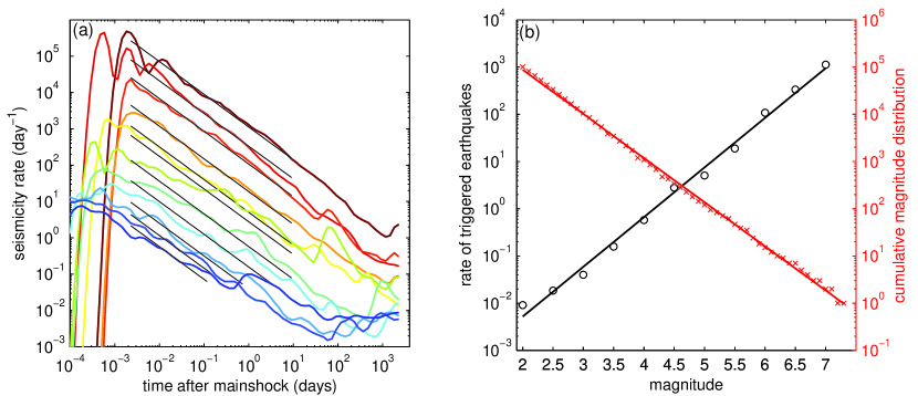
Figure 2: Same as Figure 1 except that we have used $m_{d}=2$ and we have corrected the seismicity rate for missing early aftershocks using (12) (assuming GR law with $b=1$). We fit the seismicity rate in the time interval $0.002<t<10$ days and for $\lambda(t,m_{M})>0.1$ day^-1. The fit of $K(m_{M})$ give $K_{0}=0.0041$ day^p-1 and $\alpha=1.05$.

The results are shown in Fig. 2: the rate of seismicity now follows the Omori law for $t\geq 2\times 10^{-3}$ days for all mainshock magnitudes. The cut-off at $t\approx 10^{-3}$ days (86 sec) is probably due to the fact that earthquakes at such small times cannot be distinguished from the mainshock and are therefore not reported in the catalog.

We have tested different values of the parameters of aftershock and mainshock selection (see Table 1). The fitting interval ($t_{\rm max}$ and $\lambda_{\rm min}$) was adjusted so that the seismicity rate for $t<t_{\rm max}$ and $\lambda(t)>\lambda_{\rm min}$ decays according to Omori’s law with $p\approx 0.9$, as expected for triggered earthquakes. All tests, for reasonable values of $D_{A}$ smaller than the location accuracy (2 km for A-quality locations), give $\alpha=1.05\pm 0.05$. There are however large variations of $K_{0}$ as a function of the parameters of aftershock and mainshock selection. The value of $\alpha$ exceeds the value $\alpha=0.8\pm 0.1$ found by Helmstetter [2003]. This discrepancy is due to differences in the selection of aftershocks and mainshocks. Helmstetter [2003] used a constant value of $R_{F}=50$ km, independent of the “foreshock” magnitude. This value $R_{F}=50$ is too small to exclude distant Landers aftershocks. Helmstetter [2003] also used a larger value of $t_{\rm max}=1$ yr, independent of $m_{M}$, so that a significant fraction of background events may have contaminated aftershocks of small mainshocks.

We have applied the same method (selection of mainshocks and aftershocks, correction for undetected early aftershocks, and fit by Omori’s law) to synthetic catalogs generated with the ETES model. In this model, the seismicity rate $\lambda(t,\vec{r},m)$ is the sum of a constant background term $\mu$ and of aftershocks from all previous earthquakes:

$$\lambda(t,\vec{r},m) = p_{m}(m)\Big{[}\mu+\sum_{t_{i}<t}k10^{\alpha(m-m_{0})}~{}$$ (15)

$$\times{\theta c^{\theta}\over(t+c)^{1+\theta}}~{}{\nu L(m_{i})^{\nu}\over(|\vec{r}-\vec{r_{i}}|+L(m_{i}))^{1+\nu}}\Big{]}\,,$$

where $L(m)=0.01\times 10^{0.5m}$ is the rupture length, $p_{m}(m)$ is the magnitude distribution, $c$, $\theta$, $k$, $\alpha$, $\nu$ are adjustable parameters. Our method recovers the $\alpha$ value of the model with an accuracy $\approx 0.03$, but underestimates the total number of aftershocks, because distant aftershocks outside the “influence zone” used for aftershock selection are missed (see results in Table 1).

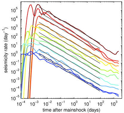
Figure 3: Same as Figure 2 with different parameters $D_{A}=0.5$ km, $N_{L,A}=2$, $D_{F}=3$ km, $N_{L,F}=3$, and without including aftershocks in the influence zone of previous aftershocks.

In order to study the rate of aftershocks at large times after a mainshock, we have selected aftershocks very close to the mainshock, in order to minimize the influence of non-correlated earthquake. We used parameters $D_{A}=0.5$ km, $N_{L,F}=2$, $D_{F}=3$ km, and $N_{L,F}=3$, and we did not include aftershocks in the influence zone of previous aftershocks (see model #8 in Table 1). We thus under-estimate the number of aftershocks for small mainshocks, because the influence zone of small events is smaller than the location accuracy, and because we miss more secondary distant aftershocks for small mainshocks. The results are shown in Figure  3. We observe that the duration of the aftershock sequence is at least 1000 days, independent of the mainshock magnitude, as predicted by the rate-and-state model of seismicity [Dieterich, 1994]. This figure also confirms that Omori’s exponent does not depend on the mainshock magnitude.

The instantaneous increase of seismicity rate after a mainshock, compared to the long-term rate, is at least of a factor $10^{5}$, maybe larger if we could detect aftershocks at shorter times. Using the rate-and-state model [Dieterich, 1994], this means that the ratio $\Delta\sigma/A\sigma_{n}$ (where $\Delta\sigma$ is the maximum Coulomb stress change, $A$ is a parameter of the rate-and-state friction law, and $\sigma_{n}$ is the normal stress) is at least equal to $\log(10^{5})=11.5$. Assuming $A\sigma_{n}=0.4$ bar [Toda and Stein, 2003], this gives a maximum stress of $4.6$ bar.

3.5 Magnitude distribution of triggered earthquakes

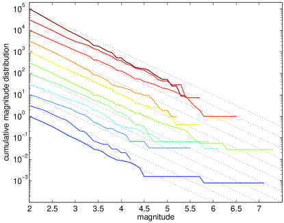
Figure 4: Cumulative magnitude distribution of triggered earthquakes, for mainshock magnitudes ranging from 2 (below) to 7 (top) with a bin size of 0.5. The curves have been normalized by a factor $10^{0.5m_{M}}$ for clarity. Dotted lines represent a GR law with $b=1$ for reference. The number of events decreases with $m_{M}$ (between $N=11502$ for $7\leq m_{M}<7.5$ down to $N=1328$ for $7\leq m_{M}<2.5$) due to the smaller fraction of small earthquakes considered as mainshocks, and due to the shorter time window used for aftershock selection of small mainshocks.

We have analyzed the magnitude distribution of triggered earthquakes for each class of the mainshock magnitude between 2 and 7. As above, we select aftershocks in a time window [$t_{\rm min}(m_{M})$, $t_{\rm max}(m_{M})$] such that the catalog is complete above $m_{d}=2$ and that the influence of non-correlated earthquakes is negligible ($\lambda(t,m_{M})>0.1$ day^-1). The results are shown in Figure 4. We observe that the magnitude distribution of triggered earthquakes follows the GR law with $b\approx 1$, independent of the mainshock magnitude. For $7\leq m_{M}<7.5$ (Hector-Mine and Landers), the $b$-value seems larger than 1. However, if we use $m_{d}=3$ and a smaller minimum time $t_{\rm min}$, the magnitude distribution is close to the GR law with $b=1$. These results imply that a small earthquake can trigger a much larger earthquake. It thus validates our hypothesis that the size of a triggered earthquake is not determined by the size of the trigger, but that any small earthquake can grow into a much larger one [Kagan, 1991b; Helmstetter, 2003; Felzer et al., 2004]. The magnitude of the triggering earthquake controls only the number of triggered quakes.

3.6 Proportion of triggered events in catalogs

We use the scaling of the average number of triggered earthquakes per mainshock and the hypothesis that the magnitude distribution of all quakes follows the GR law to derive the long-term fraction of aftershocks (assuming boundaries in time and space for the definition of aftershocks). The rate of $m\geq m_{d}$ aftershocks triggered, directly or indirectly, by an earthquake of magnitude $m$ at time $t$ after this quake follows approximately

$$\lambda_{m}(t)={K_{0}~{}10^{\alpha m}~{}10^{-bm_{d}}~{}\over t^{p}}\,,$$ (16)

with $p=0.9$ and $K_{0}=0.0041$ day^p-1. This relation holds at least for times $t>0.001$ day (86 sec), for all mainshock magnitudes, after correcting for the incompleteness of the catalog at short times using eq. (12). For $m\geq 7$, the Omori law decay holds at least up to $T\approx 100$ days. If we assume that this “aftershock duration” does not depend on the mainshock magnitude, the average total number of $m>2$ aftershocks (including secondary aftershocks) triggered by $m\geq m_{d}$ mainshocks in the time window $c<t<T$ is

$$N_{\rm aft}(m)=\int\limits_{c}^{T}\lambda_{m}(t)dt=K_{0}~{}10^{\alpha m-bm_{d}}{T^{1-p}-c^{1-p}\over 1-p}\,.$$ (17)

Averaging over all magnitudes of the mainshock we can compute the average total number $N_{\rm aft}$ of $m\geq m_{d}$ aftershocks (including secondary aftershocks) per mainshock of magnitude $m_{d}<m<m_{\rm max}$. Assuming a GR law with $b=1$ and with an upper magnitude cut-off at $m=m_{\rm max}$, $N_{\rm aft}$ is given by

$$N_{\rm aft} = \int\limits_{m_{d}}^{m_{\rm max}}p_{(}m)~{}N_{\rm aft}(m)~{}dm$$

$$= K_{0}~{}{T^{1-p}-c^{1-p}\over 1-p}~{}\int\limits_{m_{d}}^{m_{\rm max}}b~{}\ln(10)~{}10^{-bm}10^{\alpha m}dm$$

$$= {K_{0}b~{}10^{(\alpha-b)m_{d}}\over b-\alpha}\left[1-10^{(\alpha-b)~{}(m_{\rm max}-m_{d})}\right]~{}{T^{1-p}-c^{1-p}\over 1-p}\,.$$

The special case $\alpha=b$ gives

$$N_{\rm aft}=K_{0}b\ln(10)~{}(m_{\rm max}-m_{d})~{}~{}{T^{1-p}-c^{1-p}\over 1-p}\,.$$ (19)

Using the parameters $\alpha=1.05$, $b=1.$, $c=0.001$ day, $K_{0}=0.0041$ day^p-1, and $m_{d}=2$ estimated for Southern California (see Table 1 line 2) and assuming a maximum magnitude $m_{\rm max}=8$ and an aftershock duration $T=100$ days, we obtain $N_{\rm aft}=1.11$. In other words, a fraction $N_{\rm aft}/(N_{\rm aft}+1)=53$% of $m\geq 2$ earthquakes in California are aftershocks of a $m\geq 2$ earthquake. If we assume that Omori’s law with $p=0.9$ holds up to $T=10000$ days (27 yrs), then $N_{\rm aft}=2.06$ (67% of earthquakes are aftershocks). The results do not depend on $c$ if $p<1$. The fraction of aftershocks increases if we include mainshocks with $m\leq 2$. Assuming that equation (17) and the GR law still hold down to $m_{d}=-1$ [Abercrombie, 1995], we obtain $N_{\rm aft}=2$ for $T=100$ days: 67% of earthquakes of any magnitude are triggered by earthquakes of magnitude $m\geq-1$. The fraction of triggered events goes to 1 as the minimum magnitude $m_{d}$ goes to $-\infty$ [Sornette and Werner, 2004].

Our results are relatively close to the generic model of Californian aftershocks Reasenberg and Jones [1989, 1994] (RJ), which assumed

$$\lambda_{m}(t)={10^{a+b(m-m_{d})}\over(t+c)^{p}}\,,$$ (20)

with $c=0.05$ days, $p=1.08$, $b=0.91$, $a=-1.67$ [Reasenberg and Jones, 1994]. Their model gives $K_{0}=10^{a}=0.017$ day^-1 for $m_{d}=2$, but with smaller $\alpha$ and $b$ values ($\alpha$ is assumed to be equal to $b$), so that the rate of $m\geq 2$ aftershocks at $t=1$ day and for $m=7$ is $\lambda_{m}(t)=758$ day^-1 for RJ model and $\lambda_{m}(t)=729$ day^-1 for our model (line #2 in Table 1).

4 Scaling of stress transfers with the mainshock magnitude

Computing stress changes induced by a small earthquake at the location of another quake is very difficult. The stress field created by an earthquake is sensitive to the slip distribution on the fault, at least for small distances from the fault plane [Steacy et al., 2004]. Slip distribution is usually available only for large $m\geq 6$ earthquakes in California. For small earthquakes, we can use a point-source model if we know the focal mechanism, to calculate stress for distances from the fault much larger than the rupture dimension. We can also estimate the most likely focal plane from the fault orientations in the area or from the orientation of the tectonic stress. Then we can model the rupture by a rectangular dislocation with a uniform or tapered slip. But this simple source model would still be incorrect close to the fault, where most aftershocks are located.

Marsan [2004] solved this problem by computing the distribution of the stress induced by an earthquake at the location of another earthquake, and by studying only the tail of the distribution (small absolute value of stress) corresponding to distances larger than the rupture length of the event. Marsan [2004] concluded that small earthquakes are at least as important as larger ones for redistributing stress between events. This result is in agreement with our result for scaling the number of triggered earthquakes with the mainshock magnitude. But even in the far field, these calculations of the Coulomb stress change induced by an earthquake are very inaccurate, because the accuracy of focal mechanisms is on the order of 30^∘ [Kagan, 2002b]. Another problem in [Marsan, 2004] is that he considers earthquakes of magnitude $m=3$, which have a rupture length $L\approx 300$ m, much smaller than the average accuracy on vertical coordinates of 4 km. These location errors can significantly bias any estimate of the stress change induced by small $m<5$ quakes [Huc and Main, 2003].

The observation that earthquake triggering scales with the magnitude $m$ of the trigger as $\sim 10^{\alpha m}$ with $\alpha\approx b$ suggests that small events should not be neglected in studying stress interactions between quakes. However, directly calculating the stress induced by a small events is impossible due to the inaccuracy of earthquake locations and focal mechanisms. Even if we cannot compute the spatial distribution of the stress induced by a small earthquake, we can estimate how such small events trigger others. On average the total number of events triggered by an earthquake (integrated over space) will be independent of the earthquake source. For instance, we can account for the influence of small earthquakes in the rate-and-state model of Dieterich [1994] by using for such small events a point source model which, as we know, depends only on the focal mechanism. We can then compute the seismicity rate on each point of a grid by integrating on each cell that rate estimated using equation (12) of [Dieterich, 1994] (using space-variable stress for a point-source model). If the size of each cell is equal to a few km, a point source model approximates $m\leq 4$ earthquakes well, because the integral of the seismicity rate over each cell depends only slightly on the geometry of the rupture fault and the variations of fault slip.

Another alternative is to use empirical laws like the ETES model [Kagan and Knopoff, 1987b; Felzer et al., 2003a; Helmstetter et al., 2004], rather than stress calculations and physical models of stress interactions. We can estimate the spatial distribution of future aftershocks for a large earthquake by smoothing the locations of early aftershocks. A magnitude $m=7$ quake has enough aftershocks in the first hour to estimate the distribution of future aftershocks [Helmstetter et al., 2004]. In contrast, predictions based on Coulomb stress change calculations require a good model of slip distribution on the fault, which is not available until a few hours after the mainshock at best.

5 Spatial distribution of seismicity

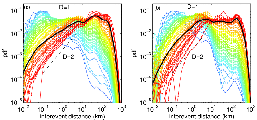
Figure 5: Distribution of distances between hypocenters $p_{r}(r,t)$ for SHLK (a) and HCS (b) catalogs, using only earthquake pairs with inter-event times in the range [$t$, $1.25t$], where $t$ increases between 1.4 minutes (blue curve) to 2500 days (red curve). The fractal dimension of $p_{r}(r)$, measured for $0.1\leq r\leq 5$ km for all earthquakes (black lines), is $D=1.54$ for SHLK catalog and $D=1.73$ for HCS catalog.

We have estimated the distribution of distances between hypocenters $p_{r}(r)$, using the relocated catalogs for Southern California by Hauksson et al. [2003] (HCS) and Shearer et al. [2003] (SHLK). These catalogs apply waveform cross-correlation to obtain precise differential times between nearby events. These times can then be used to greatly improve the relative location accuracy within clusters of similar events. Locations in these two catalogs do not always agree in detail, reflecting their different modeling assumptions and seismic velocity structures. However, their overall agreement is quite good, particularly when compared to the standard catalog locations. In many regions, these new catalogs resolve individual faults in what previously appeared to be diffuse earthquake clouds. In both catalogs, we have selected only $m\geq 2$ earthquakes relocated with an accuracy of $\epsilon_{h}$ and $\epsilon_{z}$ smaller than 100m. In the HCS catalog, there are 71943 $m\geq 2$ earthquakes between 1984 and 2002, out of which 24127 (34%) are relocated with $\epsilon_{h}<0.1$ km and $\epsilon_{z}<0.1$ km. In the SHLK catalog, there are 82442 $m\geq 2$ earthquakes in the same period [1984, 2002], out of which 33676 (41%) are relocated with $\epsilon_{h}<0.1$ km and $\epsilon_{z}<0.1$ km. The probability density function of distances $p_{r}(r)$ between hypocenters is close to a power-law $p_{r}(r\sim r^{D-1}$ in the range $0.1\leq r\leq 5$ km. The correlation fractal dimension (measured by least-square linear regression of $\log(r)$ and $\log(p_{r}(r))$ for $0.1\leq r\leq 5$ km) is $D=1.54$ for SHLK and $D=1.73$ for HCS (see black lines in Figure 5). The faster decay for $r<0.1$ km is due to location errors, and the roll-off for distances $r>5$ km is due to the finite thickness of the seismogenic crust. The difference in the $D$-value between the two catalogs may come from larger location errors in HCS, but also from errors in estimating the $D$-value (see Kagan [2004c] for a discussion of errors and biases in determining the fractal correlation dimension).

To check the accuracy of the $D$-value, we tested a synthetic catalog, generated with the same number of events as the real catalog. We used random longitudes and latitudes, with a uniform epicentral distribution within the same boundaries as real data. Depths in the synthetic catalog were chosen by shuffling the depths of earthquakes from the real catalog to keep the same depth distribution. The fractal dimension in the range $0.1\leq r\leq 5$ km was $D=2.93\pm 0.04$: a little smaller than the value $D=3$ expected for a purely uniform distribution in a volume. This discrepancy is due to three factors: the finite number of events, the non-uniform distribution of depths, and finite size effects.

The spatial clustering of earthquake hypocenters measured for the full catalog is due both to the fault network structure and to earthquake interactions. The latter modify long-term spatial distribution by increasing the fraction of small inter-event distances, that is decreasing the fractal dimension [Kagan, 1991a]. The clustering of aftershocks around mainshocks, and of secondary aftershocks close to the direct aftershock of the mainshocks, and so on, can create a fractal distribution. This results from the scaling of the aftershock zone with magnitude coupled with the GR law, without any underlying fractal fault structure [Helmstetter and Sornette, 2002].

Over very long time intervals, triggered earthquakes should be located uniformly on the fault network, and the fractal dimension of the whole catalog should reach a constant value. In our model described in equation (5), $p_{r}(r)$ represents the “long-term” time-independent spatial distribution of seismicity. Distribution $p_{r}(r)$ gives the average density of earthquakes at a distance $r$ from the mainshock due to fault structure geometry and the fault s time-independent heterogeneity. This does not take into account earthquake interactions. The effect of the mainshock, which increases or decreases the seismicity rate at close distances by modifying the stress, is described in the factor $f(\sigma,t)$ in (5). Therefore, we should not use in (5) the function $p_{r}(r)$ estimated from the catalogs of Southern California seismicity because these catalogs cover less than 20 years and contain a majority of aftershocks. If we had included that function, we would be double-counting earthquake interactions.

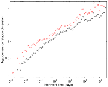
Figure 6: Fractal dimension of $p_{r}(r,t)$ as a function of inter-event time $t$, using SHLK catalog (diamonds) and HCS catalog (circles).

To estimate and remove the time dependence of the spatial distribution of inter-event distances, we have measured that distribution $p_{r}(r,t)$ using only earthquake pairs with an inter-event time $\tau$ in the range [$t$, $t+dt$]. The results are shown in Figure 5. As the minimum inter-event time increases, the fraction of small distances will decrease. The fractal dimension of $p_{r}(r,t)$ increases between $D\approx 0$ at times $t=5$ minutes up to $D\approx 2$ for $t=2500$ days (see Figure 6). This maximum inter-event time of 2500 days is long enough so that earthquake interactions are negligible compared to tectonic loading, and a very small fraction of earthquake pairs with $\tau>1000$ days belong to the same aftershock sequence. This value $D=2$, measured for $t=2500$ days, can thus be interpreted as the fractal dimension of the active fault network.

6 Conclusion

Although large earthquakes are much more important than smaller ones for energy release, small quakes have collectively the same influence as large ones for stress changes between earthquakes, due to seismic spatial clustering. Because the stress drop is constant, the stress change induced by an earthquake of magnitude $m$ at the location of other earthquakes (located on a fractal network of dimension $D$) increases with $m$ as $\sim 10^{Dm/2}$. Measuring directly the scaling of such stress change with magnitude is difficult, because the accuracy of earthquake locations and focal mechanisms is limited. We can, however, estimate indirectly the relative importance of small and large events for stress transfer by studying the properties of triggered seismicity. If quakes are triggered by static stress changes, then the number of such triggered events should also scale as $\sim 10^{Dm/2}$ with the magnitude of the trigger.

We have measured the average seismic rate triggered by an earthquake for Southern California seismicity. We found that the rate of triggered events decays with time according to Omori’s law $\sim 1/(t+c)^{p}$ with $p=0.9$ and $c<3$ minutes (after correcting for the increase in the completeness threshold after a large mainshock, see eq. 12). This decay is independent of the mainshock magnitude $m$ for $2<m<7.5$. We also found that the magnitude of triggered aftershocks follows the Gutenberg-Richter law with $b=1$ and is independent of the mainshock magnitude. The rate of triggered quakes increases with $m$ as $\sim 10^{\alpha m}$, with an exponent $\alpha=1.05\pm 0.05$.

We have measured the fractal correlation dimension $D$ for two different catalogs of relocated earthquakes in Southern California, given by the exponent of the cumulative distribution of the distances between all pairs of hypocenters. This fractal dimension $D\approx 1.6$, measured in a limited time-window, characterizes the spatial clustering of earthquakes due to fault network structure and earthquake interactions. By using only earthquake pairs with inter-event times larger than a threshold to compute $D$, we have tried separating the effects that fault geometry and earthquake triggering have upon spatial clustering. For inter-event times larger than 1000 days, we obtain $D\approx 2$. Thus, our result $\alpha\approx D/2$ supports the assumption that earthquakes are triggered by static stress from past events.

The fact that $\alpha$ is nearly equal to the $b$-value has important consequences for earthquake triggering. It means that equal magnitude bands contribute equally to stress at the location of a future hypocenter, e.g., earthquakes with $2<m<5$ have collectively the same importance as $5<m<8$ events for stress changes and for triggering, because the frequency of small earthquakes compensates for their lower triggering potential. Even if explicit stress calculations based on cataloged earthquakes have limited accuracy, we can estimate how small earthquakes affect earthquake triggering. This can be done with a spatial resolution of a few km, using an ETES model or the more physical rate-and-state model.

Table 1: Scaling of aftershock productivity and earthquake frequency with magnitude. Times are in days and distances in km. Parameters $\Delta m$, $D_{F}$, $D_{A}$, $N_{L,F}$, $N_{L,A}$ and $T_{F}$ are used in the selection of mainshocks and aftershocks (see section 3.3). Parameters $t_{\rm min}$, $t_{\rm max}$ and $\lambda_{\rm min}$ define the time interval used to estimate the scaling of the number of aftershocks with the mainshock magnitude (see section 3.4). $N$ is the total number of events with $m\geq m_{d}$ and $N_{ms}$ is the number of mainshocks. $K_{0}$ defined by (13) measures aftershock productivity.

#	$m_{d}$	time	$\Delta m$	$D_{F}$	$D_{A}$	$N_{L,F}$	$N_{L,A}$	$T_{F}$	$t_{\rm min}$	$t_{\rm max}$	$\lambda_{\rm min}$	$\alpha$	$N$	$N_{ms}$	$K_{0}$
1	2	1980-2004	1	3	2	3	2	365	0.0020	10	0.100	0.99	101402	19247	0.0092
2c	2	1980-2004	1	3	2	3	2	365	0.0020	10	0.100	1.05	101402	19247	0.0041
3c	2	1980-2004	1	3	2	3	2	36	0.0020	10	0.100	1.02	101402	33123	0.0065
4c	2	1980-2004	1	3	2	3	2	730	0.0020	10	0.100	1.06	945736	15130	0.0035
5c	2	1980-2004	0	3	2	3	2	365	0.0020	10	0.100	0.95	101402	26004	0.0167
6c	2	1980-2004	2	3	2	3	2	365	0.0020	10	0.100	1.09	101402	18784	0.0024
7c	2	1980-2004	1	3	3	3	3	365	0.0020	10	0.500	1.04	101402	19247	0.0048
8a,c	2	1980-2004	1	3	0.5	3	2	365	0.0020	10	0.005	1.16	101402	19247	0.0009
9a,c	2	1980-2004	1	3	0.5	3	2	365	0.0020	100	0.000	1.15	101402	19247	0.001
10a,c	2	1980-2004	1	3	0.5	3	2	365	0.0020	1000	0.000	1.12	101402	19247	0.0013
11c	2	1980-2004	1	1	4	1	4	365	0.0020	10	5.000	0.94	101402	37839	0.0193
12c	2	1980-2004	1	1	2	1	2	365	0.0020	10	2.000	1.01	98805	36864	0.0078
13c	2	1980-2004	1	4	1	4	1	365	0.0020	10	0.100	1.13	101402	15153	0.001
14c	2	1980-2004	1	4	4	4	4	365	0.0020	10	0.100	1.02	101402	15153	0.0064
15c	2	1980-2004	1	1	1	1	1	365	0.0020	10	0.500	1.05	101402	37839	0.003
16c	2	1980-1992.4	1	3	2	3	2	365	0.0020	10	0.100	1.00	40565	9603	0.0056
17c	2	1992.4-2004	1	3	2	3	2	365	0.0020	10	0.100	1.05	60837	9187	0.0041
18	3	1980-2004	1	3	2	3	2	365	0.0003	10	0.010	1.07	101402	19247	0.0033
19c	3	1980-2004	1	3	2	3	2	365	0.0020	10	0.010	1.10	101402	19247	0.0023
20b,c	2	1980-2004	1	3	3	4	2	36	0.0020	10	0.500	1.01	101402	29210	0.0075
21c	2	1980-2004	1	3	3	4	2	36	0.0020	10	0.500	1.02	101402	32801	0.006