Canonical Lie-transform method in Hamiltonian gyrokinetics: a new approach

Abstract

The well-known gyrokinetic problem regards the perturbative expansion related to the dynamics of a charged particle subject to fast gyration motion due to the presence of a strong magnetic field. Although a variety of approaches have been formulated in the past to this well known problem, surprisingly a purely canonical approach based on Lie transform methods is still missing. This paper aims to fill in this gap and provide at the same time new insight in Lie-transform approaches.

1 Introduction: transformation approach to gyrokinetic theory

A great interest for the description of plasmas is still vivid in the scientific community. Plasmas enter problems related to several fields from astrophysics to fusion theory. A crucial and for some aspects still open theoretical problem is the gyrokinetic theory, which concerns the description of the dynamics for a charged point particle immersed in a suitably intense magnetic field. In particular, the “gyrokinetic problem” deals with the construction of appropriate perturbation theories for the particle equations of motion, subject to a variety of possible physical conditions. Historically, after initial pioneering work Alfen 1950 ; Gardner 1959 ; Northrop et al. 1960 , and a variety of different perturbative schemes, a general formulation of gyrokinetic theory valid from a modern perspective is probably due to Littlejohn Littlejohn1979 , based on Lie transform perturbation methods Littlejohn1981 ; Littlejohn1982 ; Littlejohn1983 ; Cary et al. 1983 . For the sake of clarity these gyrokinetic approaches can be conveniently classified as follows (see also Fig.1):
A) direct non-canonical transformation methods: in which non-canonical gyrokinetic variables are constructed by means of suitable one-step Alfen 1950 , or iterative, transformation schemes, such as a suitable averaging technique Morozov 1966 , a one-step gyrokinetic transformation Bernstein , a non-canonical iterative scheme Balescu 1986 . These methods are typically difficult (or even impossible) to be implemented at higher orders;
B) canonical transformation method based on mixed-variable generating functions: this method, based on canonical perturbation theory, was first introduced by Gardner Gardner 1959 ; Gardner et al. 1959 and later used by other authors Weitzner 1995 ). This method requires, preliminarily, to represent the Hamiltonian in terms of suitable field-related canonical coordinates, i.e., coordinates depending on the the topology of the magnetic flux lines. This feature, added to the unsystematic character of canonical perturbation theory, makes its application to gyrokinetic theory difficult, a feature that becomes even more critical for higher-order perturbative calculations;
C) non-canonical Lie-transform methods: these are based on the adoption of the non-canonical Lie-transform perturbative approach developed by Littlejohn Littlejohn1979 . The method is based on the use arbitrary non-canonical variables, which can be field-independent. This feature makes the application of the method very efficient and, due to the peculiar features for the perturbative scheme, it permits the systematic evaluation of higher-order perturbative terms. The method has been applied since to gyrokinetic theory by several authors Dubin1983 ; Lee1983 ; Hahm 1988 ; Brizard 1995 ;
D) canonical Lie-transform methods applied to non-canonical variables: see for example Hahm Lee Brizard 1988 . Up to now this method has been adopted in gyrokinetic theory only using preliminar non-canonical variables, i.e., representing the Hamiltonian function in terms of suitable, non-canonical variables (similar to those adopted by Littlejohn). This method, although conceptually similar to the developed by Littlejohn, is more difficult to implement.

All of these methods share some common features,in particular:
- they may require the application of multiple transformations, in order to construct the gyrokinetic variables;
- the application of perturbation methods requires typically the representation of the particle state in terms of suitable, generally non-canonical, state variables. This task may be, by itself, difficult since it may require the adoption of a preliminary perturbative expansion.
An additional important issue is the construction of gyrokinetic canonical variables. The possibility of constructing canonical gyrokinetic variables has relied, up to now, on essentially two methods, i.e., either by adopting a purely canonical approach, like the one developed by Gardner Gardner 1959 ; Gardner et al. 1959 , or using the so-called “Darboux reduction algorithm”, based on Darboux theorem Littlejohn1979 . The latter is obtained by a suitable combination of dynamical gauge and coordinate transformations, permitting the representation of the fundamental gyrokinetic canonical 1-form in terms of the canonical variables. The application of both methods is nontrivial, especially for higher order pertubative calculations. The second method, in particular, results inconvenient since it may require an additional perturbative sub-expansion for the explicit evaluation of gyrokinetic canonical variables.
For these reasons a direct approach to gyrokinetic theory, based on the use of purely canonical variables and transformations may result a viable alternative. Purpose of this work is to formulate a “purely” canonical Lie-transform theory and to explicitly evaluate the canonical Lie-generating function providing the canonical gyrokinetic transformation.

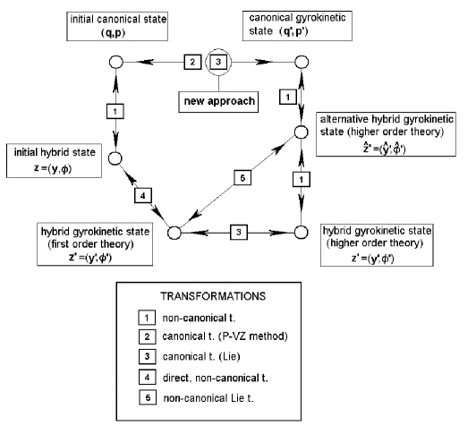
Figure 1: The transformation approach to gyrokinetic theory: 2: see GardnerGardner 1959 ,Gardner et al. 1959 ; 3: see Hahm et al. Hahm Lee Brizard 1988 and present theory; 4: first obtained by Alfven Alfen 1950 ; 5: see Littlejohn Littlejohn1979 .

2 Lie-trasform perturbation theory

We review some basic aspects of perturbation theory for classical dynamical systems. Let us consider the state $\mathbf{x}$ of a dynamical system and its $d$-dimensional phase-space $M$ endowed with a vector field $X$. With respect to some variables $\mathbf{x}=\left\{x^{i}\right\}$ we assume that $\mathbf{X}$ has representation Littlejohn1982

$$\frac{dx^{i}}{dt}=X^{i}$$ (1)

where ${\epsilon}$ is an ordering parameter. We treat all power series formally; convergence is of secondary concern to us. By hypothesis, the leading term $\mathbf{X}_{0}$ of (1) represents a solvable system, so that the integral curves of $\mathbf{X}$ are approximated by the known integral curves of $\mathbf{X}_{0}$. The strategy of perturbation theory is to seek a coordinate transformation to a new set of variables $\left\{\bar{x}^{i}\right\}$, such that with respect to them the new equations of motion are simplified. Since (1) is solvable at the lowest order, the coordinate transformation is the identity at lowest order, namely

$$\bar{x}^{i}=x^{i}+O({\epsilon})$$ (2)

The transformation is canonical if it preserves the fundamental Poisson brackets. It can be determined by means of generating functions, Lie generating function or mixed-variables generating functions, depending on the case. In the Lie transform method, one uses transformations $T$ which are represented as exponentials of some vector field, or rather compositions of such transformations. To begin, let us consider a vector field $G$, which is associated with the system of ordinary differential equations

$$\frac{dx^{i}}{d{\epsilon}}=G^{i}(x),$$ (3)

so that if $x$ and $\bar{x}$ are initial and final points along an integral curve (3), separated by an elapsed parameter ${\epsilon}$, then $\bar{x}=Tx$. In the usual exponential representation for advance maps, we have

$$T=\exp({\epsilon}G).$$ (4)

We will call $G$ the generator of the transformation $T$. In Hamiltonian perturbation theory the transformation $T$ is usually required to be a canonical transformation. Canonical transformations have the virtue that they preserve the form of Hamilton’s equations of motion. Canonical transformation can be represented by mixed-variable generating function, as in the Poincare-Von Zeipel method or by means of Lie transform. In the latter method vector fields $G$ are specified through the Hamilton’s equations. Following a more conventional approach, we can write the (3) in terms of the transformed point

$$\frac{d\bar{\mathbf{x}}}{d{\epsilon}}=\left[\bar{\mathbf{x}},\omega\right]$$ (5)

The components of the above relation are just Hamilton’s equations in Poisson bracket notation applied to the “Hamiltonian” (Lie generating function) $\omega$, with the parameter ${\epsilon}$ the “time.” Equation (5) therefore generates a canonical transformation for any ${\epsilon}$ to a final state $\mathbf{\bar{x}}$ whose components satisfy the Poisson bracket condition

$$\left[\bar{q}_{i},\bar{q}_{j}\right]=\left[\bar{p}_{i},\bar{p}_{j}\right]=0$$ (6)

$$\left[\bar{q}_{i},\bar{p}_{j}\right]=\delta_{ij}.$$ (7)

To find the transformation $T$ explicitly, we introduce the Lie operator $L=\left[\omega,\dots\right]$. Recalling that coordinate components of vector are subject to pull back transformation law, then one gets

$$\frac{dT}{d{\epsilon}}=-TL$$ (8)

with the formal solution

$$T=\exp\left[-\int^{{\epsilon}}L\left({\epsilon}^{\prime}\right)d{{\epsilon}}^{\prime}\right].$$ (9)

For any canonical transformation the new Hamiltonian $\bar{H}$ is related to the old one by

$$\bar{H}=T^{-1}H+T^{-1}\int^{\epsilon}_{0}d{\epsilon}^{\prime}T\left({\epsilon}^{\prime}\right)\frac{\partial\omega\left({\epsilon}^{\prime}\right)}{\partial t}.$$ (10)

To obtain the perturbation series one can expand $\omega,L,T,H$ and $\bar{H}$ as power series in ${\epsilon}$

$$M=\sum_{n=0}^{\infty}{\epsilon}^{n}M_{n}$$ (11)

where $M$ represents $\omega,L,T,H$. From (8), equating like powers of ${\epsilon}$, we obtain a recursion relation for the $\omega_{n},L_{n},T_{n},H_{n}\ \ (n>0)$ which with $T_{0}=1$, gives $T_{n}$ in terms of $L_{n}$ and $\omega_{n}$ in all orders.

3 The canonical Lie transform approach to gyrokinetic theory

The customary approach based on Lie-transform methods and due to Littlejohn Littlejohn1979 adopts “hybrid” (i.e., non-canonical and non-Lagrangian) variables to represent particle state, i.e., of the form $\mathbf{z=(y,}\phi\mathbf{)}$. There are several reasons, usually invoked for this choice. In the first place, the adoption of hybrid variables may be viewed, by some authors, as convenient for mathematical simplicity. However, the subsequent calculation of canonical variables (realized by means of Darboux theorem) may be awkward and give rise to ambiguities issues Weitzner 1995 . Other reasons may be related to the the ordering scheme to adopted in a canonical formulation: in fact, in gyrokinetic theory, the vector potential $\mathbf{A}$ in the canonical momentum must be regarded of order $1/O(\varepsilon)$ while keeping the linear momentum of zero order, i.e., $\mathbf{p=}m\mathbf{v+}\frac{q}{\varepsilon c}\mathbf{A.}$ As a consequence, in a perturbative theory $\mathbf{p}$ must be expanded retaining at the same time terms of order $1/O(\varepsilon)$ and $O(\varepsilon^{0})$, a feature which may give rise to potential ambiguities.  According to Littlejohn Littlejohn1979 this can be avoided by the adoption of suitable hybrid variables, which should permit to decouple at any order the calculations of the perturbations determined by means of suitable Lie-generators. However, a careful observation reveals that the same ambiguity (ordering mixing) is present also in his method. In fact, one finds that the first application of the non-canonical Lie-operator method, yielding the lowest order approximation for the variational fundamental 1-form, provides non-trivial contributions carried by the first order Lie-generators. Probably for this reason, his approach is usually adopted only for higher-order calculations where ordering mixing does not appear.

In this paper we intend to point out that canonical gyrokinetic variables can be constructed, without ambiguities, directly in terms a a suitable canonical Lie-transform approach, by appropriate selection of the initial and final canonical states (see path

$$\mathbf{x}\rightarrow\mathbf{X}^{\prime}=\mathbf{x+\varepsilon}\left[\mathbf{X}^{\prime},\omega\right],$$ (12)

being $\omega=\omega(\mathbf{X}^{\prime},\varepsilon)$ the corresponding Lie generator. In order to achieve this result, we shall start demanding the following relation between the fundamental differential 1-forms, i.e., the initial and the gyrokinetic Lagrangians, which can be shown to be of the form:

$$dt\emph{L}(\mathbf{x},\frac{d}{dt}\mathbf{x,}t)=dt\mathcal{L}(\mathbf{X}^{\prime},\frac{d}{dt}\mathbf{X}^{\prime}\mathbf{,}t)+dS_{1}+dS_{2}+dS_{3}+dS_{4}.$$ (13)

Here $S_{1},S_{2},S_{3},S_{4}$ are suitable dynamical gauges functions, i.e.,

$$S_{1}=\varepsilon\left(\mathbf{\rho}^{\prime}\mathbf{\cdot}\frac{Ze}{\varepsilon c}\mathbf{A}^{\prime}\right),$$ (14)

$$S_{2}=\frac{1}{2}\frac{Ze}{c}\mathbf{\rho}^{\prime}\cdot\nabla^{\prime}\mathbf{A}^{\prime}\cdot\mathbf{\rho}^{\prime},$$ (15)

$$S_{3}=\varepsilon\mathbf{\rho}^{\prime}\cdot m\mathbf{v,}$$ (16)

$$S_{4}=m\int dQ^{\prime}v_{Q}(\psi_{p}^{\prime},Q^{\prime},Q_{1}^{\prime},t),$$ (17)

where $m$ and $Ze$ are respectively the mass, the electric charge of the particle and $\varepsilon\mathbf{\rho}^{\prime}=-\varepsilon\frac{\mathbf{w}^{\prime}\mathbf{\times b}^{\prime}}{\Omega^{\prime}}$ the Larmor radius. Moreover, $\mathbf{w}^{\prime}$ is a vector in the plane orthogonal to the magnetic flux line, while $\mathbf{b}^{\prime}=\mathbf{B}(\mathbf{r}^{\prime},t)/B(\mathbf{r}^{\prime},t),$ $\Omega^{\prime}=\frac{ZeB^{\prime}}{mc}$is the Larmor frequency and finally primes denote quantities evaluated at the guiding center position $\mathbf{r}^{\prime}$. In particular, $v_{Q}\equiv v_{Q}(\psi_{p}^{\prime},Q^{\prime},Q_{1}^{\prime},t)$ To the leading order in $\varepsilon$ one can prove

$$\mathbf{r} = \mathbf{r}^{\prime}+\varepsilon\mathbf{\rho}^{\prime},$$ (18)

$$\mathbf{v} = \mathbf{v}^{\prime}+\mathbf{w}^{\prime}\mathbf{.}$$ (19)

The remaining notation is standard. Thus, up to $O(\varepsilon)$ terms, there results

$$\left\{\begin{array}[]{c}\mathbf{v}^{\prime}=u^{\prime}\mathbf{b}^{\prime}+\mathbf{v}_{E}^{\prime},\\ \mathbf{w}^{\prime}\mathbf{=}w^{\prime}\left(\mathbf{e}_{1}^{\prime}\cos\phi^{\prime}+\mathbf{e}_{2}^{\prime}\sin\phi^{\prime}\right),\\ \phi^{\prime}=arctg\left\{\frac{\left(\mathbf{v-v}_{E}^{\prime}\right)\cdot\mathbf{e}_{2}^{\prime}}{\left(\mathbf{v-v}_{E}^{\prime}\right)\cdot\mathbf{e}_{1}^{\prime}}\right\},\\ w^{\prime}\equiv\sqrt{2B^{\prime}\mu^{\prime}},\\ P_{\phi}^{\prime}\ =-\frac{mc}{Ze}\mu^{\prime},\end{array}\right.$$ (20)

where $\mathbf{v}_{E}^{\prime}=c\mathbf{E}^{\prime}\times\mathbf{b}^{\prime}/B^{\prime}$ is the electric drift velocity and evaluated at the guiding center position and $\mu^{\prime}$ is the magnetic moment, both evaluated at the guiding center position. Here we have adopted the representation of the magnetic field by means of the curvilinear coordinates $(\psi_{p}{}^{\prime},Q^{\prime},Q^{\prime}_{1})$ where $\psi_{p}{}^{\prime},Q^{\prime}$ are the Clebsch potentials according to which the magnetic field reads $\mathbf{B}^{\prime}=\nabla\psi_{p}^{\prime}\times\nabla Q^{\prime}$, whereas we have introduced the covariant representation for the electric drift velocity $\mathbf{v}_{E}^{\prime}=v_{\psi_{p}}^{\prime}\nabla\psi_{p}^{\prime}+v_{Q}^{\prime}\nabla Q^{\prime}$. The gyrokinetic Hamiltonian $\mathcal{K}(\mathbf{x}^{\prime},t)$, defined by means of

$$\mathcal{K}(\mathbf{X}^{\prime},t)=P_{Q_{1}}^{\prime}\frac{dQ_{1}^{\prime}}{dt}+P_{\psi_{p}}^{\prime}\frac{d\psi_{p}^{\prime}}{dt}+P_{\phi}^{\prime}\frac{d\phi^{\prime}}{dt}-\mathcal{L}(\mathbf{X}^{\prime},\frac{d}{dt}\mathbf{X}^{\prime}\mathbf{,}t)$$ (21)

reads

$$\mathcal{K}(\mathbf{X}^{\prime},t)=-\Omega^{\prime}P_{\phi}^{\prime}+\mathcal{T}+\frac{Ze}{\varepsilon}\Phi^{{}^{\prime}}+$$

$$+\left(P_{Q_{1}}^{\prime}+m\frac{\partial}{\partial Q_{1}^{\prime}}\left(\int dQ^{\prime}v_{Q}^{\prime}\right)\right)\frac{\partial}{\partial t}Q_{1}^{\prime}+\left[P_{\psi_{p}}^{\prime}+m\frac{\partial}{\partial\psi_{p}^{\prime}}\left(\int dQ^{\prime}v_{Q}^{\prime}\right)\right]\frac{\partial}{\partial t}\psi_{p}^{\prime}+m_{s}v_{Q}^{\prime}\frac{\partial}{\partial t}Q^{\prime}.$$ (22)

Here $\mathcal{T}$ is the kinetic energy term, whereas canonical momenta read

$$P_{Q_{1}}^{\prime}=\frac{\partial}{\partial\overset{\cdot}{Q_{1}^{\prime}}}\mathcal{L}(\mathbf{X}^{\prime},\frac{d}{dt}\mathbf{X}^{\prime}\mathbf{,}t)=\frac{\partial}{\partial\overset{\cdot}{Q_{1}^{\prime}}}\left\{\emph{L}(\mathbf{x},\frac{d}{dt}\mathbf{x,}t)-\frac{dS_{1}}{dt}-\frac{dS_{2}}{dt}-\frac{dS_{3}}{dt}-\frac{dS_{4}}{dt}\right\},$$ (23)

$$P_{\psi_{p}}^{\prime}=\frac{\partial}{\partial\overset{\cdot}{\psi_{p}^{\prime}}}\mathcal{L}(\mathbf{X}^{\prime},\frac{d}{dt}\mathbf{X}^{\prime}\mathbf{,}t)=\frac{\partial}{\partial\overset{\cdot}{\psi_{p}^{\prime}}}\left\{\emph{L}(\mathbf{x},\frac{d}{dt}\mathbf{x,}t)-\frac{dS_{1}}{dt}-\frac{dS_{2}}{dt}-\frac{dS_{3}}{dt}-\frac{dS_{4}}{dt}\right\},$$ (24)

$$P_{\phi}^{\prime}=\frac{\partial}{\partial\overset{\cdot}{\phi^{\prime}}}\mathcal{L}(\mathbf{X}^{\prime},\frac{d}{dt}\mathbf{X}^{\prime}\mathbf{,}t)=\frac{\partial}{\partial\overset{\cdot}{\phi^{\prime}}}\left\{\emph{L}(\mathbf{x},\frac{d}{dt}\mathbf{x,}t)-\frac{dS_{1}}{dt}-\frac{dS_{2}}{dt}-\frac{dS_{3}}{dt}-\frac{dS_{4}}{dt}\right\}.$$ (25)

Let us consider, for instance, the equation for $P_{\phi}^{\prime}.$ We notice that $\mathbf{\rho}^{\prime}$ coincides with $\mathbf{g}_{\mathbf{r}^{\prime}}^{(1)}$ the first order Lie generator of the transformation (18). Therefore, $P_{\phi}^{\prime}$ results:

$$P_{\phi}^{\prime}=-\frac{\mathbf{w}}{\Omega}\cdot p_{\mathbf{r}}+\frac{\mathbf{w}^{\prime}}{\Omega^{\prime}}\cdot\left\{\frac{Ze}{c}\mathbf{A}^{\prime}+\frac{1}{2}\frac{Ze}{c}\nabla^{\prime}\mathbf{A}^{\prime}\cdot\mathbf{g}_{\mathbf{r}^{\prime}}^{(1)}+\frac{1}{2}\frac{Ze}{c}\mathbf{g}_{\mathbf{r}^{\prime}}^{(1)}\cdot\nabla^{\prime}\mathbf{A}^{\prime}+m\mathbf{v}\right\}-m\Omega^{\prime}\mathbf{g}_{\mathbf{r}^{\prime}}^{(1)}\cdot\mathbf{g}_{\mathbf{r}^{\prime}}^{(1)}=-\frac{1}{2}m\Omega^{\prime}\mathbf{g}_{\mathbf{r}^{\prime}}^{(1)}\cdot\mathbf{g}_{\mathbf{r}^{\prime}}^{(1)},$$ (26)

where, neglecting contributions of higher orders, the first term on the r.h.s. has been evaluated at the effective position ${\bf r}$. Thus, denoting $P_{\phi}\equiv\frac{\partial\dot{{\bf r}}}{\partial\dot{\phi}}\cdot\frac{\partial}{\partial\dot{{\bf r}}}L({\bf x},\frac{d}{dt}{\bf x},t)=-\frac{\mathbf{w}}{\Omega}\cdot p_{\mathbf{r}}$, the equation can be cast in the following form

$$P_{\phi}^{\prime}\cong P_{\phi}+\varepsilon\left[P_{\phi}^{\prime},\omega\right],$$ (27)

where $\omega$  is the phase function:

$$\omega=m\int dQ^{\prime}v_{Q}(\psi_{p}^{\prime},Q^{\prime},Q_{1}^{\prime},t)+\frac{Ze}{c}\mathbf{A}^{\prime}\cdot\mathbf{g}_{\mathbf{r}^{\prime}}^{(1)}+\frac{1}{2}\mathbf{g}_{\mathbf{r}^{\prime}}^{(1)}\cdot\frac{Ze}{c}\nabla^{\prime}\mathbf{A}^{\prime}\cdot\mathbf{g}_{\mathbf{r}^{\prime}}^{(1)}+\mathbf{g}_{\mathbf{r}^{\prime}}^{(1)}\cdot m\mathbf{v+}m\Omega^{\prime}\int d\phi\mathbf{g}_{\mathbf{r}^{\prime}}^{(1)}\cdot\mathbf{g}_{\mathbf{r}^{\prime}}^{(1)}.$$ (28)

In same fashion one determines $P_{Q_{1}}^{\prime}$ by the Lie transform up to terms of order $O(\varepsilon)$

$$P_{Q_{1}}^{\prime}\cong P_{Q_{1}}+\varepsilon\left[P_{Q_{1}}^{\prime},\omega\right],\ \ \ \ \ \ \ \ \ \ \ \ \ \ \ \ with\ \ \ \ \ \ \ \ P_{Q_{1}}\equiv\frac{\partial\mathbf{r}}{\partial Q_{1}}\cdot p_{\mathbf{r}},$$ (29)

and similarly

$$P_{\psi_{p}}^{\prime}\cong P_{\psi_{p}}+\varepsilon\left[P_{{}_{\psi_{p}}}^{\prime},\omega\right],\ \ \ \ \ \ \ \ \ \ \ \ \ \ \ \ with\ \ \ \ \ \ \ \ P_{\psi_{p}}=\frac{\partial\mathbf{r}}{\partial\psi_{p}}\cdot p_{\mathbf{r}}.$$ (30)

Therefore, it follows that $\omega$ is really the Lie generating function of the canonical gyrokinetic transformation $\mathbf{x\rightarrow X}^{\prime}.$ The calculation of $\omega$ is the sought result. In terms of $\omega$ the purely canonical gyrokinetic approach is realized. The procedure can be extended to higher orders to develop a systematic perturbation theory.

References

• (1) H. Alfen, Cosmical Electrodynamics, Oxford University Press, Oxford 1950.
• (2) C.S. Gardner, Phys. Rev. 115, 791 (1959).
• (3) T.G.Β Northrop and E. Teller, Phys. Rev. 117, 215 (1960).
• (4) R.G. Littlejohn, Β J. Math. Phys. 20, 2445 (1979).
• (5) R.G. Littlejohn, Phys.FluidsΒ 24, 1730 (1981).
• (6) R.G. Littlejohn, Β J. Math. Phys. 23, 742 (1982).
• (7) R.G. Littlejohn, Β J. Plasma Phys.Β 29, 111 (1983).
• (8) J.R. Cary and R.G. Littlejohn, Ann. Phys. (N.Y.) 151, 1 (1983).
• (9) A.I. Morozov and L.S. Solov’ev, in Reviews of Plasma Physics, Edited by Acad. M.A. Leontovich (Consultants Bureau, New York, 1966), Vol. 2, p. 201.
• (10) I.B. Bernstein and P.J. Catto, Phys.Fluids 28, 1342 (1985).
• (11) B.Weyssow and R. Balescu, Β J. Plasma Phys. 35, 449 (1986).
• (12) J. Berkowitz and C.S. Gardner, Commun. Pure Appl. Math., 12, 501 (1959).
• (13) H. Weitzner, Phys. Plasmas, 2, 3595 (1995).
• (14) D.H.E. Dubin, J.A. Krommes, C.Oberman and W.W.Lee, Phys.Fluids 11, 569 (1983).
• (15) W. W. Lee, Phys. Fluids 26, 556 (1983).
• (16) T.S. Hahm, Phys. Fluids 31, 2670 (1988).
• (17) A.J. Brizard, Phys. of Plasmas 2, 459, (1995).
• (18) T.S. Hahm, W.W. Lee and A. Brizard, Phys. Fluids 31, 1940 (1988).