Hadronic Calibration of the ATLAS Liquid Argon End-Cap Calorimeter in the Pseudorapidity Region $1.6<|\eta|<1.8$ in Beam Tests

Abstract

A full azimuthal $\phi$-wedge of the ATLAS liquid argon end-cap calorimeter has been exposed to beams of electrons, muons and pions in the energy range $6\,\mathrm{GeV}\leq E\leq 200\,\mathrm{GeV}$ at the CERN SPS. The angular region studied corresponds to the ATLAS impact position around the pseudorapidity interval $1.6<|\eta|<1.8$. The beam test set-up is described. A detailed study of the performance is given as well as the related intercalibration constants obtained. Following the ATLAS hadronic calibration proposal, a first study of the hadron calibration using a weighting ansatz is presented. The results are compared to predictions from Monte Carlo simulations, based on GEANT 3 and GEANT 4 models.

, , , , , , , , , , , , , , , , , , , , , , , , , , , , , , , , , , , , , , , , , , , , , , , , , , , , , , , , , , , , , , , , , , , , , , , , , , , , , , , , , , , , , , , , , , , , , , , , , , , , ,

1 Introduction

The ATLAS calorimeter has to provide an accurate measurement of the energy and position of electrons and photons, of the energy and direction of jets and of the missing transverse energy in a given event and to provide information on particle identification. Previous beam runs with individual set-ups of the electromagnetic [1, 2], hadronic [3] and forward calorimeters respectively provided important information on the stand-alone calibration. They also contributed substantially to the assessment of the production quality of the calorimeters or modules. Only combined runs with all calorimeter types, in a set-up as close as possible to the final ATLAS detector, can yield calibration constants for single pions in ATLAS. This can be transferred to ATLAS via detailed comparison between Monte Carlo (MC) simulations and jets in ATLAS. This beam test studied the forward region corresponding to the pseudorapidity interval $1.6<|\eta|<1.8$ in ATLAS and the analysis

• obtained intercalibration constants for electrons and pions in the energy range $6\,\mathrm{GeV}<E<200\,\mathrm{GeV}$;

• did a detailed comparison with simulation to allow extrapolation to jets;

• tested methods and algorithms for optimal hadronic energy reconstruction in ATLAS.

Details of the set-up, data analysis and simulations can be found in [4]. It should be stressed that the set-up did not reproduce the exact ATLAS projective geometry. The beam was incident perpendicular to the face of the calorimeters, rather than tilted at an angle corresponding to the ATLAS impact region $1.6<|\eta|<1.8$. This tilt angle has no major impact on the hadronic response. For electrons the difference is more relevant. Therefore the results given in [1] for the performance of electrons are those which can be directly transfered to ATLAS.

2 General Set-up, Read-out and Calibration

2.1 Description of the Electromagnetic End-Cap and Hadronic End-Cap Calorimeter

The electromagnetic end-cap calorimeter (EMEC) [1] is a liquid argon sampling calorimeter with lead as absorber material. One end-cap wheel is structured in eight azimuthal wedge-shaped modules, with an inner and outer section. The absorber plates are mounted in a radial arrangement like spokes of a wheel, with the accordion waves running in depth parallel to the front and back edges. The liquid argon gap increases with the radius and the accordion wave amplitude and the related folding angle varies at each radius. In the outer section there are 96 absorbers, segmented into three longitudinal sections. In total there are 3888 read-out cells per module.

The presampler is placed in front of the EMEC module and it consists of two $2\,\mathrm{mm}$ thick active liquid argon layers, formed by three electrodes parallel to the front face of the EMEC calorimeter.

The hadronic end-cap calorimeter (HEC) [3] is a liquid argon sampling calorimeter with flat copper absorber plates. The thickness of the absorber plates is $25\,\mathrm{mm}$ for the front wheel (HEC1) and $50\,\mathrm{mm}$ for the rear wheel (HEC2). Each wheel is made out of 32 modules. In total 24 gaps ($8.5\,\mathrm{mm}$) for HEC1 and 16 gaps for HEC2 are instrumented with a read-out structure. Longitudinally the read-out is segmented in 8 and 16 gaps for HEC1 and 8 and 8 gaps for HEC2. The total number of read-out channels for a $\phi$-wedge consisting of one HEC1 and one HEC2 module is 88.

2.2 General Beam Test Set-up

The beam tests have been carried out in the H6 beamline at the CERN SPS providing hadrons, electrons or muons in the energy range $6\,\mathrm{GeV}\leq E\leq 200\,\mathrm{GeV}$. The general set-up is shown in Fig. 1.

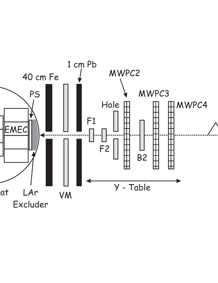
Figure 1: Schematic view of the general beam test set-up. Shown are the modules in the cryostat as well as the beam instrumentation used.

The load in the liquid argon (LAr) cryostat consists of the outer section of one EMEC module (1/8 of the full EMEC wheel), three HEC1 modules (3/32 of the full HEC1 wheel) and two HEC2 modules. Constrained by the cryostat dimensions the depth of the HEC2 modules was half of the ATLAS modules. The impact angle of beam particles was $90^{\circ}$ with respect to the front plane, yielding a non-pointing geometry of the set-up in $\eta$ (vertically) unlike the ATLAS situation. Fig. 1 shows the location of the trigger and veto counters. The trigger is derived from the scintillation counter B1, three scintillator walls VM, M1, M2, and two scintillation counters F1, F2 (pretrigger, for details see [3]) for fast timing. Up to $80\,\mathrm{GeV}$ the Cherenkov counter was used for the event trigger as well. The impact position and angle of particles were derived from four multiwire proportional chambers (MWPC) with vertical and horizontal planes per chamber having $1\,\mathrm{mm}$ (MWPC 2, MWPC3, MWPC4) and $2\,\mathrm{mm}$ (MWPC5) wire spacing. The veto wall VM rejects beam halo particles; muons are tagged using the coincidence of M1 and M2 signals. The M1 and M2 scintillator walls are separated by an iron wall. The cryostat has an inner diameter of $2.50\,\mathrm{m}$, it can be filled with LAr up to a height of $2.20\,\mathrm{m}$. It can be moved horizontally by $\pm 30\,\mathrm{cm}$. The beamline vertical bending magnet allows the beam to be deflected in a range of $\pm 25\,\mathrm{cm}$ at the front face of the cryostat. The circular cryostat beam window has a reduced wall thickness ($5.5\,\mathrm{mm}$ stainless steel) and a diameter of $60\,\mathrm{cm}$. Thus an area of $60\times 50\,\mathrm{cm}^{2}$ is available for horizontal and vertical scans. The calorimeter modules in the cryostat are shown in Fig. 2.

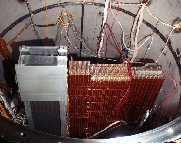
Figure 2: Top view of the cryostat, showing (from left to right) the EMEC module with the presampler, the three HEC1 modules and the two HEC2 modules of reduced longitudinal size.

The top view of the cryostat shows (from left to right) the EMEC module including the presampler, the three HEC1 modules and the two HEC2 modules of reduced longitudinal size. Simulation studies show that the typical leakage for pions is at the level of $4$-$6\,$% (see section Monte Carlo simulation). Monitoring of the LAr purity and temperature are included in the cryostat; details may be found in [3].

2.3 Read-out Electronics and Data Acquisition

The HEC cold front-end electronics was identical to the one used in the previous HEC stand-alone tests [3]. The output signals of the cold HEC summing amplifiers as well as the raw signals from the EMEC were carried to the front-end boards (FEB) outside the cryostat. Here the amplification of the EMEC signals and signal shaping of all signals was performed. The crate with the FEB’s was directly located on the two related feedthroughs, thus extending the Faraday cage of the cryostat. The signals were sampled and stored in the switched capacity array of the FEB at a rate of $40\,\mathrm{MHz}$. Upon arrival of the trigger the FEB’s stopped the sampling, performed the digitization and sent the data to the read-out driver (ROD) via a serial electrical link. The two types of FEB’s used for the EMEC and HEC channels are described in refs. [1, 2, 3]. The read-out of the EMEC data was performed by nine MINI-ROD modules, exploited previously for the EMEC stand-alone tests [1]. The prototype of the ATLAS ROD module (ROD-demo [5]), designed to validate the final ATLAS-LAr calorimetry read-out system, was used for the HEC read-out. The ROD-demo was a 9U VME motherboard with four mezzanine processing unit (PU) cards. Each PU processed the data from one half FEB, so in total six PU’s on two ROD boards were used to read out the three HEC FEB’s.

The triggering and the synchronization of the nine EMEC FEB’s and the three HEC FEB’s as well as the nine MINI-ROD’s, two ROD-demo modules and two calibration boards was done using the TTC-0 system as employed in the EMEC stand-alone tests [1]. In addition, a simple level converter adapted the TTC-0 signals to the ROD-demo standard. The relative timing of the pre-trigger (see [3] for details) with respect to the $40\,\mathrm{MHz}$ sampling clock was logged by a TDC module. The beam trigger scintillation counters and the related fast logic as well as the multiwire proportional chambers used for tracking the beam particles were identical to those previously used in the HEC stand-alone test [3]. The block diagram of the front-end, read-out and trigger electronics is shown in Fig. 3.

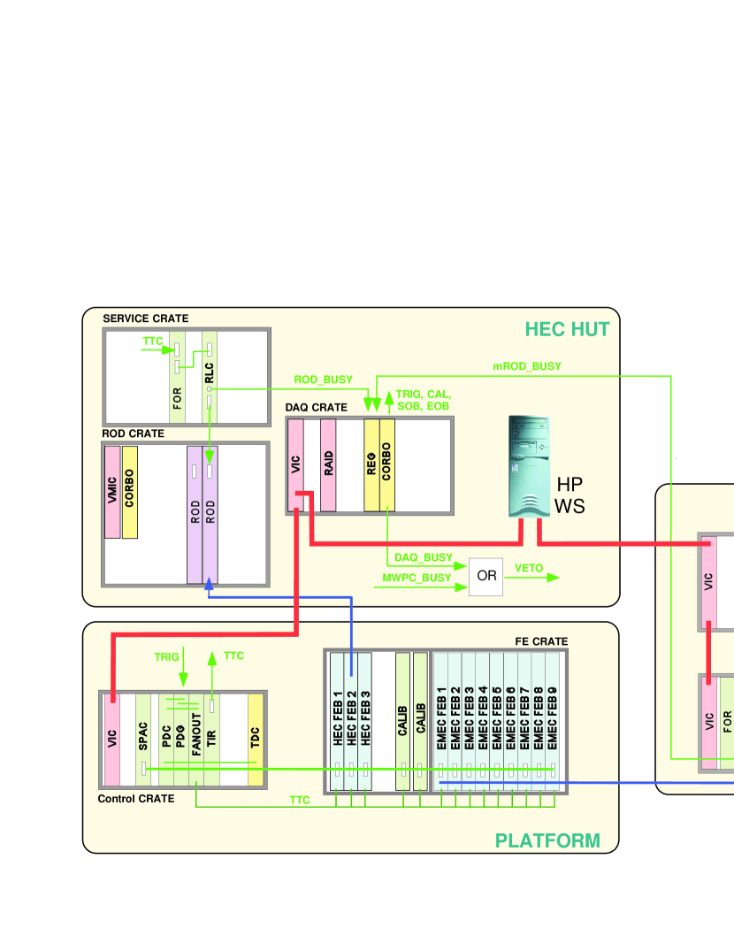
Figure 3: Block diagram of the front-end, read-out and trigger electronics.

The data acquisition system included a 6U control crate with the TTC-0 system and the TDC module, located near the front-end crate on the cryostat platform. The 6U crate with the MINI-ROD modules and the 6U service crate were placed in the EMEC control room. All other components of the system, the 9U crate with the ROD-demo boards, the CAMAC crate with the MWPC read-out, the 6U crate with the registers for the scintillation counters and the event builder (CES RAID module with a RISC CPU, running the real time system CDC EP/LX) were in the HEC control room.

2.4 Calibration and Signal Reconstruction

The signal was sampled every $25\,\mathrm{ns}$. Five samplings were typically used to reconstruct the full amplitude. For the EMEC typically 7 samplings have been read-out. For the HEC, where due to the larger read-out cell capacities in comparison to the EMEC a larger noise is expected, usually 16 samplings have been used. Here the first samplings were preceding the pulse, so the noise could be reconstructed the same way as the signal amplitude. But for signal shape studies even a larger number of samplings has been used.

The hardware calibration system used was the same as in the previous HEC stand-alone beam test runs [3]. For the HEC the calibration pulse is injected directly at the pad, for the EMEC at the motherboards. Therefore the procedure used for the signal reconstruction and the prediction of the calibration parameters was different for the HEC and EMEC and is described briefly here.

Because the optimal filtering method for amplitude reconstruction [6] will be used in ATLAS, we followed the same procedure in the beam test calibration. A detailed knowledge of both the amplitude response and the waveform dependence on the amplitude is needed. The goal of the optimal filtering method is to reconstruct the amplitude and time of a signal with a known signal shape from discrete measurements of the signal. Thus the method minimizes the noise contribution to the amplitude reconstruction.

To unfold the particle signal shape from the calibration signal shape an inverse Laplace transformation has been used for the HEC and a Fourier Transformation for the EMEC. This choice is mostly driven by the difference in the injection of the calibration pulse. For each method we stay within the traditional set of variables, e.g. $s=j\omega$, with $\omega$ being the angular frequency.

2.4.1 HEC calibration

For the HEC signal reconstruction a new procedure, compared to previous beam test runs [3, 7], was applied, using the detailed knowledge of the electronic chain. The full response function in the beam test set-up can be written in the frequency domain (multiplicative constants not included) as ($\tau_{x}$ are various time constants and $\alpha$ is the parameter of the calibration current shape $I^{\rm cal}(t)=\alpha+(1-\alpha)e^{-t/\tau_{\rm cal}}$):

$$H(s) = \frac{\alpha+s\tau_{\rm cal}}{s\cdot(1+s\tau_{\rm cal})}\cdot\frac{(1+s\tau_{\rm zc})(1+s\tau_{\rm sl})}{(1+s\tau_{\rm pc})(1+s\tau_{\rm 0c})}\times$$

$$\frac{1}{(1+s\tau_{\rm a})(1+s\tau_{\rm d})}\cdot\frac{(1+s\tau_{\rm zs})}{(1+s\tau_{\rm ps})(1+s\tau_{\rm 0s})}\times$$

$$\frac{(1+s\tau_{\rm pz})}{(1+s\tau_{\rm i})(1+s\tau_{0})}\cdot\frac{s\tau_{\rm s}}{(1+s\tau_{\rm s})^{3}\cdot(1+s\tau_{\rm fd})\cdot(1+s\tau_{\rm ac})},$$

where the first line corresponds to the calibration generator chain ($H^{\rm c}(s)$), the second line to the cold electronics and cables, and the third line to the warm electronics part ($H^{\rm e}(s)$). This function cannot be generated in time domain by directly performing an inverse Laplace transformation (ILT). Instead we made use of the well known method of ILT for rational functions, known as the expansion to poles, based on the fact that any rational function can be expanded as ($n>m$, all poles are different):

$$\frac{(s+z_{1})\cdot(s+z_{2})\ldots(s+z_{m})}{(s+p_{1})\cdot(s+p_{2})\ldots(s+p_{n})}\equiv\sum_{k=1}^{n}\frac{d_{k}}{s+p_{k}}.$$

The values $d_{k}$ are determined by zeros and poles, and can be calculated numerically. Then the ILT becomes,

$$\sum\frac{1}{s+p_{k}}\Rightarrow\sum{\rm e}^{-p_{k}\cdot t}.$$

This method can be applied separately to the calibration signal $H^{\rm c}(s)$ with $N_{\rm c}$ poles, and to the electronic chain response function $H^{\rm e}(s)$ with $N_{\rm e}$ poles, so that

$$H^{\rm c}(s)=\sum_{i=1}^{N_{\rm c}}\frac{C_{i}}{1+s\cdot S^{\rm c}_{i}};~{}~{}~{}~{}~{}H^{\rm e}(s)=\sum_{i=1}^{N_{\rm e}}\frac{E_{i}}{1+s\cdot S^{\rm e}_{i}},$$

where $S^{\rm c}_{i}$ are all poles of $H^{\rm c}(s)$ and $S^{\rm e}_{i}$ are all poles of $H^{\rm e}(s)$. Using the property of convolution of two exponential functions

$${\rm e}^{-s_{1}\cdot t}\otimes{\rm e}^{-s_{2}\cdot t}\equiv\frac{{\rm e}^{-s_{1}\cdot t}-{\rm e}^{-s_{2}\cdot t}}{s_{2}-s_{1}},$$

the calibration signal is the combination of exponential functions:

$$U^{\rm c}(t)=\sum_{i=1}^{N_{\rm c}}\sum_{j=1}^{N_{\rm e}}E_{j}\cdot C_{i}\cdot\frac{{\rm e}^{-S^{\rm c}_{i}\cdot t}-{\rm e}^{-S^{\rm e}_{j}\cdot t}}{S^{\rm e}_{j}-S^{\rm c}_{i}}.$$

The measured calibration signal shape was fitted with two free parameters, namely the $\tau_{\rm s}$-shaper pole and $\tau_{\rm pz}$-preshaper pole. Other parameters are known from laboratory measurements of the electronic chain. We computed $C_{i}$ analytically (2 zeroes and 3 poles), and $E_{j}$ during numerical fitting resolving the system of $n$ linear equations. To be able to use the method we approximated by substituting the triple pole for the shaper by three single poles with very close time constants ($\pm 0.1\,\mathrm{ns}$). The result of the fit for one HEC channel is shown in Fig. 4.

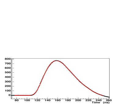
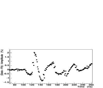
Figure 4: For a typical HEC read-out channel: Left: the measured calibration signal (points) fitted by the full electronics function (line). The amplitude is shown in units of ADC counts. Right: the residua of the fit.

The left figure shows the calibration signal (points) fitted by the full electronics function (red line). The right figure shows the corresponding residua of the fit. The residua are well within $\pm 1.5\,$%, except for the signal rise, where the influence of small distortions of the calibration pulse shape is not taken into account.

The fitted parameters of the response function were used to predict the ionization current by convolution of $H^{\rm e}(s)$ with the triangle current where the only free parameter is the drift time. The predicted function was used to compute the optimal filter weights [6]. The comparison of the pion data with the predicted particle shape for the same HEC channel is shown in Fig. 5.

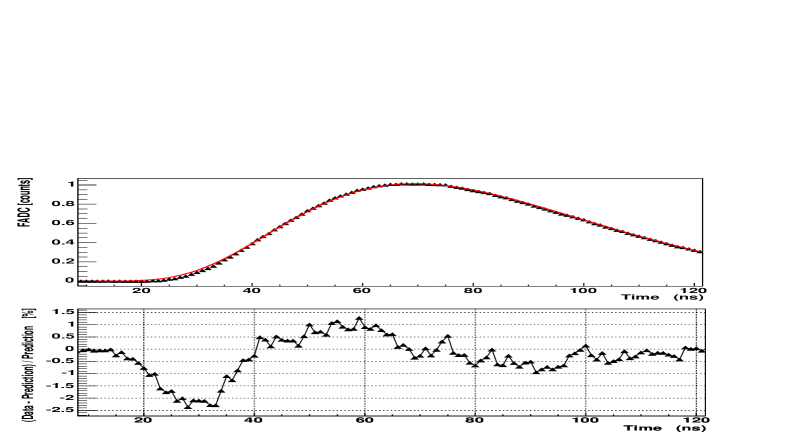
Figure 5: Upper figure: comparison of the measured normalized particle signal (points) with the prediction (line) using the parameters as obtained from the fit of the calibration signal. Lower figure: corresponding residua.

The upper figure shows the comparison of the measured normalized particle signal (points) with the prediction (line) using the parameters as obtained from the fit of the calibration signal. The lower figure shows the corresponding residua. Apart from near the signal start, where the influence of calibration pulse imperfections is seen, the shape is predicted again rather well (residua within $\pm 1.5\,$%). In summary, the precision of the resulting signal reconstruction of real particles, is at the level of $\pm 1\,$%.

Finally the transformation of the measured amplitude from voltage to current was done using a 3^rd order polynomial or a linear function. The coefficients of the polynomial were computed in two steps:

• the calibration signals with different currents were transformed to triangular signals corresponding to the same currents;

• the resulting amplitudes were fitted by the calibration polynomial to obtain the coefficients $p_{i}$ for the transformation of the amplitude $A$ to current $I$: $I=\sum_{i=0}^{n}p_{i}\cdot A^{i}$, with $n=3$ typically.

2.4.2 EMEC calibration

In comparison to the HEC, for the EMEC the electronic paths of the calibration signal and of the particle-induced signal are more complicated, and therefore a different approach was used to calibrate the EMEC. In addition to the main difference between the calibration pulse shape (exponential function) and the particle shape (triangle), there is also a substantial inductive and capacitive difference between the two paths.

The particle pulse shape can be predicted from the calibration pulse shape by applying two transformations, one for the current signal shape and the other for the injection point:

$$H^{\rm cur}(s)=\frac{I^{\rm phy}(s)}{I^{\rm cal}(s)}=\frac{(st_{\rm dr}+e^{-st_{\rm dr}}-1)(1+s\tau_{\rm cal})}{st_{\rm dr}(\alpha+s\tau_{\rm cal})},$$ (1)

$$H^{\rm lc}(s)=\frac{H^{\rm phy}(s)}{H^{\rm cal}(s)}=\frac{1}{1+sRC+s^{2}LC},$$ (2)

where $t_{\rm dr}$ is the drift time, $\tau_{\rm cal}$ and $\alpha$ are parameters of the calibration current shape, and $I^{\rm cal}(t)=\alpha+(1-\alpha)e^{-t/\tau_{\rm cal}}$.

In this calculation, we assume that the calorimeter read-out pad behaves as a simple capacitor $C$, and that the strip-line on the detector between the pad and the summing board (where the calibration signal is injected) can be modeled with a series inductor $L$, and series resistor $R$. The model circuit used in the method is shown in Fig. 6.

The method is based on a technique developed previously for the ATLAS electromagnetic calorimeters [8, 9]. The particle-induced signal pulse shape is predicted from the calibration pulse shapes using the Fast Fourier Transform (FFT) in the following steps :

• Signal pulse shapes are obtained by averaging many pulses in each channel in high energy pion and electron runs. Since the sampling time in each channel is $25\,\mathrm{ns}$ but $1\,\mathrm{ns}$ bins are used in the pulse shapes, there is a set of bin-to-bin statistical normalization constants, which are initially assumed to be unity;

• Extrapolate the calibration pulse (800 time samples) smoothly by using an exponential function to avoid the discontinuity at the edges of the time window, expanding the time window to 2048 time samples;

• Apply a FTT to this expanded calibration pulse, to transform it into the frequency domain;

• Apply the two transformations to the calibration pulse shape in the frequency domain, and then convert it to the time domain with the FFT. This is the “predicted physics signal” in the time domain;

• Calculate the free parameters ($LC$, $RC$ and the drift-time) using $\chi$-square minimization.

The above calculation was repeated for different signal pulse shape bin-to-bin normalizations until the fit converged.

This procedure provides a pulse shape for each channel from the calibration signal that is suitable for use in providing optimal filtering weights for analyzing physics pulses in the channel. More importantly, it also gives predictions for $LC$ and $RC$, which are needed to compute the absolute normalization of the signal pulses in units of ionization current using the calibration system. All cells were not scanned during the beam test runs, and therefore there are some cells without valid signal pulse shapes. Signal pulse shapes from cells with similar characteristics are used for cells without a signal pulse shape.

The optimal filtering coefficients are applied to 5 pulse samples with $25\,\mathrm{ns}$ spacing. Because the beam particles arrive at the calorimeter asynchronously with respect to the $40\,\mathrm{MHz}$ clock, only a fraction of the pulses are actually sampled near the peak. The expected reconstructed pulse height is defined to be that of an ideal continuous pulse passing through these samples. The quality of the signal reconstruction is assessed by taking a large sample of events with hits in a channel, and plotting the average value of the sample in a given time bin normalized event-by-event to the reconstructed pulse height. Because this average pulse is reconstructed for many pulses with different sampling times, the complete average pulse can be reconstructed with fine time bins, and is shown for one example channel in Fig. 7. If the optimal filtering weights are correct, the observed height of this normalized plot should be unity. The check verifies that the pulse height is reconstructed to better than $1\,$% accuracy.

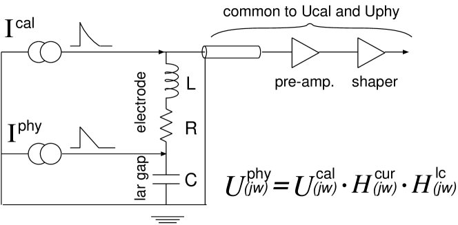
Figure 6: Schematic EMEC read-out chain and calibration network. The variables $U^{\rm phy}(j\omega)$ and $U^{\rm cal}(j\omega)$ are the pulse shapes in the frequency domain for the physics and calibration pulses, respectively.

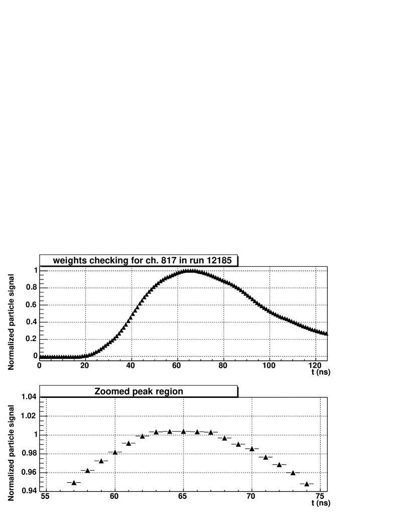
Figure 7: Upper figure: normalized particle signal, using optimal filter weights computed from the calibration signal. Lower figure: close up of the peak region.

3 Data Analysis

3.1 Data

In total 743 runs have been taken with electrons, pions or muons in the energy range $6\,\mathrm{GeV}\leq E\leq 200\,\mathrm{GeV}$ with about 25 million triggers in total. The data for the energy scans have been taken typically at 9 beam impact points. They are shown in Fig. 8, projected onto the front face of the three HEC1 modules. Shown is also the related pad structure, the projection of the beam window (circle) and the position of the calorimeter tie rods (open circles).

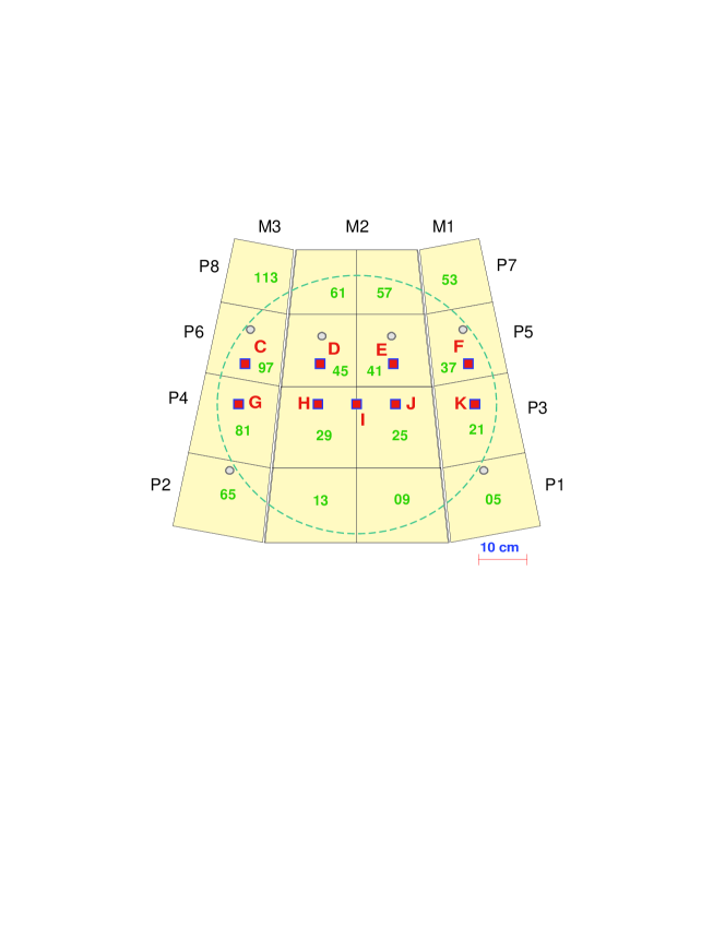
Figure 8: Position of the beam impact points (C-K) on the front face of HEC1. The large circle indicates the beam window; the small circles the position of the tie rods

The lower row (G-K) corresponds roughly to an $\eta$-range of $1.51$ (PS) - $1.65$ (layer 3) for the EMEC and to $1.67$ (layer 1) - $1.87$ (layer 3) for the HEC, the upper row (C-F) to $1.55$-$1.67$ (EMEC) and to $1.72$-$1.92$ (HEC) respectively. Horizontal and vertical scans have been performed for all particle types and at various beam energies. In the region of the cryostat window the amount of dead material in front of the calorimeter is minimal, about $0.6\,X_{0}$ in total. To study the variation of the response in the presampler, EMEC and HEC modules with dead material in front, dedicated scans have been done introducing varying amounts of additional dead material in front of the cryostat.

3.2 Electronic Noise

The optimal filtering (OF) method minimizes the noise-to-signal ratio for the signal reconstruction using the known particle signal shape and the resulting noise autocorrelation weights. Figs. 9 and 10 show the RMS noise of the pedestal (using optimal filtering) for the individual read-out channels of the EMEC and HEC. For the HEC a special channel numbering has been used (given in the Figure) to map the read-out channels $\rm{i}$ to the layer structure of the HEC. The variation of the noise is as expected from the related channel capacitance. For the EMEC the groups of channels in layer 0 (presampler) and layer 1, 2 and 3 are clearly visible. For the HEC the capacitance variation that depends on $\eta$ can be seen. It is structured into individual bands related to the corresponding longitudinal segment. For more details see [10].

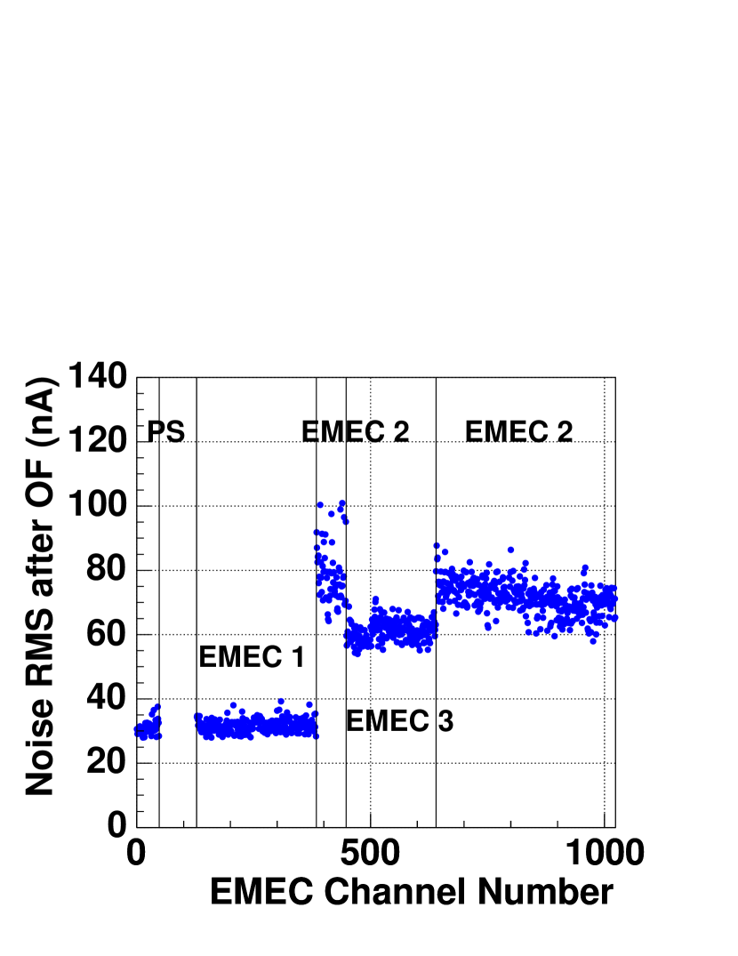
Figure 9: Electronic noise in the EMEC: shown is the RMS noise of the pedestal (after optimal filtering) for the individual read-out channels

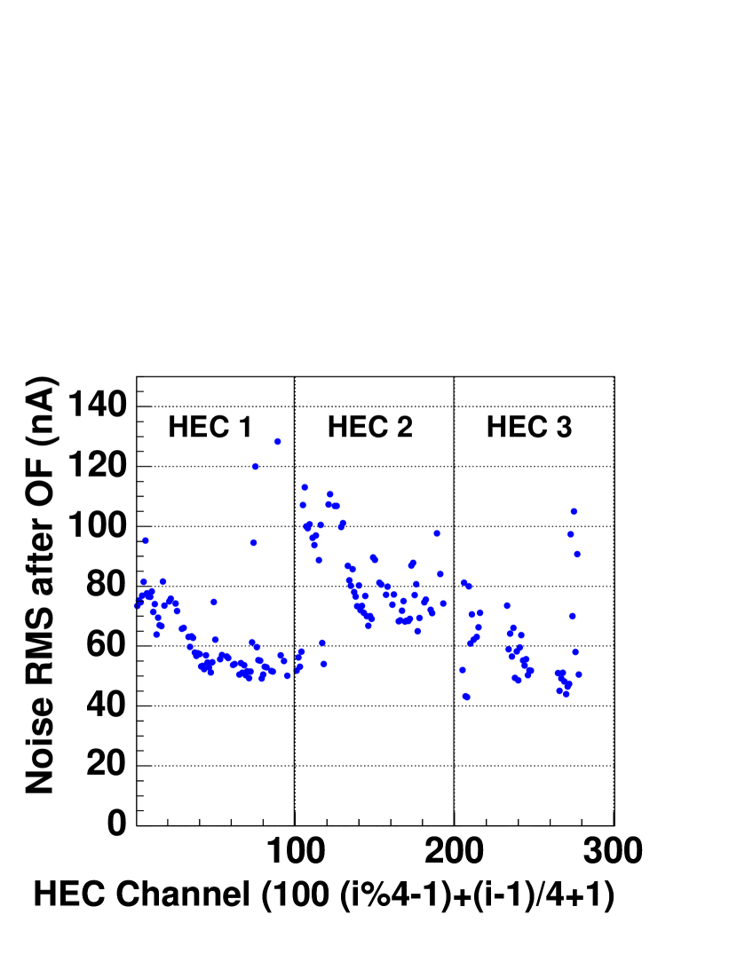
Figure 10: Electronic noise in the HEC: shown is the RMS noise of the pedestal (after optimal filtering) for the individual channels. A special channel numbering has been used to map the read-out channels $\rm{i}$ to the layer structure of the HEC.

For the EMEC data only the very first time sample is preceding the signal pulse. Therefore the impact of the OF method on the noise has been studied using the muon data. Here only the channels hit directly by the muon had to be excluded. Fig. 11 shows the corresponding result for the EMEC channels. The noise is normalized to the related pedestal RMS of the corresponding channel. From the fit a $\sigma$ of about $69\,$% of the pedestal RMS was obtained, showing that the OF result is somewhat worse than theoretically expected (see HEC below). The quality of the prediction of the signal pulse shape as well as residual coherent noise seem to set some limitation.

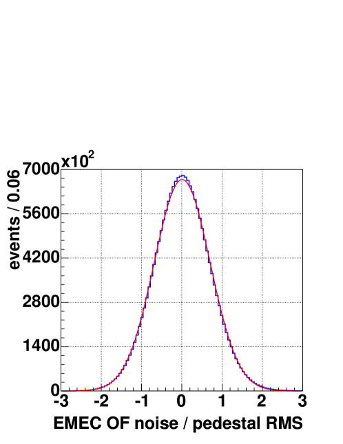
Figure 11: Pedestal subtracted signal of individual EMEC channels with no energy deposition as obtained from OF reconstruction. This noise is shown in units of the pedestal RMS. The histogram shows the data; the line is a gaussian fit to the distribution.

Figure 12: Pedestal subtracted signal of individual HEC channels with no energy deposition as obtained from OF reconstruction. This noise is shown in units of the pedestal RMS. The histogram shows the data; the line is a gaussian fit to the distribution.

For the HEC data, where the first time samples are preceding the signal pulse, the first five time samples have been used to obtain the noise on an event by event basis after applying the OF weights. Fig. 12 shows the pedestal noise of individual HEC channels as obtained from the OF reconstruction. The noise obtained is given in units of the pedestal RMS. The histogram shows the data, the line is a gaussian fit to the distribution. From the fit a $\sigma$ of about $60\,$% of the pedestal RMS can be obtained, demonstrating a noise reduction by the OF method of $\sim 1.7$. This is exactly the value theoretically expected for five samplings used in the amplitude reconstruction. It also shows that any coherent contribution to the noise is very low, and that the signal shape reconstruction is well modeled.

3.3 Online Monitoring and Offline Software

For this EMEC/HEC combined run the analysis and monitoring software were integrated into the ATLAS object-oriented C++ ATHENA framework in contrast to the previously used software [11]. This software package includes tools for decoding the online data, building data ’objects’, storing them in the ATHENA transient data store, and finally developing all analysis tools within the ATHENA framework. This new software package has many benefits. In particular, the software being developed for beam test calibration, monitoring and analysis will be directly available for analysing eventual ATLAS data, encouraging the transfer of expertise from the detector groups leading the beam test effort into the offline software and analysis. The implementation of the beam test analysis into ATHENA, its first application to real data, is currently driving a number of significant modifications to the ATLAS software and analysis framework. These modifications include many features allowing ATHENA to cope with real conditions such as imperfect time varying data with changing calibration constants and detailed event data content. The EMEC/HEC combined beam test was the first use of ATHENA for beam test analysis, and the expertise gained in this effort is being carried forward into upcoming beam tests and offline analysis.

3.4 Global Event Timing

In contrast to the ATLAS situation at the LHC, the trigger in the beam test is asynchronous with respect to the $40\,\mathrm{MHz}$ clock. The relative timing between the clock and the trigger can be defined using either the TDC information or it can be derived from global event timing. From a 3^rd order polynomial fit to the signal shape of an individual channel $i$ with a significant pulse height the ‘cubic time’ $t_{i}$ can be derived. Mainly due to differences in cabling the timing of individual channels varies by up to $\pm 10\,\mathrm{ns}$ for the EMEC and $\pm 3\,\mathrm{ns}$ for the HEC. These channel offsets have been defined from a global fit minimizing the channel-to-channel time differences for all EMEC and HEC channels over all electron and pion runs. Knowing these offsets $\Delta t_{i}$ finally a ’global cubic time’ for each event can be determined with:

$$t_{\rm global}=\frac{\displaystyle\sum_{i}{\left[t_{i}-\Delta t_{i}\right]/\sigma_{t,i}^{2}}}{\displaystyle\sum_{i}{1/\sigma_{t,i}^{2}}},\qquad{\rm with}\quad\sigma_{t,i}=\frac{24.1\,\mathrm{ns}}{{\rm signal}_{i}/\sigma_{{\rm noise},i}}\oplus 0.55\,\mathrm{ns}.$$

Fig. 13 shows the comparison of the global time $t_{\rm global}$ thus obtained but without using the channel with the largest signal with the cubic time of the channel with the largest signal over all runs. The precision of the global time $t_{\rm global}$ is better than $1.5\,\mathrm{ns}$. The slight offset from zero might be partially related to the time evolution of the shower development, which is for the hottest channel the shower core and for other channels more in the shower tail.

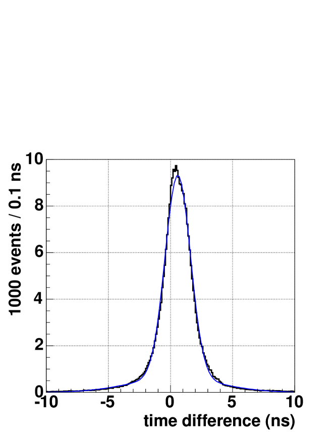
Figure 13: Time difference: comparison of the global time $t_{\rm global}$ with the cubic time of the largest signal channel.

3.5 Cluster Algorithm

A cluster algorithm has been developed to reconstruct the energy of the beam particle. In each layer the topological neighbours of a given cell are considered: they have to share at least one common corner. A seed is chosen if the energy is significantly above the noise: $E_{\rm seed}>4\sigma_{\rm noise}$. The general cut-off at the cell level is $|E_{\rm cell}|>2\sigma_{\rm noise}$, the cluster is expanded with neighbours of all cells satisfying $|E_{\rm neighbour}|>3\sigma_{\rm noise}$. Symmetric cuts have been chosen in order to avoid major energy offsets due to noise pick-up. Fig. 14 shows the read-out cells of a typical $148\,\mathrm{GeV}$ electron event: in total there are four EMEC clusters (one per layer) and no HEC clusters with 83 channels in total. Due to the non pointing geometry and the different cluster algorithm used, the cluster size obtained for electrons is bigger than the corresponding one used in the EMEC modules 0 analysis.

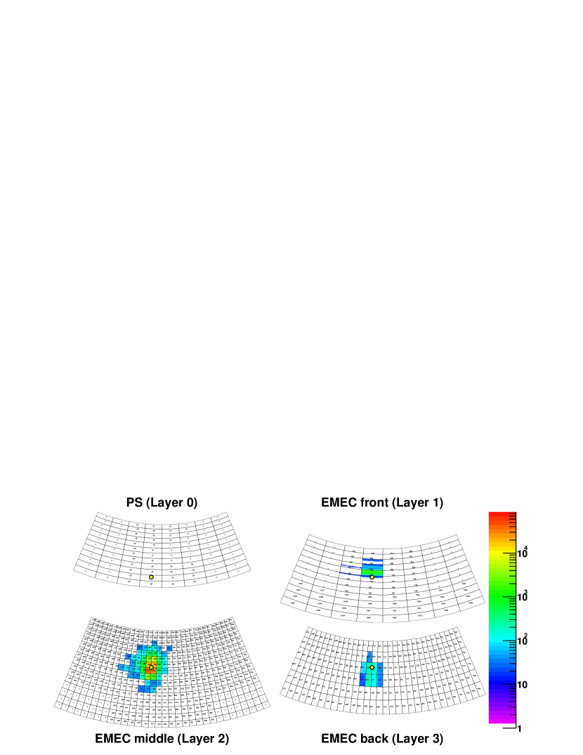
Figure 14: Reconstructed EMEC cluster for an electron of $148\,\mathrm{GeV}$. The yellow dot shows the beam impact point; the scale is given in nA.

For a typical pion of $180\,\mathrm{GeV}$ the corresponding distribution of read-out cells selected is shown in Figs. 15 and 16: in total there are six clusters in the EMEC with 128 channels and three HEC clusters with 11 channels.

Figure 15: Reconstructed EMEC clusters for a pion of $180\,\mathrm{GeV}$. The yellow dot shows the beam impact point; the scale is given in nA.

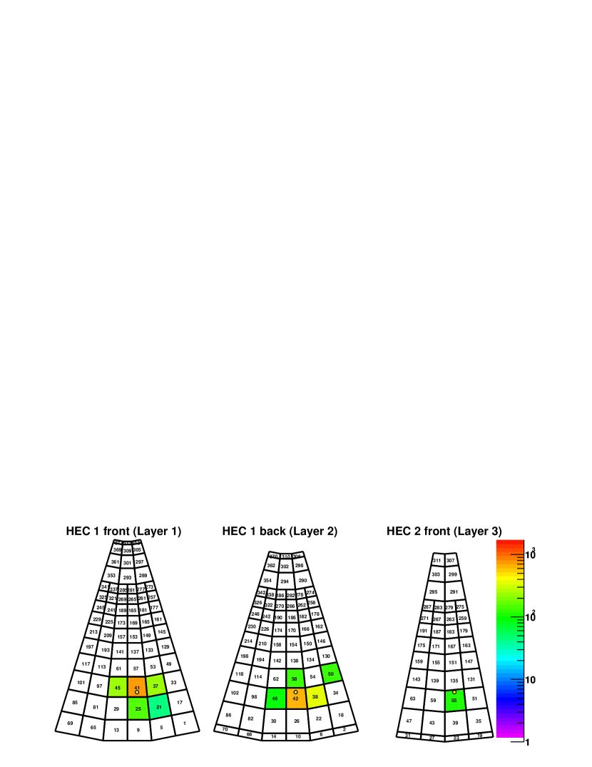
Figure 16: Reconstructed HEC clusters for a pion of $180\,\mathrm{GeV}$. The yellow dot shows the beam impact point; the scale is given in nA.

The colour code indicates the related signal height of the individual read-out cells. The cluster algorithm proves to be very efficient for the reconstruction of the particle energy deposited and avoids including too much noise in the particle signal.

3.6 Alignment

In ATLAS the three sub-detectors EMEC, HEC1 and HEC2 form three wheels, which are placed in one common cryostat. In the beam test set-up the relative positions of the three sub-detectors follow the ATLAS dimensions within tolerance (typically tolerances are $<3\,\mathrm{mm}$). Nevertheless, to be able to simulate details of the shower formation and cluster reconstruction, a precise horizontal and vertical alignment of the sub-detectors is required. Using the track reconstruction based on the MWPC data, the signal response in the EMEC, HEC1 and HEC2 can be closely followed in horizontal and vertical scans. Module and pad boundaries as well as tie-rod positions can be used to extract the required information with high precision. As an example, Figs. 17 and 18 show the relative response for pions of $200\,\mathrm{GeV}$ in the second EMEC layer and in the second HEC1 layer when running a horizontal scan. Plotted is in each case the ratio between the maximum signal cell response and the corresponding cluster energy. The pad boundaries are clearly visible. Using the combined information of all these data, the precision of the relative alignment is typically at the level of $\pm 1\,\mathrm{mm}$. In Fig. 18 the lateral energy leakage is visible when the beam impact approaches the outer modules: the related cluster energy is reduced.

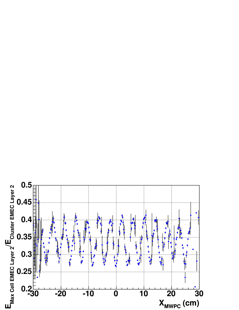
Figure 17: Signal response of pions of $200\,\mathrm{GeV}$ in the second EMEC layer from a horizontal scan as function of the beam impact position. Shown is the maximum signal in this layer with respect to the corresponding cluster energy.

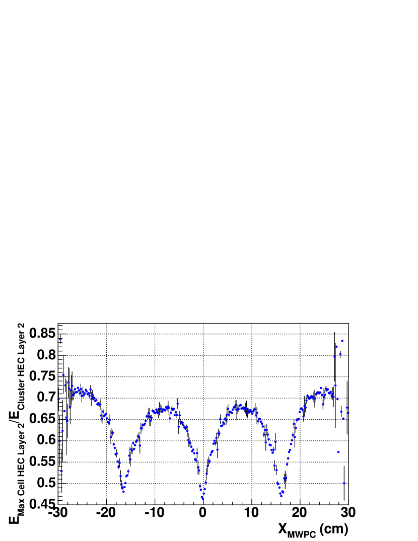
Figure 18: Signal response of pions of $200\,\mathrm{GeV}$ in the second HEC layer from a horizontal scan as function of beam impact position. Shown is the maximum signal in this layer with respect to the corresponding cluster energy.

3.7 High Voltage Corrections for Central HEC1 Module

In the second longitudinal segment of the central HEC1 module during the run one of the 4 HV lines, which are feeding the four sub-gaps of this section, had to be disconnected because of a short. The related correction 4/3 has been applied to those data. As the signal is still measured correctly in three out of four sub-gaps, all fluctuations of the hadronic shower are measured correctly as well. The main consequence due to this HV short is a reduced signal to noise ratio only. The horizontal scans with pions revealed a particular problem in the second longitudinal segment of the central HEC1 module: in particular for pions that started early showering, the response was weaker than normally. Fig. 19 shows for $200\,\mathrm{GeV}$ pions from a horizontal scan the ratio of the average energy deposited in the 2^nd longitudinal segment of the central HEC1 module over the average energy deposited in the same longitudinal segment but in the outer HEC1 modules and for different beam impact points, as function of the asymmetry of the total energy depositions in the 1^st and 3^rd (last) longitudinal segments (the last longitudinal segment being HEC2).

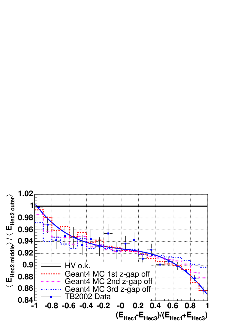
Figure 19: Ratio of the energy deposited for pions of $200\,\mathrm{GeV}$ in the 2^nd longitudinal segment of the central HEC1 module with respect to the outer HEC1 modules as function of the asymmetry of the total energy depositions in the 1^st and 3^rd (last) longitudinal segments

The effect is clearly visible and well reproduced by the MC simulation. As seen in the MC distributions, even the position of the disconnected gap can be inferred within limits, even though it is not really required. Affected were gaps at the very beginning of the 2^nd longitudinal segment. After the run this problem could be partially traced back to bad ground connections of the EST boards in this region of the central HEC1 module. To correct the data, the observed asymmetry has been determined from a fit (line). The result of this fit has been used for corrections. Thus the data have been used directly to correct for the effect observed without any further MC assumptions. Repeating this analysis for $30\,\mathrm{GeV}$ pions shows that this correction is rather energy independent. In consequence, this correction on an event-by-event basis takes care to a large extent of fluctuations in the energy deposition and thus also improves the energy resolution. This shows clearly Fig. 20: the energy resolution $\sigma/E$ for $200\,\mathrm{GeV}$ pions (electromagnetic scale) improves typically from $\sigma/E=(8.97\pm 0.12)\,$% to $\sigma/E=(8.61\pm 0.12)\,$%.

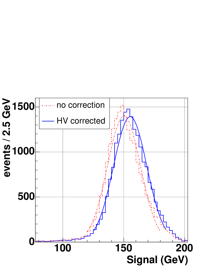
Figure 20: Energy deposition and resolution for pions of $200\,\mathrm{GeV}$ at the impact point of $x=-10\,\mathrm{cm}$ before and after the HV correction for the central HEC1 module

4 Monte Carlo Simulation

In ATLAS the final hadronic calibration is driven by jets rather than single particles. Following a weighting approach for the hadronic calibration [12] in ATLAS, weighting parameters are defined relative to the electromagnetic scale, which can be well defined in ATLAS as well as in the beam test set-up. These parameters have to be derived from MC studies. Therefore it is important that the MC describes the data well and the comparison of data with MC in the beam test is of utmost importance. Thus special software packages have been developed.

The first package uses the GEANT 3 program [13] (version 3.21) to simulate the response of various beam particles in the EMEC and HEC. The geometry description is very detailed: cryostat, liquid argon excluder, all beam elements (MWPC’s, scintillation counters etc.) as well as all details of the calorimeter modules are included. This code is based on the development done for the HEC stand-alone tests [14]. For the hadronic shower simulation the GCALOR code [15] is used. For particle tracking the threshold has been set to $100\,\mathrm{keV}$ and for secondary production of photons and electrons to $1\,\mathrm{MeV}$.

The second package uses the GEANT 4 code [16], developed by a worldwide collaboration, and since the first release in 1999 maintained by the international GEANT 4 collaboration. The implementation of the ATLAS detector including the calorimeters is still ongoing. Within this process the validation of the physics models in GEANT 4 is one of the most important tasks. From the proposed physics lists [17] for hadronic shower simulations in GEANT 4 two models have been selected for the comparison of the data with MC: LHEP and QGSP. The LHEP physics list uses the low and high energy pion parameterisation models for inelastic scattering. The QGSP physics list is based on theory driven models: it uses the quark-gluon string model for interactions and a pre-equilibrium decay model for the fragmentation. The geometrical description of the set-up is at the same level of detail as in GEANT 3. The range threshold for production has been set to $700\,\mu\mathrm{m}$ in general, irrespective of the material. This corresponds to cut-off energies of $1.03\,\mathrm{MeV}$, $1.00\,\mathrm{MeV}$ and $0.27\,\mathrm{MeV}$ for copper, lead and liquid argon respectively.

The response signals from MC simulations and data have to be compared at a well-defined scale. For the MC the inverse sampling ratio is used, that is the ratio between the electron beam energy and the total visible energy. For the HEC this ratio has been obtained from the HEC stand alone simulations as $23.3$ ($23.7$) for GEANT 3 (GEANT 4) respectively. Simulations of the combined EMEC/HEC beam test runs have been used to obtain this ratio for the EMEC. The corresponding values are $11.35$ ($12.05$) for GEANT 3 (GEANT 4) respectively. The beam test set-up causes some lateral and longitudinal leakage for hadronic showers. To evaluate the amount of leakage and its influence on the calorimeter performance, ‘virtual’ leakage detectors, placed laterally and longitudinally with respect to the EMEC and HEC modules, have been implemented in the simulations. In these ‘detectors’ the kinetic energy is summed up for all particles leaving the calorimeter modules via the related module boundaries. Figs. 21, 22 and 23 show the average fraction of energy leaking with respect to the beam energy for charged pions ($\pi^{-}$) of different energies. Shown are the results for the three MC models considered. At low energies the lateral leakage dominates, at high energies the longitudinal leakage increases. The amount of total energy leakage differs somewhat for the various MC options: GEANT 3 predicts about $6\,$%, while GEANT 4 QGSP gives $4\,$% leakage. The energy dependence of leakage is in both options rather weak. GEANT 4 LHEP is in agreement with GEANT 3 at high energies, but yields somewhat smaller leakage at low energies.

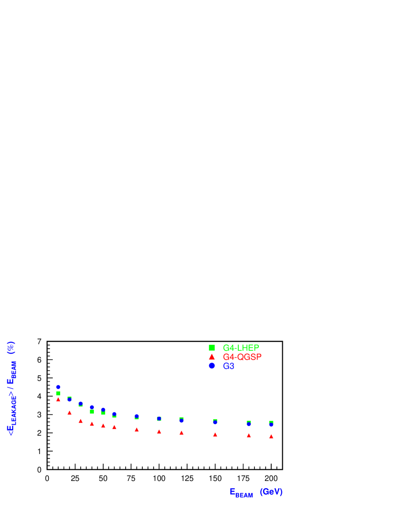
Figure 21: Energy dependence for $\pi^{-}$ of the lateral leakage for the beam test as obtained from different MC models.

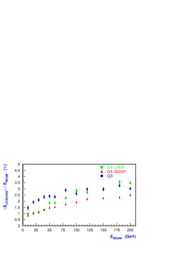
Figure 22: Energy dependence for $\pi^{-}$ of the longitudinal leakage for the beam test as obtained from different MC models.

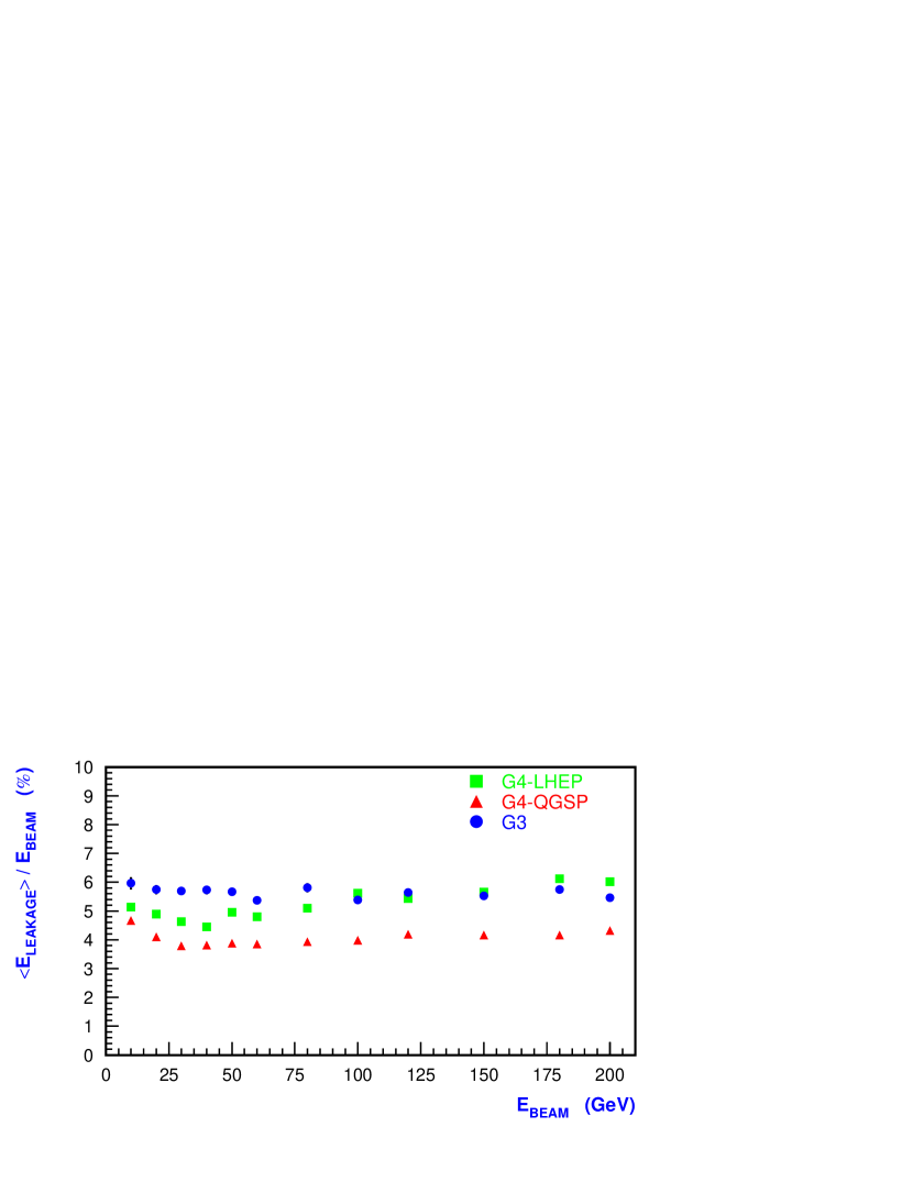
Figure 23: Energy dependence for $\pi^{-}$ of the total leakage for the beam test as obtained from different MC models.

The simulation of the noise uses real data (see section electronic noise). For the EMEC the noise has been obtained from the muon data, excluding the channels hit directly by the muon. For the HEC the first time samples are preceding the signal pulse and have been used to derive the $\sigma$ of the noise distribution.

5 Electron Results

The main goal of this beam test is the determination of the hadronic calibration – constants and procedures – in the ATLAS region of $|\eta|\simeq 1.8$. The analysis of the pion data is of most relevance for this task. Nevertheless, to be able to assess the performance of the EMEC and to obtain the electromagnetic scale, which is the basis for the hadronic calibration, the analysis of electrons is the initial step in this project. As already discussed this beam test set-up geometry is slightly non-projective, in contrast to the ATLAS detector. Thus the definitive reference for the performance of electrons in ATLAS is [1] rather than this paper. As it turns out the electron results obtained in this beam test are in close agreement to the previous analysis [1].

5.1 Corrections

The end-cap geometry of the EMEC requires small corrections [1] for the energy reconstruction of electrons. The projective HV sectors yield a variation of the signal response with $\eta$ (corresponding to $R$ in the beam test geometry). Given the limited $\eta$ range accessible in the beam test set-up and the non-pointing geometry, where the beam spread covers a larger $\eta$ range than in the pointing geometry, this variation on average is smaller in comparison to the azimuthal $\phi$ variation and has been ignored. However, electric field and sampling fraction non-uniformities as well as the non-pointing geometry, cause a significant $\phi$ variation of the signal response. Fig. 24 shows the relative response of $119\,\mathrm{GeV}$ electrons as function of $\phi$ in cell units. Here $E_{run}$ is the average energy obtained for the corresponding run.

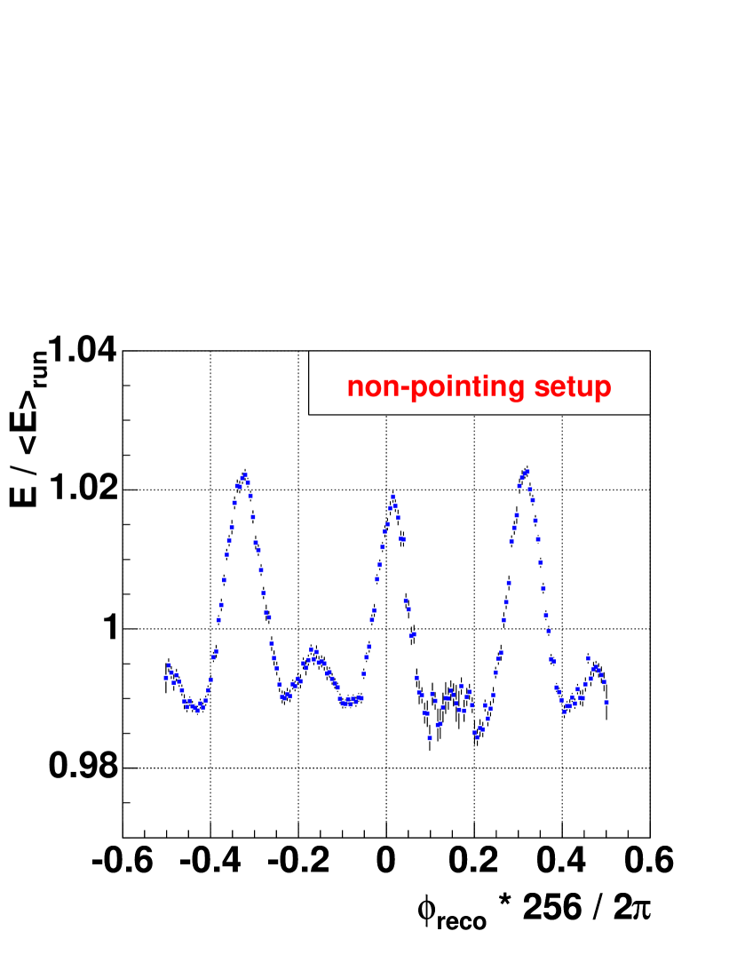
Figure 24: Relative response of electrons of $119\,\mathrm{GeV}$ as function of $\phi$. Here $\phi$ is given in units of the absorber structure spacing.

A variation at the level of $\sim\pm 1.5\,$% can be seen. A numerical correction defined bin by bin has been used for the data correction.

5.2 Energy Resolution

The energy resolution has been studied using the cluster algorithm with the corrections mentioned above. As an example Fig. 25 shows the energy resolution for impact point I.

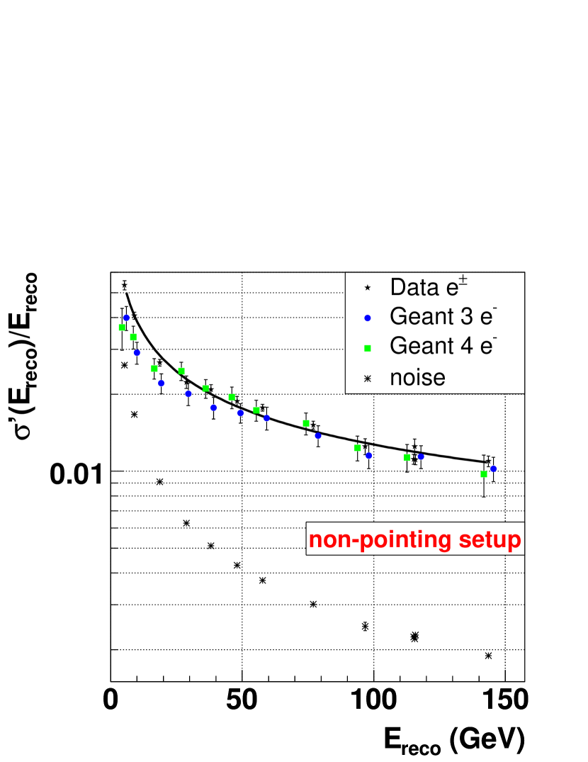
Figure 25: Energy dependence of the energy resolution of electrons for the impact point I. Shown are the noise subtracted data as well as the various MC predictions. Also shown is the noise contribution at the various energies. The line shows the result of the fit to the data.

The data have not been corrected for energy depositions outside the reconstructed cluster. The data are shown with the noise subtracted. The noise contribution is shown as well. A fit to the data (solid line) with $\frac{\sigma(E)}{E}=\frac{a}{\sqrt{E}}\oplus b$ typically yields a sampling term $a=(12.1\pm 0.2)\,$%$\sqrt{\mathrm{GeV}}$ and a constant term $b=(0.4\pm 0.1)\,$%. The GEANT 3 and GEANT 4 simulations are in good agreement and yield for GEANT 3 a sampling term of $(9.3\pm 0.6)\,$%$\sqrt{\mathrm{GeV}}$ and a constant term of $(0.8\pm 0.1)\,$% while GEANT 4 yields a sampling term of $(10.6\pm 0.7)\,$%$\sqrt{\mathrm{GeV}}$ and a constant term of $(0.7\pm 0.2)\,$% Further tuning is underway for ATLAS to improve the fair agreement with the data. For example the amplitude of the $\phi$ modulation is twice as big in GEANT 4 as in GEANT 3 and the data. Due to the beam spread this variation is corrected as for the data (see section Corrections). This causes some systematic uncertainty in the MC prediction due to the exact beam impact position and beam spread. Since the impact angle for the combined beam test is different from the geometry of the pointing EMEC stand-alone beam test [1], the energy resolution is slightly worse compared to the sampling term of $\approx 11\,$%$\sqrt{\mathrm{GeV}}$ and the constant term of $\approx 0.4\,$% obtained in the stand-alone EMEC analysis.

The energy resolution has been studied for various impact points. Fig. 26 shows the sampling term for various impact points and Fig. 27 the constant term. Because of the residual weak correlation between the constant term and the sampling term some care has to be taken when comparing the various points. Nevertheless, the differences (left and right set of points) seem to indicate some $\eta$-dependence. Partially this is related to the $\eta$-variation of the sampling fraction and also to the weak $\eta$-dependence of the electric field, which has not been taken into account.

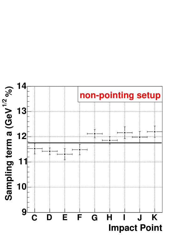
Figure 26: Energy resolution for electrons: variation of the sampling term with the impact point. The left and right set of points correspond to different $\eta$ regions.

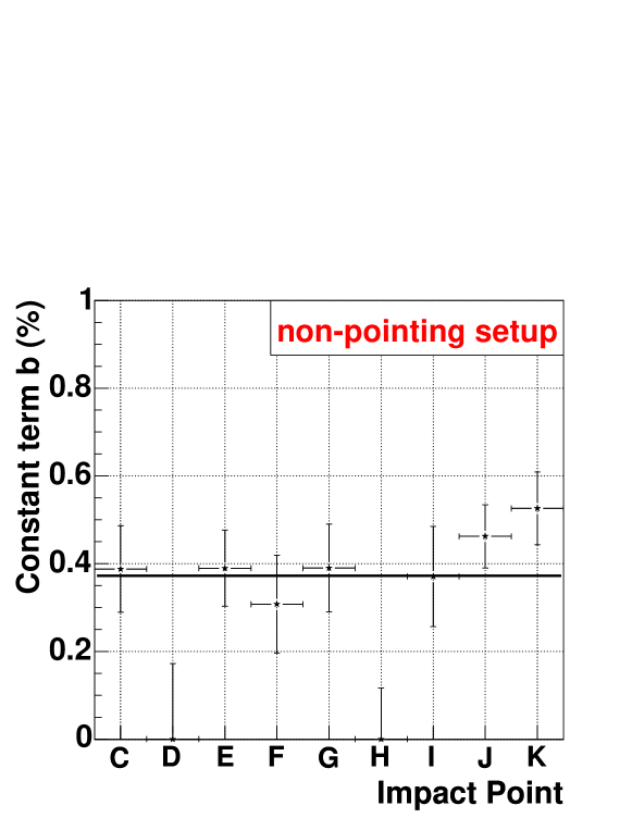
Figure 27: Energy resolution for electrons: variation of the constant term with the impact point. The left and right set of points correspond to different $\eta$ regions.

5.3 Linearity and Electromagnetic Scale

To obtain the electromagnetic scale one has to correct for the energy deposited outside the reconstructed cluster. For electrons the leakage beyond the detector boundaries is known from the MC to be negligible. The energy lost outside the reconstructed cluster can easily be obtained both for data and MC. For the energy leaking into the HEC, the electromagnetic scale of the HEC1 measured in previous HEC stand-alone beam tests can be used. For a given impact point Fig. 28 shows the relative variation of the electromagnetic scale $\alpha_{\rm em}$ with energy. In the energy range considered, the variation is typically within $\pm 0.5\,$%. Both MC models, GEANT 3 as well as GEANT 4, show a similarly good linearity of the electromagnetic scale $\alpha_{\rm em}$. The data yield an average value of $\alpha_{\rm em}=(0.430\pm 0.001)\,\mathrm{MeV}/\mathrm{nA}$. Because of the symmetric noise cuts any bias in the determination of this electromagnetic scale due to noise can be neglected. Given the uncertainty in the signal shape reconstruction ($\approx 1\,$%) and the uncertainty due to $\eta$ dependent corrections ($\approx 1\,$%), which are harder to obtain due to the non-pointing geometry and have been neglected, we attribute an overall systematic error of $2\,$% to the electromagnetic scale $\alpha_{\rm em}$, corresponding to $\pm 0.009\,\mathrm{MeV}/\mathrm{nA}$. The sampling ratio for electrons obtained from simulations depends on the model and energy and range cuts used – see the Monte Carlo simulation section.

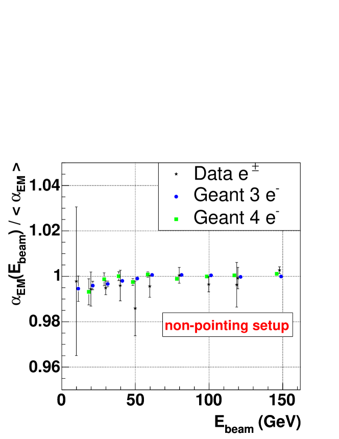
Figure 28: Linearity of the electron response: shown is the relative variation of the electromagnetic scale $\alpha_{\rm em}$ for different energies. The data are compared with MC predictions.

The fraction of the energy leakage outside the electron cluster is shown in Fig. 29.

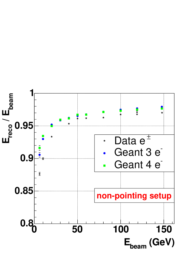
Figure 29: Fraction of energy leakage outside the reconstructed electron cluster for different energies. The data are compared with MC predictions.

Again the data are compared with MC predictions. Typically the leakage outside the cluster is between $2\,$% and $4\,$%, except for low energies. Both MC models show a somewhat smaller leakage, especially at low energies. This might be due to small effects of dead material in front of the EMEC or some cross-talk effects in the EMEC, which are not fully described in the MC.

5.4 Variation of the Response and Resolution with Material in front of the EMEC.

In ATLAS the amount of dead material in front of the calorimeter varies with $\eta$. The response in the presampler will be used to correct for the energy loss of electrons in this dead material. Therefore in this beam test electron data have been taken varying the amount of dead material in front of the cryostat. From this data presampler corrections to the measured electron energy in EMEC can be studied. The main goal of the correction is to achieve a good linearity of the electron signal, but in parallel a substantial improvement of the resolution can be obtained. Fig. 30 shows the dependence of the missing energy on the presampler signal for electrons of $10$, $20$, $119$ and $148\,\mathrm{GeV}$ with $2.73\,X_{0}$ in front of the cryostat. A 4^th order polynomial fit (solid line) to the data yields a good description of the dependence for a wide range of presampler signals and for all energies considered.

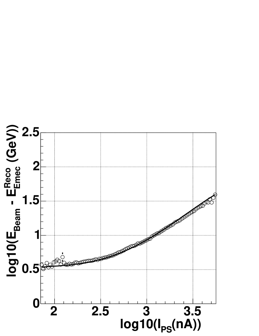
Figure 30: Dependence of the missing EMEC energy on the presampler signal for electrons of $10$, $20$, $119$ and $148\,\mathrm{GeV}$ with $2.73\,X_{0}$ in front of the cryostat. The solid line shows the result of the fit to the data.

Fig. 31 shows the ratio of the reconstructed energy relative to the beam energy as function of presampler signal for the data before (open points) and after (solid points) the correction. Again, the data for all energies studied are shown. For a wide range of presampler signals and for all energies considered the linearity of the electron signal is recovered.

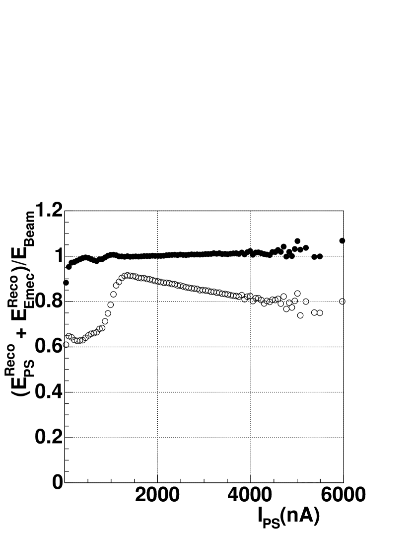
Figure 31: Electrons with additional $2.73\,X_{0}$ dead material in front of the cryostat: Ratio of the reconstructed energy over the beam energy for electrons of $10$, $20$, $119$ and $148\,\mathrm{GeV}$ before (open points) and after (solid points) the correction as a function of presampler signal.

Finally Fig. 32 shows the response of electrons of $10$, $20$, $119$ and $148\,\mathrm{GeV}$ before (dashed histogram) and after (solid histogram) the presampler corrections to the EMEC energy. Also given for each energy is the ratio of energy resolution relative to the resolution without any extra dead material in front of the cryostat: $R=[\sigma/E]_{2.73\,X_{0}}\ /[\sigma/E]_{0\,X_{0}}$. The dramatic improvement of the resolution is clearly visible: it is close to a factor of two, in particular at higher energies.

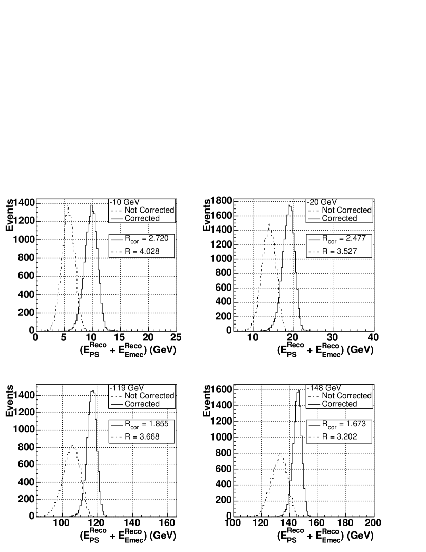
Figure 32: Response of electrons with additional $2.73\,X_{0}$ dead material in front of the cryostat for energies of $10$, $20$, $119$ and $148\,\mathrm{GeV}$ before (dashed histogram) and after correction (solid histogram). Also given is the corresponding ratio $R=[\sigma/E]_{2.73\,X_{0}}\ /[\sigma/E]_{0\,X_{0}}$ of the energy resolution relative to the resolution without any extra dead material in front of the cryostat.

It should be mentioned that an energy dependent correction could slightly improve the results. These studies, as well as the dependence on the amount of extra dead material in front, are still ongoing as part of the ATLAS energy calibration studies. However it was the goal of this analysis to restrict the corrections to a rather general and robust approach which can be further refined for ATLAS.

6 Pion Results

6.1 Response at the Electromagnetic Scale

The energy reconstruction of pions is based on the electromagnetic scale. For the EMEC value $\alpha_{\rm em}^{\rm EMEC}=0.430\,\mathrm{MeV}/\mathrm{nA}$ (see section electrons) has been used, whereas for the HEC the results from electron data taken in the previous stand-alone beam test runs [3] have been used. With respect to [3] a correction for the calibration pulse shape had to be applied, finally yielding a value of $\alpha_{\rm em}^{\rm HEC}=3.27\,\mathrm{MeV}/\mathrm{nA}$. The statistical (systematic) error of $\alpha_{\rm em}^{\rm HEC}$ is typically $1\,$% ($1\,$%). As an example, Figs. 33, 34 and 35 show the energy response in the EMEC, HEC and the total response respectively to $200\,\mathrm{GeV}$ pions at the impact point J. The data are compared with the MC predictions. Both, GEANT 3 and GEANT 4 QGSP describe the EMEC and HEC data reasonably well, even though there are some deviations visible. In contrast, the GEANT 4 LHEP simulation deviates substantially from the data both, for the EMEC and the HEC. However the GEANT 4 LHEP simulation yields the best agreement with data for the total signal.

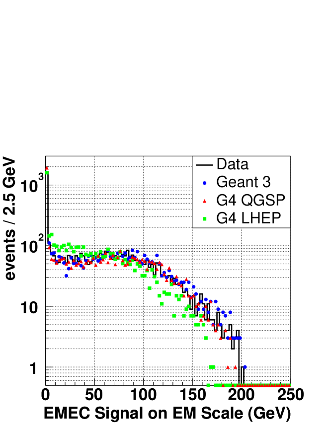
Figure 33: Response to $200\,\mathrm{GeV}$ pions in the EMEC on the electromagnetic scale. The data are compared to MC predictions.

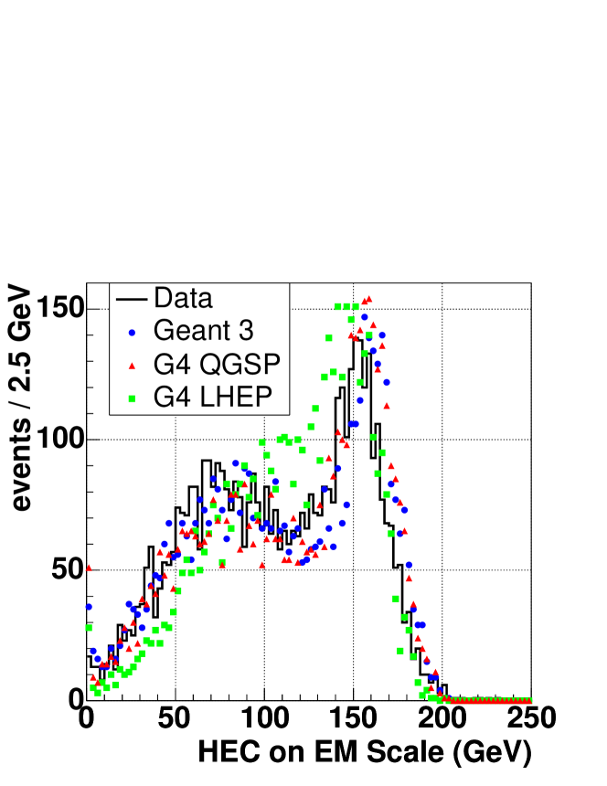
Figure 34: Response to $200\,\mathrm{GeV}$ pions in the HEC on the electromagnetic scale. The data are compared to MC predictions.

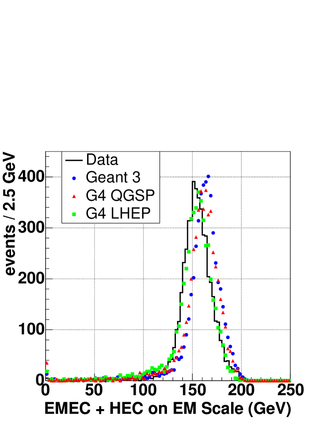
Figure 35: Total response to $200\,\mathrm{GeV}$ pions in the EMEC and HEC on the electromagnetic scale. The data are compared to MC predictions.

6.2 Energy Reconstruction using the Cluster Weighting Approach

In the ATLAS calorimeter the response to hadrons differs significantly from that for electrons of the same energy. Therefore, for hadronic energy a calibration coefficient has to be applied to the signals determined on the corresponding electromagnetic scale. The goal is to get an equal response for the electromagnetic as well as the pure hadronic component of a hadronic shower. If this goal were to be achieved fluctuations in the reconstructed hadronic shower energy could be minimized and thus the energy resolution substantially improved. The technique of signal weighting has been successfully used in previous experiments (see [18, 19] and the references therein). It exploits the fact that local energy deposits of high density are mainly due to electromagnetic interactions while for hadronic interactions the corresponding density is substantially lower. Thus for a segmented calorimeter the energy deposited in individual read-out cells can be on a statistical basis identified to be of electromagnetic or hadronic origin. For the hadronic calibration of the ATLAS calorimeter a similar approach is envisaged [12]. Methods and algorithms are still under development. The goal is to use weighting constants and weighting functions, based on the individual cluster energy, to reconstruct optimally the related energy. In ATLAS these weighting constants have to be derived from MC simulations, which to validate the method have to describe the beam test data well. The crucial MC information in this tuning process is the knowledge of the total and visible energy deposition in each read-out cell. Thus the weights could be directly derived from the MC simulation and applied to beam test data. At present this MC information is not yet available. Hence a weighting approach based on individual read-out cell energy deposits as envisaged cannot yet be achieved. Therefore a different approach has been applied.

In the EMEC and the HEC the volume of the related clusters can be used to obtain the ’EMEC cluster energy density’ and the ’HEC cluster energy density’. Here the cluster volume is the sum of all volumes of the individual cells contained in the cluster. With this information a correction to the electromagnetic scale can be derived using the information of the total energy in the EMEC and HEC on the beam energy scale. To obtain an estimate of the ‘true’ energy deposited, the energy leakage has to be subtracted from the beam energy. Energy may leak for two reasons:

• Energy deposited in the detector, but outside of the reconstructed cluster;

• Energy leaking outside the detector set-up.

The leakage outside the cluster has been obtained for each event by adding the energies (electromagnetic scale) of all readout cells not used in the cluster reconstruction. On average the noise contributions, being symmetric, cancel. Fig. 36 shows the energy dependence of this ’cluster leakage’. At low energy it rises up to $5\,\mathrm{GeV}$ and remains approximately at this level for energies above $60\,\mathrm{GeV}$. The GEANT 4 MC prediction shows a somewhat smaller leakage, the GEANT 3 prediction is closer to the data but differs in shape.

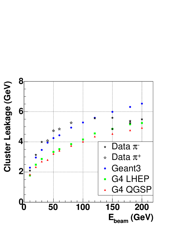
Figure 36: Energy dependence of the average energy leakage outside the reconstructed cluster for pions. Shown are the data and the different MC expectations.

To estimate the energy leakage outside the detector for each event, the MC prediction (GEANT 4 QGSP) has been used. Here the predicted correlation between the energy density (EMEC and HEC) and the energy leakage has been used. Figs. 37 and 38 show this correlation for 200 GeV pions at a particular impact point as an example. In particular for the EMEC the correlation is rather pronounced: whenever the energy density is low, leakage is getting large, separating more electromagnetic from hadronic interactions.

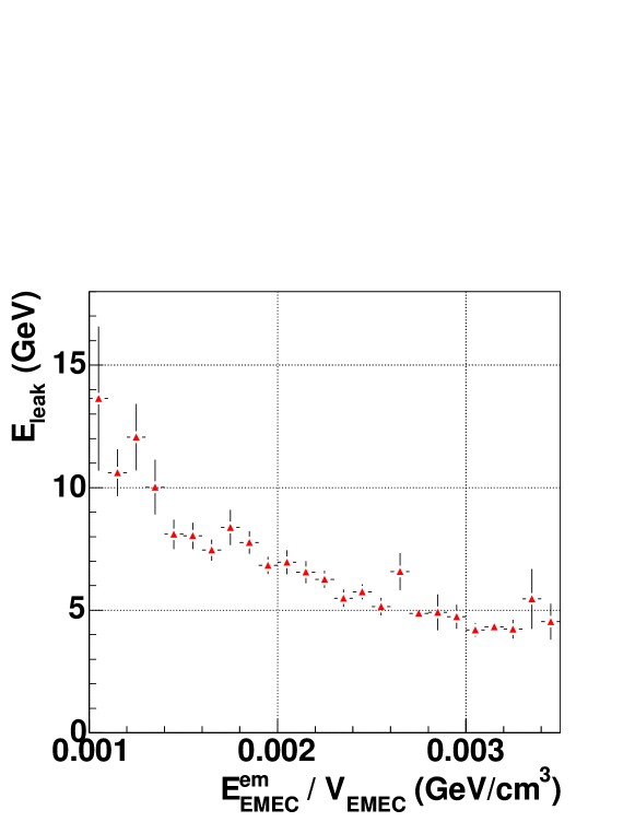
Figure 37: Correlation between the cluster energy density $E_{\rm EMEC}/V_{\rm EMEC}$ and the total energy leakage $E_{\rm leak}$ for the EMEC (at $200\,\mathrm{GeV}$).

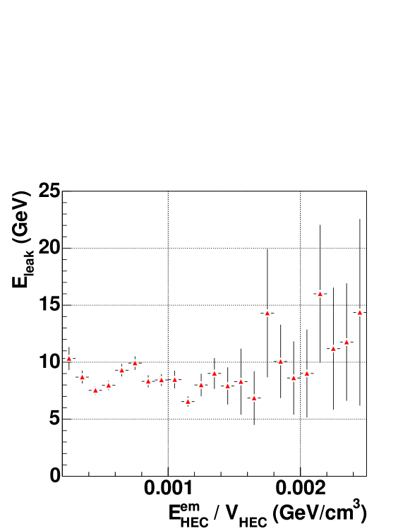
Figure 38: Correlation between the cluster energy density $E_{\rm HEC}/V_{\rm HEC}$ and the total energy leakage $E_{\rm leak}$ for the HEC (at $200\,\mathrm{GeV}$).

This total leakage is on average (see section on Monte Carlo simulation) at the level of $4\,$%.

To demonstrate this procedure $30\,\mathrm{GeV}$ pions which have deposited all their energy in the EMEC have been selected. Fig. 39 shows the ratio $w_{\rm EMEC}$ of the ‘true’ deposited energy over the measured energy on the electromagnetic scale as a function of energy density in the EMEC.

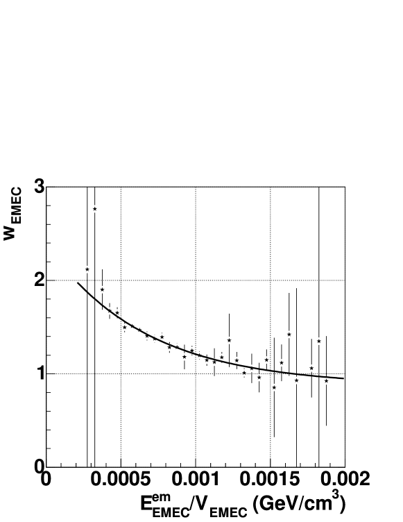
Figure 39: Ratio (’hadronic weight’) of the true energy over the energy measured on the electromagnetic scale as function of the cluster energy density for pions of $30\,\mathrm{GeV}$ fully contained in the EMEC. The line shows the result of the fit (see text).

The data can be well described using the parameterisation:

$$w_{\rm EMEC}=C_{1}\exp\left(-C_{2}E^{\rm em}/V\right)+C_{3}$$ (3)

The reconstructed energy $E^{\rm reco}$ becomes

$$E^{\rm reco}=w_{\rm EMEC}E^{\rm em}$$ (4)

where $E^{\rm em}$ refers to the EMEC cluster energy in the em scale and $V$ to the corresponding cluster volume. The fit describes the data well. The weighting parameters $C_{i}$ from the fit have been applied to the data. Fig. 40 shows the energy resolution thus obtained: weighting improves the energy resolution from $\sigma/E=26.2\,$% to $\sigma/E=15.1\,$%. The average measured energy is less than $30\,\mathrm{GeV}$ because some energy is deposited outside the cluster reconstructed ($E_{\rm leak}$).

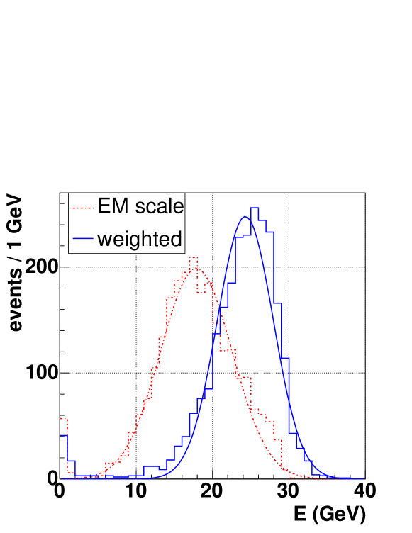
Figure 40: Comparison of energy distributions before (broken histogram and broken line) and after weighting (solid histogram and solid line) for $30\,\mathrm{GeV}$ pions fully contained in the EMEC. The energy resolution is improved from $\sigma/E=26.2\,\%$ to $\sigma/E=15.1\,\%$.

For higher energies both subdetectors, the EMEC and the HEC, have to be considered. Here a $\chi^{2}$-fit has been used to determine the parameters $C_{i}$:

$$\chi^{2}=\sum_{\rm events}\frac{{\left[E_{\rm beam}-E_{\rm leak}-E_{\rm HEC}^{\rm reco}(C_{1}^{\rm H},C_{2}^{\rm H},C_{3}^{\rm H})-E_{\rm EMEC}^{\rm reco}(C_{1}^{\rm EM},C_{2}^{\rm EM},C_{3}^{\rm EM})\right]}^{2}}{{(\sigma_{\rm noise}^{\rm reco})}^{2}+{(\sigma_{\rm noise}^{\rm leak})}^{2}},$$

where $\sigma_{\rm noise}^{\rm leak}$ is the noise contribution to the determined leakage and $\sigma_{\rm noise}^{\rm reco}$ is the integrated noise in the related cluster. The noise contribution to the determination of the energy deposits beyond the reconstructed cluster, $\sigma_{\rm noise}^{\rm leak}$, is given by the quadratic sum of the noise values on the electromagnetic scale of all calorimeter read-out cells, which are not included in the clusters. This value has been found to be rather independent of the cluster size and of the beam energy; therefore it is set to the average value of $5\,\mathrm{GeV}$. The $\chi^{2}$ has been defined based on noise contributions only, neglecting shower fluctuations. To a large extent they drop out because of the correlation between $E_{\rm HEC}^{\rm reco}$ and $E_{\rm EMEC}^{\rm reco}$. The residual error due to the ansatz used to achieve an electron to pion compensation on an event by event basis is non-gaussian and we attribute it to the systematic error of the method used. It has been neglected in the $\chi^{2}$ definition above. But the $\chi^{2}$ per d.o.f. achieved is typically $3.5$, indicating a reasonable $\chi^{2}$ definition.

Figs. 41 and 42 show the results for pions of $200\,\mathrm{GeV}$. Shown is again the ratio of the true energy relative to the measured energy on the electromagnetic scale for both, the EMEC ($w_{\rm EMEC}$) and the HEC ($w_{\rm HEC}$) compared with the three MC models.

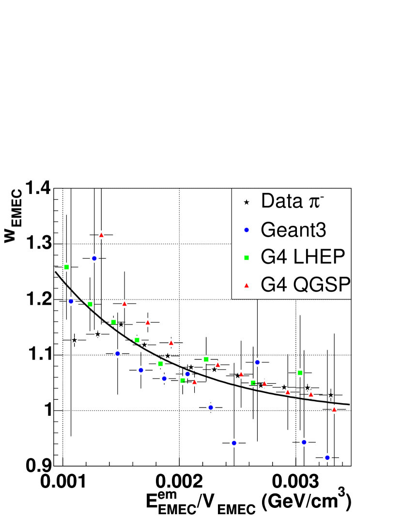
Figure 41: EMEC: Ratio (’hadronic weight’) of the true energy over the energy measured on the electromagnetic scale as function of the cluster energy density for pions of $200\,\mathrm{GeV}$. The line shows the result of the fit to the data (see text). The data are compared with MC predictions.

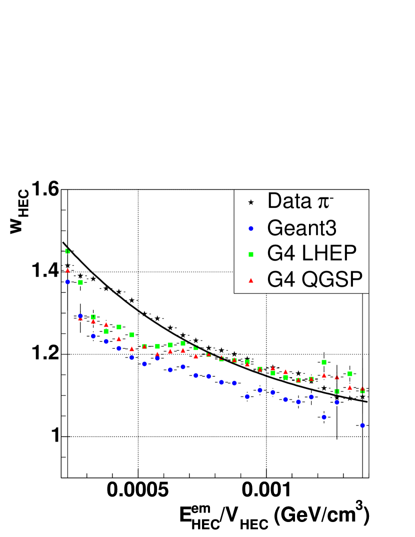
Figure 42: HEC: Ratio (’hadronic weight’) of the true energy over the energy measured on the electromagnetic scale as function of the cluster energy density for pions of $200\,\mathrm{GeV}$. The line shows the result of the fit to the data (see text). The data are compared with MC predictions.

The line shows the result of the fit to the data using the parameterisation given above 3. The corresponding fits to the MC data have been also performed. Because of the rather strong correlation between $C_{1}$ and $C_{2}$, $C_{2}$ has been set to a constant value ($C_{2}=1000\,\mathrm{cm}^{3}/\mathrm{GeV}$ for EMEC and $C_{2}=1500\,\mathrm{cm}^{3}/\mathrm{GeV}$ for HEC). It turned out that leaving $C_{2}$ as free parameter hardly improved the $\chi^{2}$ of the fit. In the EMEC the energy densities are well described by both GEANT 4 options, in contrast to GEANT 3; in the HEC the GEANT 4 models are close to the data, but far from being optimal. The two GEANT 4 models QGSP and LHEP describe the energy densities equally well, but GEANT 3 is substantially worse. The parameterisation mentioned above describes the EMEC as well as the HEC weights for the individual data sets over a large fraction of energy densities rather well.

The energy variation of the fitted parameters $C_{1}$ and $C_{3}$ for the EMEC and the HEC are shown in Figs. 43 and 44.

Figure 43: Energy dependence of the weighting parameter $C_{1}^{\rm EMEC}$ and $C_{3}^{\rm EMEC}$ for the data as function of energy.

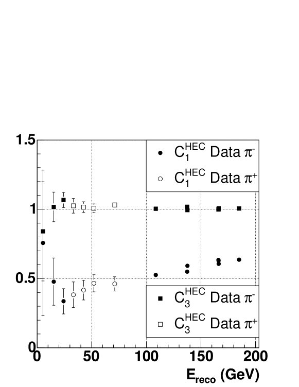
Figure 44: Energy dependence of the weighting parameters $C_{1}^{\rm HEC}$ and $C_{3}^{\rm HEC}$for the data as function of energy.

The energy dependence of all parameters shows no dramatic variation, so a parameterization of the energy dependence could easily be implemented. As expected $C_{3}$ approaches unity as given by the electromagnetic scale. Deviations from 1 are due to residual correlations with $C_{1}$, systematic errors in the determination of the electromagnetic scale or due to systematic errors in signal reconstruction, calibration and HV-correction. As seen in the data these contributions are rather small, both for the EMEC and the HEC. In ATLAS the in situ determination of $C_{3}$ with single particles can yield a powerful crosscheck not only of the electromagnetic scale of the EMEC, which is well defined from analysing e.g. ${\rm Z}\rightarrow{\rm e}^{+}{\rm e}^{-}$ decays, but also the more difficult to determine electromagnetic scale of the HEC.

Some care has to be taken when comparing the $C_{i}$’s of the data with MC predictions. The correlations between the individual parameters can result in rather different energy dependencies, yielding nevertheless a similar energy dependence of the weights. Therefore for the MC not only $C_{2}$ has been kept identical to the data (and fixed, see above), but also $C_{3}$ has been set to the value obtained from the fit to the data. In consequence, $C_{1}$ will reflect fully any deviation of the MC from the data, up to a very weak residual correlation of $C_{1}^{\rm EMEC}$ and $C_{1}^{\rm HEC}$. This approach has been chosen only to reveal clearly any differences between data and the various MC models. Figs. 45 and 46 show the results for $C_{1}^{\rm EMEC}$ and $C_{1}^{\rm HEC}$. Only $\pi^{-}$ interactions have been simulated in the MC. All MC models follow the general trend of the data, but the differences are significant. The GEANT 3 predictions deviate strongly from the HEC data and for the EMEC data none of the MC models can be preferred.

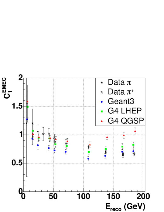
Figure 45: Energy dependence of the weighting parameter $C_{1}^{\rm EMEC}$ for the data and the different MC predictions. To optimally reveal any differences between data and MC, $C_{3}^{\rm EMEC}$ has been set in the MC to the corresponding value obtained for the data.

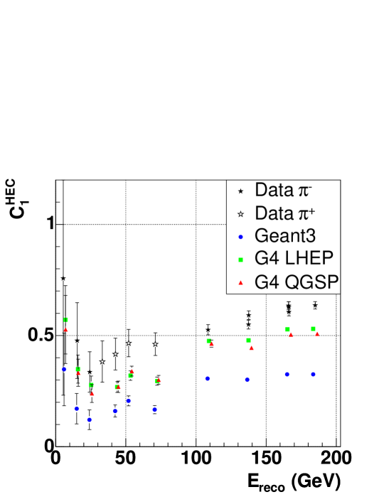
Figure 46: Energy dependence of the weighting parameter $C_{1}^{\rm HEC}$ for the data and the different MC predictions. To optimally reveal any differences between data and MC, $C_{3}^{\rm HEC}$ has been set in the MC to the corresponding value obtained for the data.

6.3 Energy Resolution using the Cluster Weighting Approach

The energy dependence of the energy resolution has been obtained using the weighting approach discussed above. The results are shown in Fig. 47 for $\pi$ data after noise subtraction. The contribution due to electronic noise is shown explicitly.

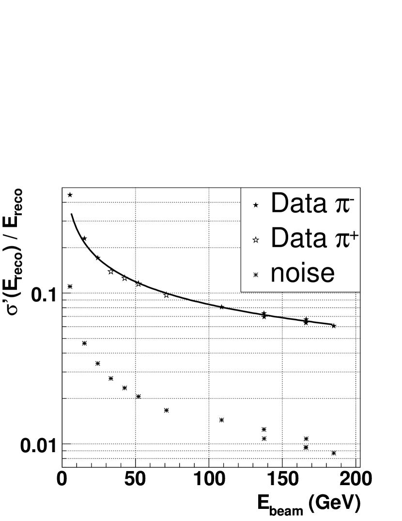
Figure 47: Energy dependence of the energy resolution for pion data using the cluster weighting approach. The noise has been subtracted, but it is shown explicitly. The line shows the result of the fit to the data.

A fit to the data with $\frac{\sigma(E)}{E}=\frac{a}{\sqrt{E}}\oplus b$ yields for the sampling term $(84.1\pm 0.3)\,$%$\sqrt{\mathrm{GeV}}$ and for the constant term zero within errors. Clearly the energy range available is not big enough to avoid any correlation between the sampling and constant term. Nevertheless, the reduction of the constant term, after the correction for leakage, gives some indication of the effectiveness of the weighting approach in achieving a good level of compensation. The direct comparison with the resolution obtained on the electromagnetic scale is shown in Fig. 48. The improvement when using the cluster weighting approach is clearly visible. The lines show the results of the fits to the data.

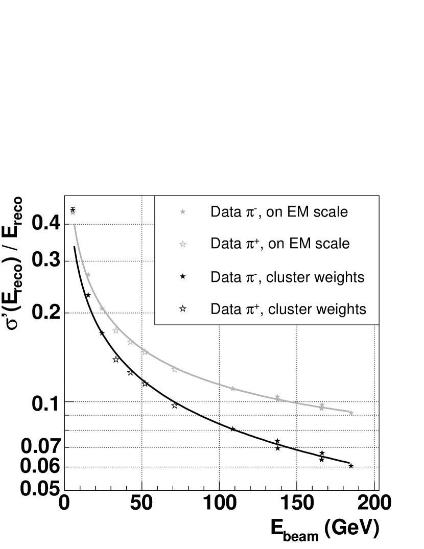
Figure 48: Energy dependence of the energy resolution for $\pi$ data using the cluster weighting approach and the corresponding results using the electromagnetic scale only. The contribution due to the electronic noise has been subtracted. The lines show the results of the fits to the data, discussed in the text.

Finally the data have been compared with MC predictions. Fig. 49 shows the energy dependence of the energy resolution, where the line shows the result of the fit to the data.

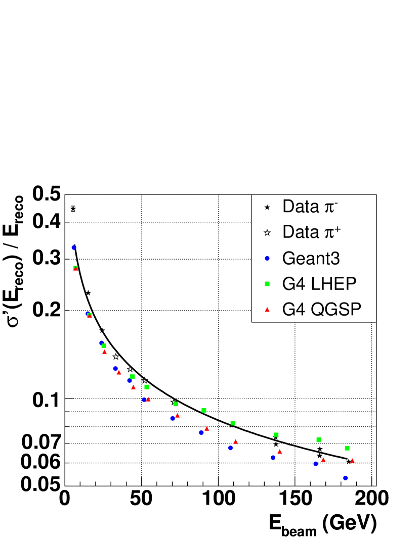
Figure 49: Energy dependence of the energy resolution for $\pi$ data using the cluster weighting approach in comparison to the different MC predictions. The contribution due to the electronic noise has been subtracted. The line shows the result of the fit to the data.

The GEANT 3 simulation predicts a sampling term of $(73.3\pm 0.5)\,$%$\sqrt{\mathrm{GeV}}$ and a vanishing constant term within errors. The GEANT 4 LHEP and QGSP simulations predict a sampling term of $(74.0\pm 0.5)\,$%$\sqrt{\mathrm{GeV}}$ and $(72.3\pm 0.9)\,$%$\sqrt{\mathrm{GeV}}$, respectively. In general, the GEANT 4 models are closer to the data, but neither QGSP nor LHEP give an optimal description. The different energy dependence of the GEANT 4 predictions is also reflected in non-vanishing constant terms: $(4.1\pm 0.1)\,$% for LHEP and $(2.5\pm 0.3)\,$% for QGSP. It has been verified that this does not result from the method of fixing the parameters $C_{2}$ and $C_{3}$ to the data values: the results for both, the constant term and the sampling term, are almost unchanged when all parameters $C_{i}$ are obtained from the fit to the MC data.

6.4 ${\rm e}/\pi$-Ratio

Using the weighting scheme an ’effective’ ${\rm e}/\pi$-ratio, the ratio between the electron and pion response, for the combined set-up EMEC/HEC can be extracted. Fig. 50 shows this ratio for the data and for the different MC models.

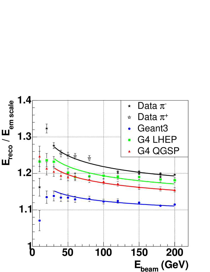
Figure 50: ${\rm e}/\pi$-ratio as obtained from the cluster weighting function. Shown is the energy dependence for the data as well as for the different MC models. The lines show the results of fits to the energy dependence.

The energy dependence is in all cases rather similar. However the MC predictions are substantially below the data, with GEANT 3 being especially low. From the energy dependence of the electromagnetic component of the hadronic shower an ${\rm e}/{\rm h}$-ratio can be obtained [3, 20, 21]. The results are using the parameterization [21] ${\rm e}/{\rm h}=1.56\pm 0.01$ for the data and ${\rm e}/{\rm h}=1.28\pm 0.01$ for GEANT 3, ${\rm e}/{\rm h}=1.48\pm 0.01$ for GEANT 4 LHEP and ${\rm e}/{\rm h}=1.42\pm 0.01$ for GEANT 4 QGSP. The errors are purely statistical. With the energy dependence being rather similar in all cases, the ’intrinsic ${\rm e}/{\rm h}$-ratio’ reflects closely the discrepancy seen already in the ${\rm e}/\pi$-ratio. However the ’intrinsic ${\rm e}/{\rm h}$-ratio’ for the combined beam test set-up has no direct interpretation for this composite calorimeter in contrast to the previous HEC stand alone set-up.

6.5 Energy Reconstruction using the Read-out Cell Weighting Approach

The energy weighting approach on the cluster level described above yields acceptable results for the case of single particles in beam tests. However in ATLAS the hadronic calibration requires the calibration of the calorimeter based on jet interactions. Here the heavy overlap of many particles dramatically reduces the power of distinction between hadronic and electromagnetic energy deposits based on cluster energy density criteria. Therefore for ATLAS a weighting approach based on the read-out cell level is envisaged [12]. The optimal procedure would be to obtain these weights from MC simulation, where on the read-out cell level the energy deposits in active and passive material are known. Lacking the MC instruments (presently in development) an approach using the data only has been tried. The basic idea is to obtain weights for individual bins of energy densities $\rho_{i}$ in the EMEC and HEC by minimizing:

$$\chi^{2}=\sum_{\rm events}{\frac{\left[E_{\rm beam}-E_{\rm leak}-E_{\rm HEC}^{\rm reco}-E_{\rm EMEC}^{\rm reco}\right]^{2}}{\left(\sigma_{\rm noise}^{\rm em}\right)^{2}+\left(\sigma_{\rm noise}^{\rm leak}\right)^{2}}},$$

with

$$E_{\rm EMEC/HEC}^{\rm reco}=\sum_{i=1}^{N}{\left[w_{\rm EMEC/HEC}^{i}\!\!\!\!\!\!\sum_{{\rm cells~{}with}~{}\rho_{i}\leq\rho_{\rm cell}\leq\rho_{i+1}}{\!\!\!\!\!E_{\rm cell}^{\rm em}}\right]}.$$

An important aspect is to correct for the energy leakage prior to minimizing the $\chi^{2}$, because the energy leakage can affect $\chi^{2}$ more than any difference in the electron to pion response of the calorimeter. The number of parameters determined in the fit was typically $N=26$ for EMEC and $N=26$ for the HEC (25 bins in each energy weighting histogram, plus one overflow bin). Figs. 51 and 52 show the results obtained for the weights $w_{i}$ for the EMEC and HEC for pions of $200\,\mathrm{GeV}$.

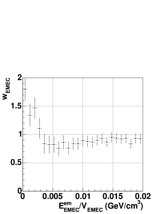
Figure 51: Read-out cell weighting approach: weights obtained for the EMEC for pions of $200\,\mathrm{GeV}$.

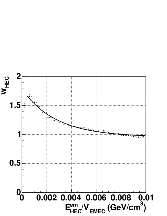
Figure 52: Read-out cell weighting approach: weights obtained for the HEC for pions of $200\,\mathrm{GeV}$. The line shows the result of the fit.

Again, a parameterization of the type

$$w\left(\frac{E_{\rm cell}^{\rm em}}{V_{\rm cell}}\right)=C_{1}\exp\left(-C_{2}\frac{E_{\rm cell}^{\rm em}}{V_{\rm cell}}\right)+C_{3}$$

yields at least for the HEC a good parameterization (see Fig. 52).

The method to extract the weights directly from the data rather than using the MC has a drawback: the weights obtained from the fit are to some extent correlated and reflect more than the pure e to $\pi$ compensation. Fig. 53 shows the correlation coefficients between the individual weights for the $2$ sets of $26$ weights obtained from the fit for pions of $200\,\mathrm{GeV}$.

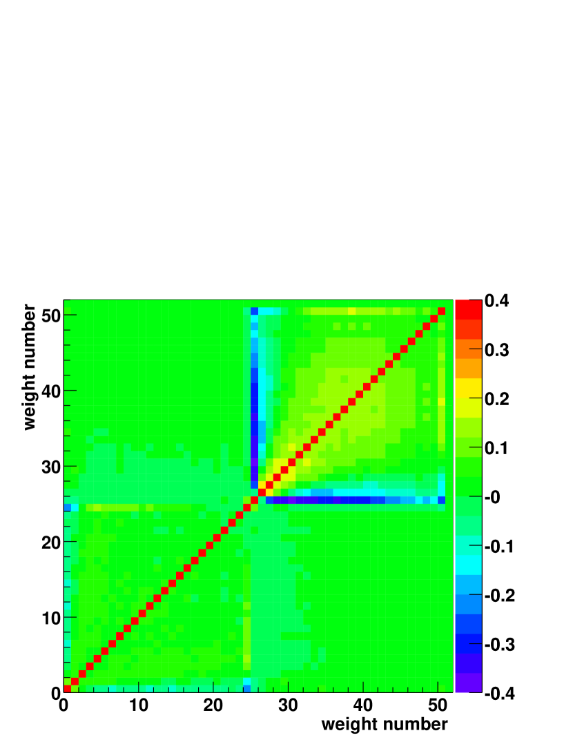
Figure 53: Correlation coefficients between the individual weights for the $2$ sets of $26$ weights ($26$ weights for the EMEC, $26$ weights for the HEC) obtained from the fit for pions of $200\,\mathrm{GeV}$. The axes run over weight numbers ($0$-$25$ for the EMEC and $26$-$51$ for the HEC).

The two sets of EMEC and HEC weights are uncorrelated. But there is a sizeable anti-correlation between the weights for low densities and all other energy densities for the individual EMEC and HEC sets of weights. The sensitivity of this method to even very small imperfections is a severe limitation. This can be demonstrated nicely by applying the method to electrons. Fig. 54 shows the weights obtained in this case for electrons of $148\,\mathrm{GeV}$.

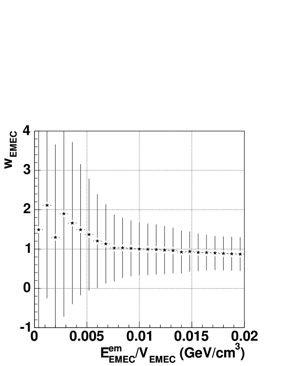
Figure 54: Weights obtained from the read-out cell weighting approach applied to electrons of $148\,\mathrm{GeV}$. Shown is the dependence on the energy density in the EMEC.

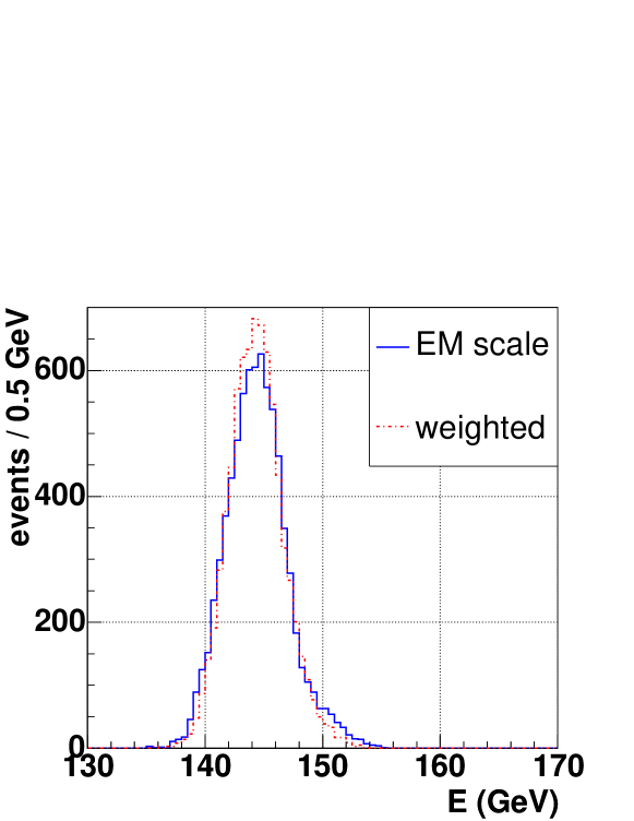
Figure 55: Read-out cell weighting approach applied to electrons of $148\,\mathrm{GeV}$. Shown is the energy distribution using the standard electromagnetic scale (solid histogram) and the result using the read-out cell weights (dashed histogram) determined for electrons.

Again, the weights at low energy densities deviate from the nominal electromagnetic scale, and are anti-correlated with the corresponding weights at high energy densities. Fig. 55 shows the energy distribution for electrons of $148\,\mathrm{GeV}$ using the nominal electromagnetic scale (solid histogram) and the cell weights (dashed histogram). The actual energy distribution is hardly changed at all. The correlation coefficients for the cell weights are shown in Fig. 56.

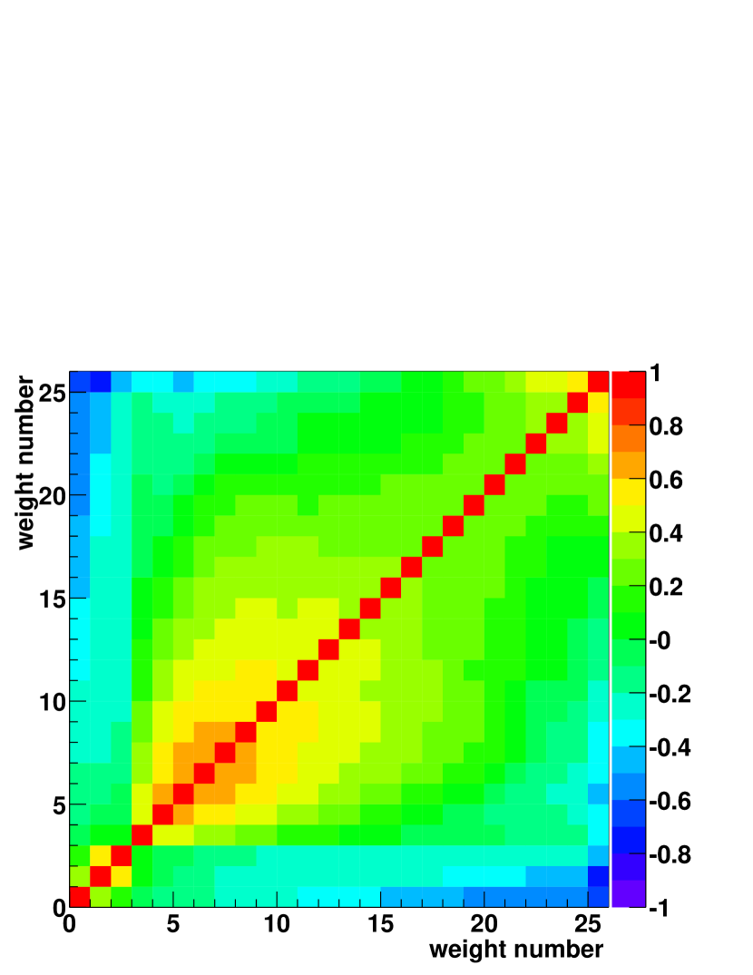
Figure 56: Read-out cell weighting approach applied to electrons of $148\,\mathrm{GeV}$. Shown are the correlation coefficients between the EMEC weights obtained. The axes run over weight numbers ($0$-$25$ for the EMEC).

6.6 Energy Resolution using the Read-out Cell Weighting Approach

The energy resolution for pions has been determined using the read-out cell weighting approach. Fig. 57 shows the energy dependence of the energy resolution obtained. The electronic noise contribution has been again subtracted, but is shown explicitly.

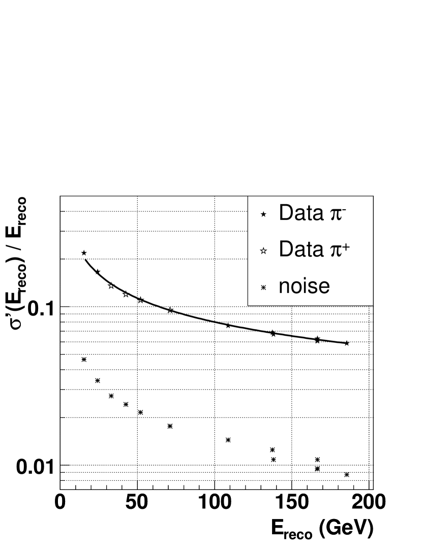
Figure 57: Read-out cell weighting approach: Energy dependence of the energy resolution for pions. The electronic noise has been subtracted, but is shown explicitly.

Using the parameterisation $\frac{\sigma(E)}{E}=\frac{a}{\sqrt{E}}\oplus b$ a sampling term of $(80.1\pm 0.3)\,$%$\sqrt{\mathrm{GeV}}$ is obtained. The constant term is compatible with being zero. This result is very close to the result obtained using the cluster weighting approach.

6.7 Impact of Hadronic Weights on Energy of Electromagnetic Clusters

In the weighting approach for the hadronic calibration it has to be guaranteed that even clusters with almost pure electromagnetic energy are reconstructed at the correct energy scale. To test this, electrons have been reconstructed using the hadronic weights. Figs. 58 and 59 show the energy distributions for electrons of $100\,\mathrm{GeV}$ using the cluster weighting and read-out cell weighting approach (weights defined from pions, dashed histogram) respectively compared to the normal (electromagnetic scale, solid histogram) reconstruction.

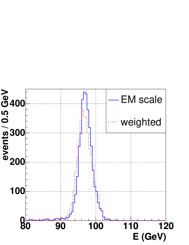
Figure 58: Energy distribution of electrons of $100\,\mathrm{GeV}$ using the cluster weighting approach (dashed histogram) with pion weights in comparison with the energy reconstruction using the electromagnetic scale (solid histogram).

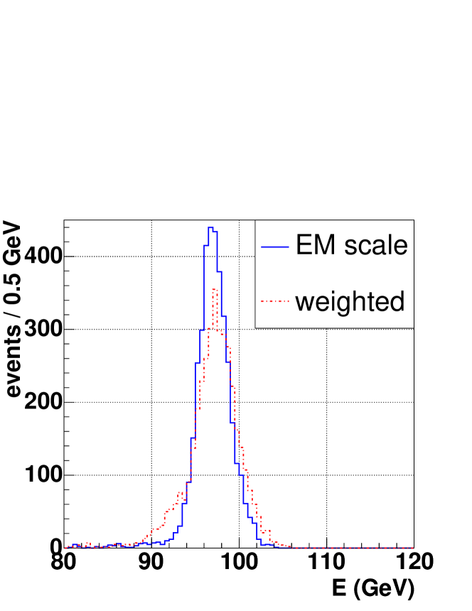
Figure 59: Energy distribution of electrons of $100\,\mathrm{GeV}$ using the read-out cell weighting approach (dashed histogram) with pion weights in comparison with the energy reconstruction using the electromagnetic scale (solid histogram).

In both cases the mean energy is obtained correctly, but the resolution is deteriorated. The requirement, not to distort the electromagnetic energy scale, is important for any weighting approach to be applied to clusters in the ATLAS calorimeter. Therefore any algorithm developed to compensate for the different ${\rm e}/\pi$ response in the ATLAS calorimeter has to fulfill this requirement.

7 Conclusions

Results of calibration runs with electrons and pions in the ATLAS end-cap calorimeter corresponding to the region in pseudorapidity around $|\eta|=1.6$-$1.8$ in ATLAS have been presented. The electromagnetic calibration constants have been determined for both subdetectors, the EMEC as well as the HEC. First steps of the ATLAS hadronic calibration strategy have been tested. The signal weighting approach, as used in previous experiments, improves the pion energy resolution substantially: using the ansatz $\frac{\sigma(E)}{E}=\frac{a}{\sqrt{E}}\oplus b$ a sampling term of typically $a\approx 80\,$%$\sqrt{\mathrm{GeV}}$ can be achieved and a vanishing constant term $b$. For ATLAS the hadronic calibration has to deal with jets rather than single particles. Therefore the transfer of weighting constants from the beam test to ATLAS is only possible when using MC simulation. One of the important steps in this procedure is to validate the MC via comparison of the simulation results with pion data. This has been initiated in detail using GEANT 3 and GEANT 4 simulations. In general GEANT 4 yields the better description of the data, but not yet at the level required. Whereas the agreement of the GEANT 4 prediction with data for the response at the electromagnetic scale is rather good, GEANT 4 fails to describe the details of hadronic shower fluctuations at the level required to apply weighting techniques. Here further improvements of GEANT 4 parameters and processes are required.

References

- [1] B. Aubert et al., Performance of the ATLAS electromagnetic end-cap module 0, Nucl. Instr. and Meth. A500 (2003) 178.
- [2] B. Aubert et al., Performance of the ATLAS electromagnetic barrel module 0, Nucl. Instr. and Meth. A500 (2003) 202.
- [3] B. Dowler et al., Performance of the ATLAS Hadronic End-Cap Calorimeter in Beam Tests, Nucl. Instr. and Meth. A482 (2002) 94.
- [4] H. Bartko, Performance of the Combined ATLAS Liquid Argon End-Cap Calorimeter in Beam Tests at the CERN SPS, Diploma Thesis, Technical University Munich, 2003, ATLAS-COM-LARG-2004-004.
-
[5]
S. Simion, Liquid Argon Calorimeter ROD, 2nd ATLAS ROD workshop, October 2000,
University of Geneva,
. - [6] W.E. Cleland, E.G. Stern, Signal processing consideration for liquid ionization calorimeters in a high rate environment, Nucl. Instr. and Meth. A338 (1994) 467-497.
- [7] L. Kurchaninov, P.Strizenec, Calibration and Ionization Signals in the Hadronic End-Cap Calorimeter of ATLAS, IX International Conference on Calorimetry in High Energy Physics, Annecy, France, 9-14 October, 2000, Frascati Physics Series Vol. XXI, 219-226, 2000.
- [8] L. Neukermans, P. Perrodo and R. Zitoun, Understanding the ATLAS electromagnetic barrel pulse shapes and the absolute electronic calibration, ATL-LARG-2001-008.
- [9] Marco Delmastro, Energy Reconstruction and Calibration Algorithms for the ATLAS Electromagnetic Calorimeter, PhD thesis, Universita Degli Studi di Milano, 2002, .
- [10] M. Vincter, C. Cojocaru, Electronic Noise in the 2002 HEC/EMEC Testbeam, ATLAS-HEC-Note-149 (2003).
- [11] M. Lefebvre and D. O’Neil, Endcap Hadronic Calorimeter Offline Testbeam Software, ATLAS-LARG-99-002, January 1999.
-
[12]
C. Alexa et al., Hadronic Calibration of the ATLAS Calorimeter, 2003,
. - [13] R. Brun et al., GEANT 3, CERN DD/EE/84-1, 1986.
- [14] A. Kiryunin and D. Salihagic, Monte Carlo for the HEC Prototype: Software and Examples of Analysis, ATLAS HEC Note-063 (1998).
- [15] C.Zeitnitz and T.A. Gabriel, The GEANT-CALOR interface and benchmark calculations of ZEUS test calorimeters, Nucl. Instr. and Meth. A349 (1994) 106.
- [16] S. Agostinelli et al., GEANT 4 - a simulation toolkit, Nucl. Instr. and Meth. A506 (2003) 250.
-
[17]
J.P. Wellisch,
. - [18] I. Abt et al., The tracking, calorimeter and muon detectors of the H1 experiment at HERA, Nucl. Instr. and Meth. A386 (1997) 348.
- [19] B. Andrieu et al., Results from pion calibration runs for the H1 liquid argon calorimeter and comparisons with simulations, Nucl. Instr. and Meth. A336 (1993) 499.
- [20] R. Wigmans, High resolution hadronic calorimetry, Nucl. Instr. and Meth. A265 (1988) 273.
- [21] D. Groom, What really goes on in a hadronic calorimeter, VII International Conference on Calorimetry in High Energy Physics, Tuscon, Arizona, November 9-14, 1997.