Optimization and performance of an optical cardio-magnetometer

Abstract

Cardiomagnetometry is a growing field of noninvasive medical diagnostics that has triggered a need for affordable high-sensitivity magnetometers. Optical pumping magnetometers are promising candidates satisfying that need since it was demonstrated that thy can map the heart magnetic field. For the optimization of such devices theoretical limits on the performance as well as an experimental approach is presented. The promising result is a intrinsic magnetometric sensitivity of 63 fT$/\sqrt{\mathrm{Hz}}$ a measurement bandwidth of 140 Hz and a spatial resolution of 28 mm.

I Introduction

Biomagnetometry is a rapidly growing field of noninvasive medical diagnostics andrae . In particular, the magnetic fields generated by the human heart and brain carry valuable information about the underlying electrophysiological processes wikswo . Since the 1970s superconducting quantum interference devices (SQUIDs) have been used to detect these generally very weak biomagnetic fields cohen . The magnetic field of the human heart is the strongest biomagnetic signal, with a peak amplitude of 100 $\mathrm{pT}$, but since this is still orders of magnitude weaker than typical stray field interference the measurement of such signals could initially only be performed inside expensive magnetically-shielded rooms (MSR). Progress in medical research in the past decade has motivated a need for more affordable cardiomagnetic sensors. Recently, multichannel SQUIDs were developed that no longer require shielding due to the use of gradiometric configurations. Such devices are commercially available but are still quite expensive in both capital and operational costs.

Optical pumping magnetometers (OPM) have been widely known since the 1960s bloom , and offer both high sensitivity and reliable operation for research cohen-tann and applications like geomagnetometry alexandrov3decades . Since OPMs usually work with a near room-temperature thermal alkali metal vapor, they avoid the need for the cryogenic cooling that makes SQUIDs so costly and maintenance intensive. Our goal was to develop an affordable, maintenance-free device that is both sensitive and fast enough to measure the magnetic field of the human heart. In order to be competitive with the well-established SQUIDs, a cardiomagnetic sensor has to offer a magnetic field sensitivity of at least 1 $\mathrm{pT}$ with a bandwidth of about 100 $\mathrm{Hz}$. Furthermore, the spatial resolution of the sensor has to be better than 4 $\mathrm{cm}$, the standard separation of grid points during mapping.

Since the cardiomagnetometry community is mainly interested in one of the components of the magnetic field vector, one might think of using vector-type OPMs like the Hanle magnetometer kastlerhe or the Faraday magnetometer, devices which operate in zero fields only budker_pra_2000 . However, these devices lose their sensitivity in the presence of even tiny field components in directions perpendicular to the field of interest. The broadening caused by such transverse field components must be kept well below the width of the magnetometer resonance budker_pra_2000 , thus limiting those components to values below a few tenths of $\mathrm{pT}$. Accordingly, optical vector magnetometers cannot be used for cardiomagnetometry in a straightforward way since the heart field features time-varying transverse field components on the order of 100 $\mathrm{pT}$. We have therefore concentrated on the $M_{x}$ OPM, which exhibits a fast response and which has been shown to be sufficiently sensitive in an unshielded environment. Furthermore, lamp-pumped $M_{x}$ OPMs were used for the first biomagnetic measurements kozlov1 with optical magnetometers in the early 1980s, although that work was discontinued. Instead of lamps, we use diode lasers as a light source in order to build a device that will scale to the many channels needed for fast mapping of the cardiomagnetic field.

II Principle of scalar OPM operation

Optically pumped magnetometers operate on the principle that the optical properties of a suitable atomic medium are coupled to its magnetic properties via the atomic spin. The ensemble average of the magnetic moments associated with the spins can be treated as a classical magnetization vector $\mathbf{M}=N_{F}g_{F}\,\mu_{B}\langle\mathbf{F}\rangle/\hbar$ in space. Here $N_{F}\langle\mathbf{F}\rangle=N_{F}\,\mathrm{tr}(\rho_{F}\mathbf{F})$ with $\mathrm{tr}\,\rho_{F}=1$ is the total angular momentum of $N_{F}$ atoms in an optical hyperfine level $F$ where $\rho_{F}$ is the density matrix and $g_{F}$ the Landé factor of the state. Optical magnetometers detect changes of the medium’s optical properties induced by the precession of $\mathbf{M}$ in a magnetic field $\mathbf{B}_{\mathrm{tot}}$. The frequency of this precession, the Larmor frequency $\omega_{L}$, is proportional to the modulus of $\mathbf{B}_{\mathrm{tot}}$:

$$\omega_{L}=\frac{g_{F}\mu_{B}}{\hbar}\left|\mathbf{B}_{\mathrm{tot}}\right|\quad\equiv\quad\gamma_{F}\left|\mathbf{B}_{\mathrm{tot}}\right|.$$ (1)

For Cs the constant of proportionality, $\gamma_{F}$, has a value of $2\pi\times 3.5\>\mathrm{Hz}/\mathrm{nT}$. All atomic vapor magnetometers measure the magnetic field via a direct or indirect measurement of the Larmor frequency.

II.1 The $M_{x}$ magnetometer

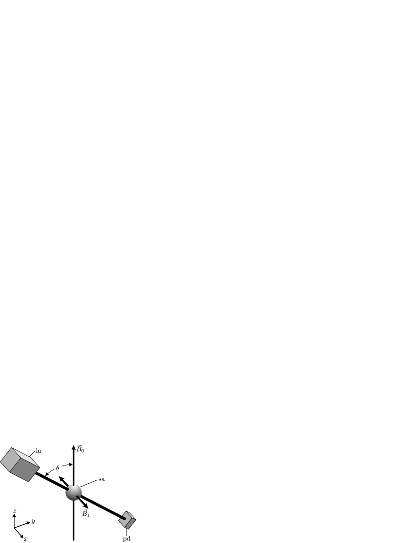
Figure 1: Basic geometry of the $M_{x}$-magnetometer setup: The laser (la) emits a beam that traverses the sample (sa) at angle $\theta$ with respect to the magnetic field $\mathbf{B}_{0}$. The transmitted power is detected by a photodetector (pd). The static magnetic field $\mathbf{B}_{0}$ is aligned along the $z$-direction. The oscillating magnetic field $\mathbf{B}_{1}$ is aligned along the $x$-direction.

In the case of the $M_{x}$ magnetometer, a magnetic-resonance technique is used to measure the Larmor frequency directly, by employing two perpendicular magnetic fields $\mathbf{B}_{0}$ and $\mathbf{B}_{1}$. The static magnetic field $\mathbf{B}_{0}$ is aligned along the $z$-direction. As Fig. 1 shows, the $\mathbf{k}$-vector of the laser beam lies in the $yz$-plane and is oriented at an angle $\theta$ with respect to the $z$-direction. The magnetometer is sensitive to the modulus of $\mathbf{B}_{0}$. The oscillating magnetic field $\mathbf{B}_{1}=\hat{x}B_{\mathrm{rf}}\cos\omega_{\mathrm{rf}}t$ is aligned along the $x$-direction with an amplitude much smaller than $B_{0}$.

In order to introduce the basic concepts we discuss the simplest case of an $F=1/2$ state. The motion of $\mathbf{M}$ under the influence of $\mathbf{B}_{0}$ and $\mathbf{B}_{1}$ is then given by the Bloch equations:

$$\left(\begin{array}[]{c}\dot{M}_{x}\\ \dot{M}_{y}\\ \dot{M}_{z}\end{array}\right) = \left(\begin{array}[]{c}M_{x}\\ M_{y}\\ M_{z}\end{array}\right)\times\left(\begin{array}[]{c}\gamma_{F}B_{\mathrm{rf}}2\cos\omega_{\mathrm{rf}}t\\ 0\\ \gamma_{F}B_{0}\end{array}\right)$$ (18)

$${}-\left(\begin{array}[]{c}\gamma_{2}M_{x}\\ \gamma_{2}M_{y}\\ \gamma_{1}M_{z}\end{array}\right)+\Gamma_{P}\left(\begin{array}[]{c}\phantom{-M_{0}\sin\theta}-M_{x}\\ \phantom{-}M_{0}\sin\theta-M_{y}\\ -M_{0}\cos\theta-M_{z}\end{array}\right)\>.$$

The first term describes the precession of $\mathbf{M}$ around the magnetic fields. The second term describes the longitudinal ($\gamma_{1}$) and transverse ($\gamma_{2}$) relaxation of $\mathbf{M}$. The third term represents the effect of optical pumping with circularly polarized light that creates the magnetization. It can be treated as an additional relaxation leading to an equilibrium orientation aligned with the $\mathbf{k}$-vector of the incoming light at the pumping rate $\Gamma_{P}$. Both relaxations add up to the effective relaxation rates $\Gamma_{1,2}=\gamma_{1,2}+\Gamma_{P}$. In the case of small $B_{\mathrm{rf}}$ amplitudes, Eq. (18) can be solved using the rotating–wave approximation millihertz which leads to a steady-state solution where $\mathbf{M}$ rotates around $\mathbf{B}_{0}$ at the driving frequency $\omega_{\mathrm{rf}}$.

The optical property used in the $M_{x}$ magnetometer is the optical absorption coefficient which determines the power, $P$, of the light transmitted through the medium. For circularly polarized light, the transmitted power is proportional to the projection of $\mathbf{M}$ on the $\mathbf{k}$-vector of the incoming light. Therefore, the precessing magnetization results in a modulation of the absorption index measurable as an oscillation of $P$. The in-phase and quadrature components of $P$ with respect to the driving field can be obtained from Eq. (18):

$$P_{\mathrm{ip}}(\delta) = -P_{0}\sin(2\theta)\frac{\Omega_{\mathrm{rf}}\delta}{\Omega_{\mathrm{rf}}^{2}\Gamma_{2}/\Gamma_{1}+\Gamma_{2}^{2}+\delta^{2}}\>\mbox{, and}$$ (19)

$$P_{\mathrm{qu}}(\delta) = -P_{0}\sin(2\theta)\frac{\Omega_{\mathrm{rf}}\Gamma_{2}}{\Omega_{\mathrm{rf}}^{2}\Gamma_{2}/\Gamma_{1}+\Gamma_{2}^{2}+\delta^{2}}\>.$$ (20)

Here $\Omega_{\mathrm{rf}}=\gamma_{F}B_{\mathrm{rf}}$ is the Rabi frequency and $\delta=\omega_{\mathrm{rf}}-\omega_{L}$ the detuning of the oscillating field $\mathbf{B}_{1}$ from the Larmor frequency. The constant $P_{0}$ combines all factors such as the initial light power, the number of atoms in the sample, and the cross section for light-atom interactions determining the absolute amplitude of the signal. The components can be measured using phase-sensitive detection. The signals are strongest for $\theta=45^{\circ}$, which was used in all experiments.

Figure 2: (a) Measured magnetic resonance lineshapes of the in-phase ($a_{1}$) and quadrature signals ($a_{2}$), measured in a single sweep of 20 s with the cardiomagnetometer placed in a poorly shielded room. Magnetic 50 $\mathrm{Hz}$ line interference was suppressed using a $4^{th}$ order lowpass filter (time constant 10 ms). The half-width, derived from a fit, was $\Delta\omega_{\mathrm{HW}}/2\pi=173\>\mathrm{Hz}$. (b) Magnetic resonance line shape of the oscillation phase measured with respect to the driving field $B_{\mathrm{rf}}$. The data was obtained in real time using a digital lock-in amplifier. The fitted half-width is: $\Delta\omega^{\varphi}_{\mathrm{HW}}/2\pi=109\>\mathrm{Hz}$.

Both $P_{\mathrm{ip}}$ and $P_{\mathrm{qu}}$ show resonant behavior near $\delta=0$. $P_{\mathrm{qu}}$ has an absorptive Lorentzian line shape, and $P_{\mathrm{ip}}$ has a dispersive Lorentzian line shape with the same half width expressed as

$$\Delta\omega_{\mathrm{HW}}=\sqrt{\Omega_{\mathrm{rf}}^{2}\Gamma_{2}/\Gamma_{1}+\Gamma_{2}^{2}}=\Gamma_{2}\sqrt{S+1}\,.$$ (21)

Here $S=\Omega^{2}/(\Gamma_{1}\Gamma_{2})$ is the saturation parameter of the rf field. Figure 2(a) shows measured line shapes under conditions optimized for maximal magnetometric sensitivity (see Sec. IV for details).

Signal $P_{\mathrm{ip}}$ is of particular interest because it has a dispersive shape, featuring a steep linear zero-crossing at $\delta=0$. In this region $P_{\mathrm{ip}}$ can be used to measure the deviation of $\mathbf{B}_{0}$ from the value that corresponds to $\omega_{\mathrm{rf}}$. The same is true for the deviation of the phase difference $\varphi$ between the measured oscillation and the driving field from -90^∘ (see Fig. 2(b)). The phase difference $\varphi$ can be calculated from $P_{\mathrm{ip}}$ and $P_{\mathrm{qu}}$, yielding

$$\tan\varphi=\frac{P_{\mathrm{qu}}}{P_{\mathrm{ip}}}=\frac{\Gamma_{2}}{\delta}\>.$$ (22)

The phase signal changes from $\varphi=0$ at low frequencies to $\varphi=-\pi$ at high frequencies. For practical reasons it is preferable to shift the phase by 90^∘ so that it passes through zero in the center of the resonance ($\delta=0$). This can easily be done by shifting the reference signal by $\pi/2$ using the corresponding feature of the phase detector. In mathematical terms that 90^∘ shift is equivalent to the transformation $P_{\mathrm{qu}}\rightarrow-P_{\mathrm{ip}}$ and $P_{\mathrm{ip}}\rightarrow P_{\mathrm{qu}}$, yielding

$$\tan\varphi^{\prime}=-\frac{\delta}{\Gamma_{2}}.$$ (23)

The width of the phase signal $\Delta\omega^{\varphi}_{\mathrm{HW}}$ is smaller than $\Delta\omega_{\mathrm{HW}}$ because it is not affected by rf power broadening, i.e., it is independent of $\Omega_{\mathrm{rf}}$:

$$\Delta\omega^{\varphi}_{\mathrm{HW}}=\Gamma_{2}<\Delta\omega_{\mathrm{HW}}\>.$$ (24)

The narrower lineshape of the phase signal is exactly compensated by a better S/N ratio of $P_{\mathrm{ip}}$  [see Eqs. (21), (26), and (27)] resulting in a statistically equivalent magnetic field resolution for both signals. However, since the lineshape of the phase signal depends only on $\Gamma_{2}$, it is easier to calibrate in absolute field units. Furthermore, light amplitude noise, for instance caused by fluctuating laser intensities, does not directly affect the phase signal, since both $P_{\mathrm{ip}}$ and $P_{\mathrm{qu}}$ scale in the same way with light intensity. Only the much weaker coupling via the light shift can cause the phase signal to reflect light amplitude noise. Considering those practical advantages of the phase signal we concentrate in the following sections on the sensitivity of the phase signal to magnetic field changes.

II.2 Nyquist plots

Figure 3: Nyquist plots for three different values of $S$. The solid line is for $S=1$, the dashed lines are for $S=0.25$ (nearly round) and $S=4$ (elliptical), respectively. If $\omega_{\mathrm{rf}}$ is scanned towards increasing values the system evolves clockwise through the Nyquist plot.

The lineshapes $P_{\mathrm{ip}}(\delta)$, and $P_{\mathrm{qu}}(\delta)$ of the magnetic resonance have a major influence on the magnetometric sensitivity. The magnetic resonances in Eqs. (19) and (20) can be interpreted as a complex transfer function $t(\omega)$ connecting the current that drives the rf-coils, $I_{i}=I_{0}\exp(i\omega t)+c.c.$, and the photocurrent $I_{p}=t(\omega)I_{i}$ of the photodiode. By setting the effective transverse relaxation rate $\Gamma_{2}$ as the unit of frequency and using the normalized detuning $x\;(=\delta/\Gamma_{2})$, $t$ can be written in dimensionless units as:

$$t=t_{0}\frac{\sqrt{S}(i+x)}{1+S+x^{2}}\;.$$ (25)

A parametric plot of $t(x)$ in the complex plane — called a Nyquist plot — was found to be useful for the inspection of experimental data. In this representation $t(x)$ appears as an ellipse with diameters $d_{r}$ and $d_{i}$ for the real (in-phase) and imaginary (quadrature) components respectively (see Fig. 3):

$$d_{r} = t_{0}\sqrt{\frac{S}{1+S}}$$ (26)

$$d_{i} = t_{0}\frac{\sqrt{S}}{1+S}\>.$$ (27)

The saturation parameter of the rf transition, $S$, can be extracted from the ratio of the two diameters:

$$S=\frac{\Omega^{2}}{\Gamma_{1}\Gamma_{2}}=\frac{d_{r}^{2}}{d_{i}^{2}}-1.$$ (28)

Figure 4: Nyquist plot of a resonance with $S=1$ when an interfering sine wave of amplitude $r_{i}$ and phase $\varphi_{i}$ is added. A phase offset of $\Delta\varphi$ in the demodulation due to a poorly adjusted lock-in phase leads to a rotated ellipse.

Figure 4 shows a Nyquist plot of a resonance for a situation in which an interfering sine wave is added to the photocurrent, leading to a shifted ellipse. The amplitude $r_{i}$ and the phase $\varphi_{i}$ of the interference can be easily extracted from the Nyquist plot. A phase shift in the demodulation leads to a rotated ellipse. In this situation the spectra of in-phase $P_{\mathrm{ip}}(\delta)$ and quadrature $P_{\mathrm{qu}}(\delta)$ components as a function of rf detuning appear asymmetric.

By means of Nyquist plots it is easy to distinguish between an asymmetry caused by improper adjustment of the lock-in phase and one caused by inhomogeneous broadening. The latter causes a deviation from the elliptical shape. One model for inhomogeneous broadening is to assume a gradient in the static magnetic field. Since we use buffer-gas cells the atoms do not move over large distances during their spin coherence lifetime so that inhomogeneous magnetic fields are not averaged out. Instead, atoms at different locations in the cell see different magnetic fields, resulting in an inhomogeneous broadening of the magnetic resonance line.

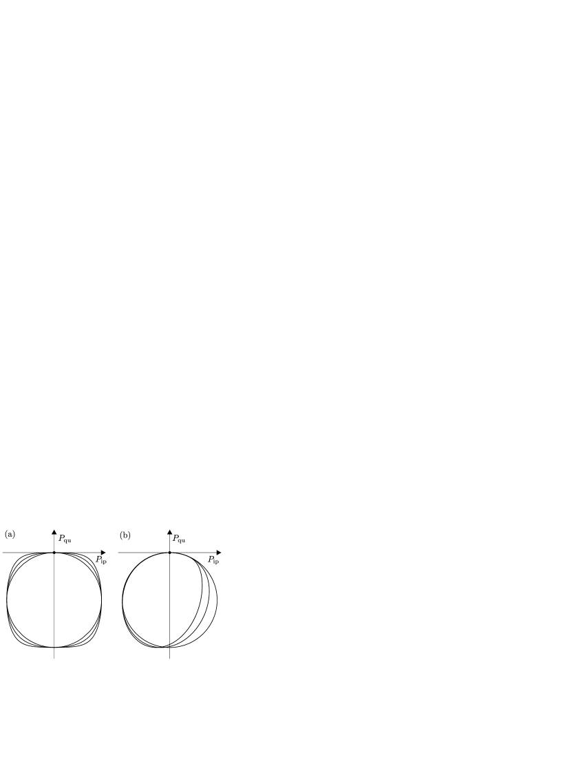
Figure 5: Nyquist plots for different magnetic field distributions, each scaled to fit in a square of length 1. Part (a) shows the deviation from circular for constant magnetic field distributions. The innermost trace is for an unperturbed resonance. The two outer traces are calculated for field distribution widths of $x_{g}=40\,\Gamma_{2}$ and $400\,\Gamma_{2}$, respectively. Part (b) shows the deviation from circular for linear field distributions. The (outer) circular trace is for an unperturbed resonance. The other two are calculated for distribution widths of $x_{g}=5\,\Gamma_{2}$ and $10\,\Gamma_{2}$, respectively.

Figure 5 shows calculated Nyquist plots for different gradients of the static field $\mathbf{B}_{0}$. The simplest model for such an inhomogeneity is a constant gradient $\mathrm{d}B_{z}/\mathrm{d}z$ over the length $l_{z}$ of the cell. This is expressed by a convolution of the theoretical magnetic resonance signals $t(x)$ [see Eq. (25)] with the normalized distribution of magnetic fields $g(x)$ which, in this case, is a constant over the interval

$$2x_{g}=\frac{\gamma_{F}}{\Gamma_{2}}l_{z}dB_{z}/dz\,.$$ (29)

Since $g(x)$ vanishes everywhere except for $-x_{g}\leq x\leq x_{g}$ the convoluted resonance $t^{\prime}$ is given by

$$t^{\prime}(x) = \int_{-{x_{g}}}^{x_{g}}\!t(x-x^{\prime})\,g(x^{\prime})\,\mathrm{d}x^{\prime}\,,$$ (30)

which can be evaluated analytically

$$t^{\prime} = \frac{\sqrt{S}}{4\,x_{g}}\left[\ln\left\{1+S+(x_{g}-x)^{2}\right\}\right.$$ (31)

$$\left.-\ln\left\{1+S+(x_{g}+x)^{2}\right\}\right]$$

$$-\,\frac{i}{2\,x_{g}}\sqrt{\frac{S}{1+S}}\left\{\arctan\left(\frac{x_{g}-x}{\sqrt{1+S}}\right)\right.$$

$$+\left.\arctan\left(\frac{x_{g}+x}{\sqrt{1+S}}\right)\right\}\,.$$

The main effect of the constant magnetic field distribution is to broaden the resonance, to decrease the amplitude, and to make the line shape differ from a Lorentzian. In the Nyquist plot this is seen by a deformation of the elliptical trace towards a rectangular trace as shown in Fig. 5(a). The effect is clearly visible in Fig. 5(a) for rather large widths of the magnetic field distribution; in the experiment, however, the effect can be detected for much smaller inhomogeneities due to the large signal/noise ratio.

III Experimental Setup

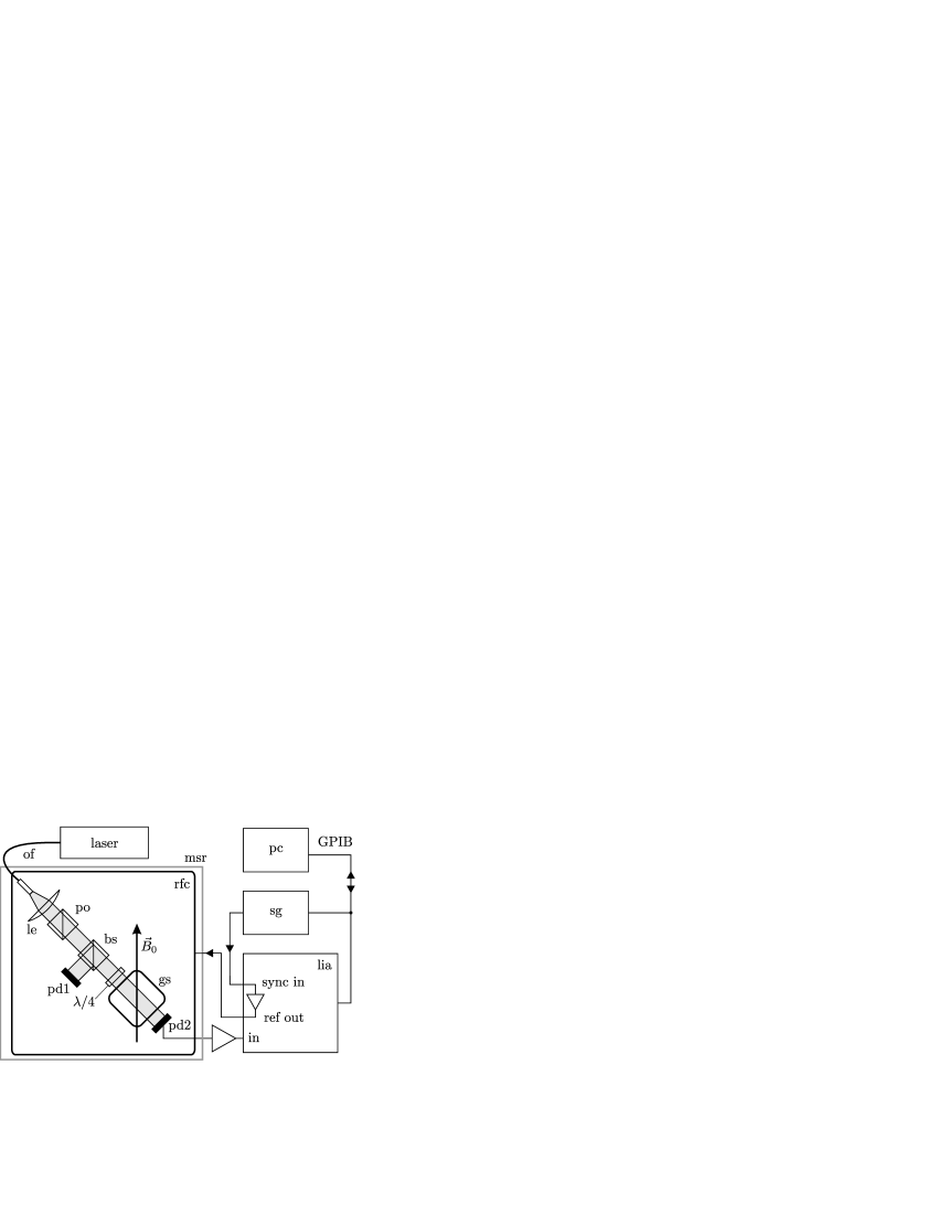
Figure 6: Schematic of the experimental setup. Light from the diode laser is delivered via an optical fiber (of) to the experiment in the magnetically shielded room (msr). The light is collimated by a lens (le) and polarized by a polarizing beam splitter cube (po). The beam splitter (bs) reflects 50% of the beam to photodiode 1 (pd1) used for monitoring of the initial light power. The remaining beam passes a quarter-wave plate ($\lambda/4$) providing circular polarized light to the glass cell (gs) that contains the atomic medium. Photodiode 2 (pd2) measures the transmitted light intensity. Its signal is amplified by a current amplifier and fed to the lock-in amplifier (lia). The reference output of the lia drives the radio frequency coils (rfc). The reference frequency of the lia is controlled by a sweep generator (sg). Automatic control and data aquisition is done by a PC via the GPIB bus.

The magnetometer described here was part of the device used by us to measure the magnetic field of the human heart bison1 ; bison2 . The setup was designed so that a volunteer could be placed under the sensor, with his heart close to the glass cell containing the Cs sample. For moving the volunteer with respect to the sensor—necessary for mapping the heart magnetic field—a bed on a low friction support was used.

The magnetometer sensor head itself was placed in a room with moderate magnetic shielding. The room was $1.7\times 2.3\times 2.5\>\mathrm{m}^{3}$ in volume shielded by a 1 mm $\mu$-metal layer and an 8 mm copper-coated aluminum layer. For low frequencies, the shielding factor was as low as 5 to 10, whereas 50 $\mathrm{Hz}$ interference was suppressed by a factor of 150. Inside the shielded room, surrounding the sensor itself, three coil pairs were placed for the three dimensional control of the magnetic field. In the $z$-direction (vertical) two round 1 m diameter coils were used. To make room for the patient, the spacing between the coils had to be 62 cm, far away from the Helmholtz optimum of 50 cm. The two coil pairs for the transverse magnetic fields ($x$ and $y$ directions) formed four of the faces of a cube 62 cm on a side. All six coils were driven independently by current sources so that the sum and the difference of the currents in each coil pair could be chosen independently. This allowed us to control not only the magnetic field amplitudes in all three directions, but also the gradients $\mathrm{d}B_{i}/\mathrm{d}i$. The field components and gradients were adjusted to produce a homogeneous field of 5 $\mathrm{\mu T}$ in the $z$ direction.

An extended-cavity diode laser outside the shielded room was used as a light source. The laser frequency was actively stabilized to the $F=4\rightarrow F=3$ transition of the Doppler broadened Cs $\mathrm{D}_{1}$ line (894 nm) using DAVLL spectroscopy DAVLL in an auxiliary cell. The light was delivered to the magnetometer sensor proper by a multimode fiber (800 $\mu\mathrm{m}$ core diameter). After being collimated, the light was circularly polarized by a combination of a polarizing beam-splitter and a multiple-order quarter-wave plate. The circularly polarized light then passed through a glass cell containing the Cs vapor and a buffer gas to prevent the atoms from being depolarized by wall collisions. The cell could be heated to 65^∘ C using hot air which flowed through silicon tubes wrapped around the cell holder. The light power, $P$, transmitted through the glass cell was detected by a photodiode specially selected to contain no magnetic materials. A current amplifier (FEMTO Messtechnik, model DLPCA-200) converted the photocurrent into a voltage that was fed to the input of the lock-in amplifier. The detection method resulted in a noise level 5 to 20% above the electron shot noise in the photodiode (Fig. 7). The digital lock-in amplifier (Stanford Research Systems, model SR830) demodulated the oscillation of $P$ with reference to the applied oscillating magnetic field. That field was generated by two extra windings on each of the $B_{x}$ coils and was powered by the analog output of the reference function generator contained within the lock-in amplifier. The built-in function generator has the advantage that it delivers a very pure sine wave (phase locked to the synchronization input) and its amplitude can be controlled via the GPIB interface of the lock-in amplifier.

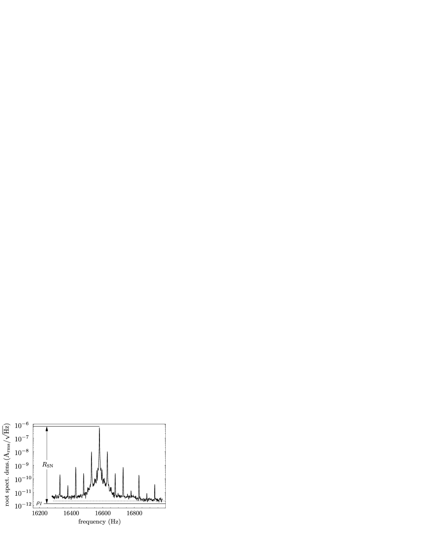
Figure 7: Root power spectrum of the photocurrent when the driving field is in resonance with the Larmor frequency. The data sample was recorded at 54^∘ C under conditions optimized for maximum magnetometric sensitivity with a resolution bandwidth of 1 $\mathrm{Hz}$ (sampling time 1 s). The amplitude measured by the lock-in amplifier corresponds to the upper horizontal line. The amplitude of the central peak is depressed, since it is slightly broadened by the Hanning window used by the FFT spectrum analyzer (see text). The level $\rho_{I}$ is the shot-noise level calculated from the DC-photocurrent. The dashed line marks the rms noise measured at 23 k$\mathrm{Hz}$. The $R_{\mathrm{SN}}$ with respect to the calculated shot-noise level is $5\times 10^{5}$. The rms noise is a factor of 1.55 higher than $\rho_{I}$ resulting in a $R_{\mathrm{SN}}$ of $3.2\times 10^{5}$.

In order to record magnetic resonance lineshapes the lock-in amplifier was synchronized to a reference frequency supplied by a scanning function generator. The data measured by the lock-in (amplitudes of the in-phase and quadrature signals) were transmitted in digital form to a PC, thus avoiding additional noise.

IV Optimization

Although the theory of optical magnetometry is well known bloom , predictions about the real performance of a magnetometer, especially when it is operating in weakly shielded environments, are difficult to make. The performance depends on laser power, rf power, cell size, laser beam profile, buffer-gas pressure, and the temperature-dependent density of Cs atoms. The size of the cells and the buffer gas pressure were dictated by the available cells: We used 20 mm long cells with 20 mm diameter including 45 mbar Ne and 8 mbar Ar with a saturated Cs vapor. Since the cell is oriented at 45^∘ with respect to $\mathbf{B}_{0}$, the transverse spatial resolution was 28 mm. The cross section of the laser beam was limited by the 8 mm apertures of the optical components (polarizers and quarter-wave plates).

IV.1 Intrinsic resolution

Our magnetometer produces a signal which was proportional to the magnetic field changes. The noise of the signal in a perfectly stable field therefore determines the smallest measurable magnetic field change, called the noise equivalent magnetic field (NEM). The NEM is given by the square root, $\rho_{B}$, of the power spectral density, $\rho_{B}^{2}$, of the magnetometer signal, expressed in $\mathrm{T}/\mathrm{Hz}^{1/2}$. The rms noise, $\sigma_{B}$, of the magnetometer in a given bandwidth $f_{\mathrm{bw}}$ is then

$$\sigma_{B}=\rho_{B}\sqrt{f_{\mathrm{bw}}}.$$ (32)

A straightforward way to measure the intrinsic sensitivity would be to extract the noise level from a sampled magnetometer time series via a Fourier transformation. However, that process requires very good magnetic shielding since the measured noise is the sum of the magnetic field noise and the intrinsic noise of the magnetometer. Many studies under well-shielded conditions have been carried out in our laboratory, leading to the result that optical magnetometers are in principle sensitive enough to measure the magnetic field of the human heart. However, the shielding cylinders used in these investigations were too small to accommodate a person. The present study investigates which level of performance can be obtained in a weakly shielded environment with a volume large enough to perform biomagnetic measurements on adults. In the walk-in shielding chamber available in our laboratory the magnetic noise level was about one order of magnitude larger than the strongest magnetic field generated by the heart. In order to compensate for this the actual cardiomagnetic measurements were done with two magnetometers in a gradiometric configuration bison1 . However, the optimal working parameters where determined for a single magnetometer channel only.

Since all time series recorded in this environment are dominated by magnetic field noise, the straightforward way of measuring the intrinsic noise could not be applied. As an alternative approach a lower limit for the intrinsic noise can be calculated using information theory. The so-called Cramér–Rao lower bounds rife gives a lower limit on how precisely parameters, such as phase or frequency, can be extracted from a signal in the presence of a certain noise level. For the following discussion we assume that the signal is a pure sine wave affected by white noise with a power spectral density of $\rho^{2}$. We define the signal-to-noise ratio $R_{\mathrm{SN}}$ as the rms amplitude, $A$, of the sinusoidal signal divided by the noise amplitude, $\sigma$, for the measurement bandwidth, $f_{\mathrm{bw}}$:

$$R_{\mathrm{SN}}=\frac{A}{\sigma}=\frac{A}{\rho\sqrt{f_{\mathrm{bw}}}}\>.$$ (33)

For a magnetometer generating a Larmor frequency proportional to the magnetic field, Eq. (1), the ultimate magnetic sensitivity is limited by the frequency measurement process. The Cramér–Rao lower bound for the variance, $V_{\omega}$, of the frequency measurement rife is used (Appendix VII) to calculate $\rho_{B}$

$$\rho_{B}=\frac{\sigma_{B}}{\sqrt{f_{\mathrm{bw}}}}=\frac{4\sqrt{3}\sqrt{f_{\mathrm{bw}}}}{\gamma_{F}R_{\mathrm{SN}}{}}\>.$$ (34)

For cardiac measurements a bandwidth of $f_{\mathrm{bw}}=100\>\mathrm{Hz}$ is required. This together with a typical value for $R_{\mathrm{SN}}$ of $10^{4}$ results in a magnetic field resolution of $315\>\mathrm{fT}/\mathrm{Hz}^{1/2}$. In order to be competitive with SQUID-based cardiomagnetometers that feature an intrinsic noise of 5…20 $\mathrm{fT}/\mathrm{Hz}^{1/2}$ this level of performance is not sufficient. For that reason we have concentrated on a different mode of operation where the phase signal is measured by digital lock-in detection.

In this mode of operation $\omega_{\mathrm{rf}}$ has a fixed value near the Larmor frequency. The information about the magnetic field is obtained from the phase shift of the magnetometer response at that frequency. The Cramér–Rao bound for a phase measurement of a signal with known frequency is used in Appendix VIII to calculate the NEM for that case:

$$\rho_{B}=\frac{\Gamma_{2}}{\gamma_{F}R_{\mathrm{SN}}\sqrt{f_{\mathrm{bw}}}}\>.$$ (35)

Equations (34) and (35) define the bandwidth:

$$f_{0}=\frac{\Gamma_{2}}{4\sqrt{3}}\>,$$ (36)

for which both approaches yield the same magnetometric sensitivity. For bandwidths larger than $f_{0}$, a phase measurement is more advantageous whereas for bandwidths smaller than $f_{0}$ a frequency measurement gives the higher sensitivity.

IV.2 Bandwidth

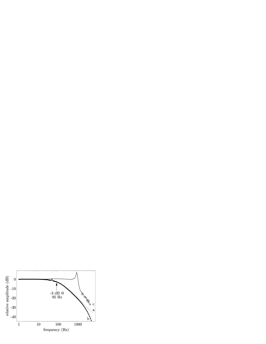
Figure 8: Frequency response of the magnetometer, measured by recording the response to an oscillating magnetic field generated by a test coil. The dots show measured points recorded in free running mode under conditions optimized for maximal magnetometric resolution. (a) Calculated first-order low-pass filter corresponding to a spin polarization lifetime of 1.67 ms. (b) Fitted frequency response taking into account (a) and the $4^{\mathrm{th}}$ order low-pass filter of the lock-in amplifier (time constant $=30~{}\mu\mathrm{s}$). (c) Measured frequency response in the phase-stabilized mode.

In addition to the sensitivity, the bandwidth, i.e., the speed with which the magnetometer signal follows magnetic field changes, is an important feature of a magnetometer. The steady-state solutions of the Bloch equations, $P_{\mathrm{qu}}$ and $P_{\mathrm{ip}}$ [Eqs. (19) and (20)], follow small field changes at a characteristic rate $\Gamma_{2}$, corresponding to a delay time $tau_{S}=\Gamma_{2}^{-1}$. Since the steady state is only reached exponentially, the frequency response is that of a first order low-pass filter [see Fig. 8(a)] with a (-3 dB) cut-off frequency $f_{C}$ given by

$$f_{C}=\frac{1}{2\pi\tau_{S}}=\frac{\Gamma_{2}}{2\pi}=\Delta\nu_{2}\>,$$ (37)

and hence a bandwidth of

$$f_{\mathrm{bw}}=\frac{1}{4\tau_{S}}=\frac{\Gamma_{2}}{4}=\frac{\pi}{2}\,\Delta\nu_{2}\>,$$ (38)

where $\Delta\nu_{2}$ is the half width of the phase signal measured in $\mathrm{Hz}$.

To achieve maximum sensitivity, atomic magnetometers aim at a maximum $\tau_{S}$, at the cost of a reduced bandwidth of typically a few tenths of $\mathrm{Hz}$. A large bandwidth can be obtained by increasing the light power since that leads to shorter $\tau_{S}$ and therefore to higher bandwidth. Larger light powers also increase the S/N ratio but the effect can be overcompensated by magnetic resonance broadening, resulting in a degradation of the magnetometric resolution.

Using feedback to stabilize the magnetic resonance conditions is another way to increase the bandwidth. Figure 8(c) shows the frequency response of the OPM in both the free-running (without feedback) mode and in the phase-stabilized mode where the phase signal is used to stabilize $\omega_{\mathrm{rf}}$ to the Larmor frequency $\omega_{L}$. For large loop gain the bandwidth is mainly limited by loop delays.

A third method to achieve large bandwidths is the so-called self-oscillating mode. In this mode the oscillating signal measured by the photodiode is not demodulated but rather phase-shifted and fed back to the rf-coils. For a 90^∘ phase shift the system then oscillates at the Larmor frequency. In order to measure the magnetic field, the frequency of this oscillation has to be measured. Magnetic field changes then show up — at least theoretically bloom — as instantaneous frequency changes. In practice, reaction times smaller than a single Larmor period have been observed Dyal .

Of the three modes outlined above, the latter two both rely on frequency measurements. The self-oscillating magnetometer provides a frequency that has to be measured. The phase-stabilized magnetometer measures the frequency via a reference frequency locked to the Larmor frequency. As a consequence, both methods suffer from the reduced magnetometric resolution predicted by Eq. (34). Therefore, we have concentrated on the free-running mode of operation for which the magnetometric resolution is given by Eq. (35) and the bandwidth by Eq. (38).

Thanks to the rather high light power required for optimal magnetometric resolution at higher cell temperatures, the cut-off frequency of the magnetometer was 95 $\mathrm{Hz}$. The bandwidth of the device under these conditions can be extracted from the transfer function (Fig. 8(b)) and is about 140 $\mathrm{Hz}$. Because of the time constant of the lock-in amplifier, the measured bandwidth is 10 $\mathrm{Hz}$smaller than the $\pi/2\times 95\>\mathrm{Hz}$ one would expect for a first order low-pass filter [Eq. (38)].

IV.3 Experimental lineshapes

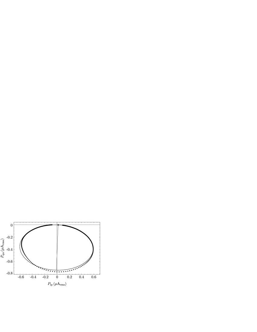
Figure 9: The dots represent a Nyquist plot of the magnetic resonance measured under optimized conditions. The solid line is a fit of Eq. (31) with added offset and phase rotation to the measured data. The fit model assumes a constant magnetic field distribution. The offset is indicated by the dot close to the origin. The short diameter of the ellipse is drawn in order to illustrate the phase rotation of 2.4^∘.

Figure 9 shows a Nyquist plot with experimental data and a model simultaneously fit to the in-phase and quadrature components of the data. The data show a certain asymmetry that can not be reproduced by the model. The Nyquist plots for different magnetic field distributions (Fig. 5) suggest that the asymmetry is caused by inhomogeneous magnetic fields. Unfortunately the models discussed in Sec. II.2 do not fit the data correctly, implying that higher-order gradients cause the deformation of the measured lineshape. The fact that the asymmetry is more pronounced for high rf amplitudes indicates that inhomogeneous rf-fields — causing the different parts of the ensemble to contribute with different widths — have to be considered. Unfortunately, models for such inhomogeneities do not lead to analytic line shapes. An empirical model which assumes the measured resonance consists of a sum of several resonances, each at a different position and with a different width, can be fit to the data. The data can be fit perfectly if the number of subresonances is high enough. However, such fits have a slow convergence and do not provide the needed information about the width and amplitude of the resonance in single fit parameters. For practical reasons (during the optimization more than 2000 spectra were fit) we decided to use the constant magnetic field distribution model for fitting data similar to the ones in Fig. 9.

Magnetic field inhomogeneities have much less influence on the shape of the phase signal resulting in more reliable values for $\Gamma_{2}$. The phase signal represents the speed with which the resonance evolves through the Nyquist plot. Using both the phase signal and the Nyquist plot, the in-phase and quadrature components of the resonance were reconstructed, however, the frequency scaling were given by the phase signal only.

IV.4 Optimization measurements

For the optimization of the NEM given by Eq. (35) the S/N ratio of the lock-in input signal and the linewidth $\Gamma_{2}$ have to be measured. Figure 7 shows a frequency spectrum recorded at the input of the lock-in amplifier using a FFT spectrum analyzer. The frequency $\omega_{\mathrm{rf}}$ was tuned to the center of the magnetic resonance so that the modulation of the photocurrent was at its maximum amplitude. The power spectrum shows a narrow peak at $\omega_{\mathrm{rf}}$ surrounded by noise peaks that characterize the magnetic field noise. Monochromatic magnetic field fluctuations, e.g., line frequency interference, modulate the phase of the measured sine wave and show up in the power spectrum as sidebands. The low frequency flicker noise of the magnetic field thus generates a continuum of sidebands that sum up to the background structure surrounding the peak in Fig. 7. The estimation of the intrinsic sensitivity is based on the assumption that those sidebands would disappear in a perfectly constant magnetic field. The amplitude noise of the signal is mainly due to the electron shot noise in the photodiode, which generates a white noise spectrum. For frequencies which are more than 1 k$\mathrm{Hz}$ away from the resonance, the noise level drops to the white noise floor. The electron shot noise is the fundamental noise level that can not be avoided. The noise spectral density $\rho_{I}$ can be calculated from the DC current $I_{\mathrm{DC}}$ flowing through the photodiode:

$$\rho_{I}=\sqrt{2eI_{\mathrm{DC}}}\>.$$ (39)

At room-temperature the measured rms noise in the spectrum was 5% to 20% above the shot-noise level, depending on induced noise on the photocurrent and the laser frequency stabilization that could cause excess noise in the light intensity. The rms noise rose rapidly for higher temperatures because of the increasing leakage current in the photodiode. Unfortunately, in the experimental setup the photodiodes were in good thermal contact with the Cs cell and, given that the optimal operating temperature of the Cs cells turned out to be in the range of 50^∘ C to 60^∘ C, the photodiode produced an excess noise larger than the shot noise of the photocurrent. Figure 7 shows a spectrum recorded under conditions optimized for maximal magnetometric resolution. At 53^∘ C the measured rms noise was higher than the shot noise by a factor of 1.55. However, this limitation can be overcome easily since the photodiodes do not need to be close to the Cs cell and thus can be operated at room-temperature. In order to avoid the problem of drifting values of $\rho$ during the optimization of $\rho_{B}$, the theoretical shot noise level $\rho_{I}$ was used for $\rho$ in Eq. 33 instead of the measured noise.

The amplitude $A$ of the signal can be extracted from the FFT-spectrum by integrating the spectrum over three points ($\pm 1\>\mathrm{Hz}$) around the center frequency. The procedure was needed since the Hanning window used by the spectrum analyzer to reconstruct the spectrum causes a slight broadening of the central peak. The values calculated in that way are in good agreement with those measured by the lock-in amplifier.

The third parameter needed to calculate the intrinsic sensitivity is the half-width $\Gamma_{2}$ of the magnetic resonance. The value was extracted from a magnetic resonance spectrum recorded by the lock-in amplifier during a frequency sweep of the applied oscillating magnetic field. As discussed in Section IV.3 a constant-gradient model was fit to the data in order to extract $\Gamma_{2}$.

For optimizing in a three-dimensional parameter space, the time for one measurement had to be kept as short as possible. When the lock-in amplifier signal was used as a measure for $A$ [see Eq. (33)] and the noise was calculated from the DC current it was not necessary to record a FFT spectrum for each set of parameters of the optimization procedure. In that way the time for a single NEM measurement was reduced to the 20 s sweep time of $\omega_{\mathrm{rf}}$ plus the time needed to measure the DC current and the temperature of the cell. The measurement was controlled by a PC running dedicated software for recording and fitting the magnetic resonance signals. The amplitude of the rf field, $B_{\mathrm{rf}}$, was changed automatically by the software, resulting in series of typically ten NEMs as a function of $B_{\mathrm{rf}}$. A typical optimization run was made by recording many such series while the system slowly heated up. Repeating those runs for different light powers finally resulted in data for the whole parameter space.

V Results

V.1 Dependence on rf amplitude

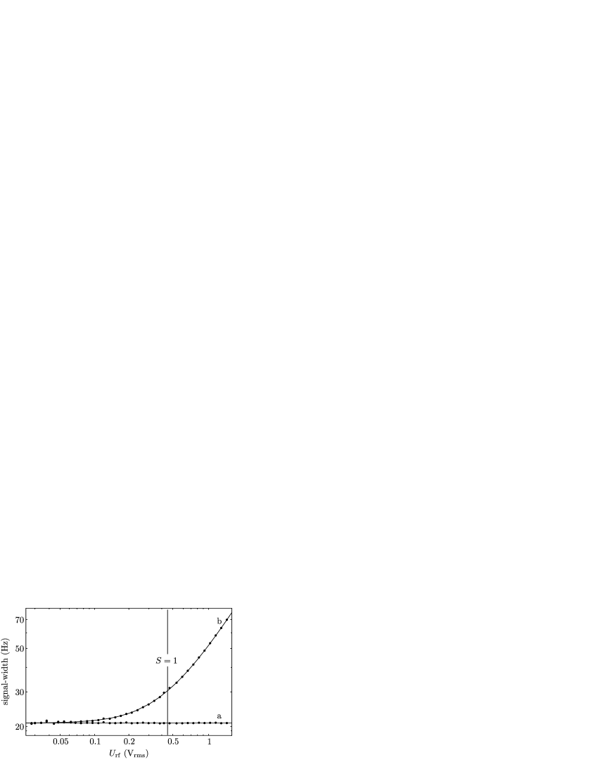
Figure 10: Dependence of the magnetic resonance linewidth on the rf amplitude $U_{\mathrm{rf}}$. The points are extracted from measured magnetic resonance spectra by least squares fitting of model Eq. (31). The phase signal (a) has a constant linewidth whereas the common widths of the in-phase and quadrature signals (b) increase rapidly with rf amplitude. The solid line represents a model fitted to the data that assumed an additional broadening caused by inhomogeneous magnetic fields.

The first study made with the magnetometer examined the dependence of the magnetic resonance on the rf amplitude $B_{\mathrm{rf}}$ measured a series of spectra recorded at room temperature. Figure 10 shows the dependence of the magnetic resonance signal width on the rf amplitude measured by the coil voltage $U_{\mathrm{rf}}$. The width of the phase signal (see Fig. 10) was fit with a constant, whereas the common width of the in-phase and quadrature components were given by Eq. (21). To fit the widths correctly, a constant width had to be added to Eq. (21). The additional constant width can be interpreted as a residual broadening caused by magnetic field inhomogeneities of higher order than the one considered in the line fitting model. The Nyquist plot (see Fig. 9) shows that higher order gradients are present and the excellent agreement in Fig. 10 suggests that they can be treated as an additional broadening.

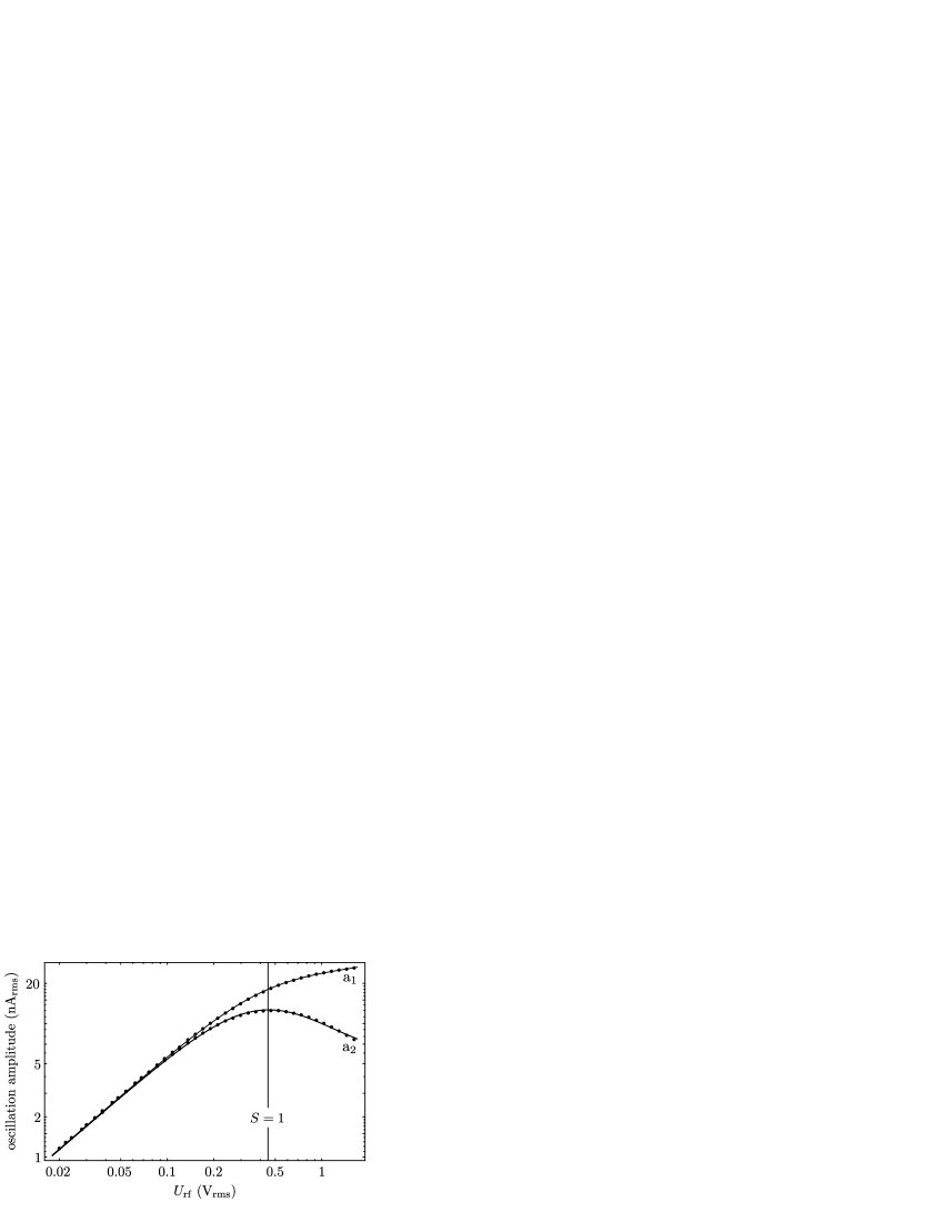
Figure 11: Amplitude of the in-phase ($a_{1}$) and quadrature ($a_{2}$) signals as a function of rf amplitude $U_{\mathrm{rf}}$. The points represent values extracted from measured magnetic resonance spectra. The solid lines show a model fit to the data points (see text). The quadrature amplitude $a2$ is equal to the amplitude of the incoming sine wave on resonance ($\delta=0$).

Figure 11 shows the amplitudes of the in-phase and quadrature magnetic resonance signals. The amplitudes where extracted from the same spectra used for Fig. 10. The fit model used to explain the amplitudes (solid lines in Fig. 11) was based on Eqs. (26) and (27) with a background proportional to $B_{\mathrm{rf}}$. The origin of the background was an inductive pick up of the $\mathbf{B}_{1}$ field by the photocurrent loop which caused an additional phase-shifted sine wave to be superposed on the photocurrent. As discussed in the theory part (see Fig. 4) that lead to an offset in the measured amplitudes of the magnetic resonance signal.

The NEM as a function of rf amplitude is inversely proportional to the quadrature amplitude ($a_{2}$ in Fig. 11), since the linewidth of the phase signal and the shot noise do not change with rf amplitude. The optimal rf amplitude was determined from the data shown in Fig. 11 and corresponds to $S=1$.

V.2 Dependence on temperature and light power

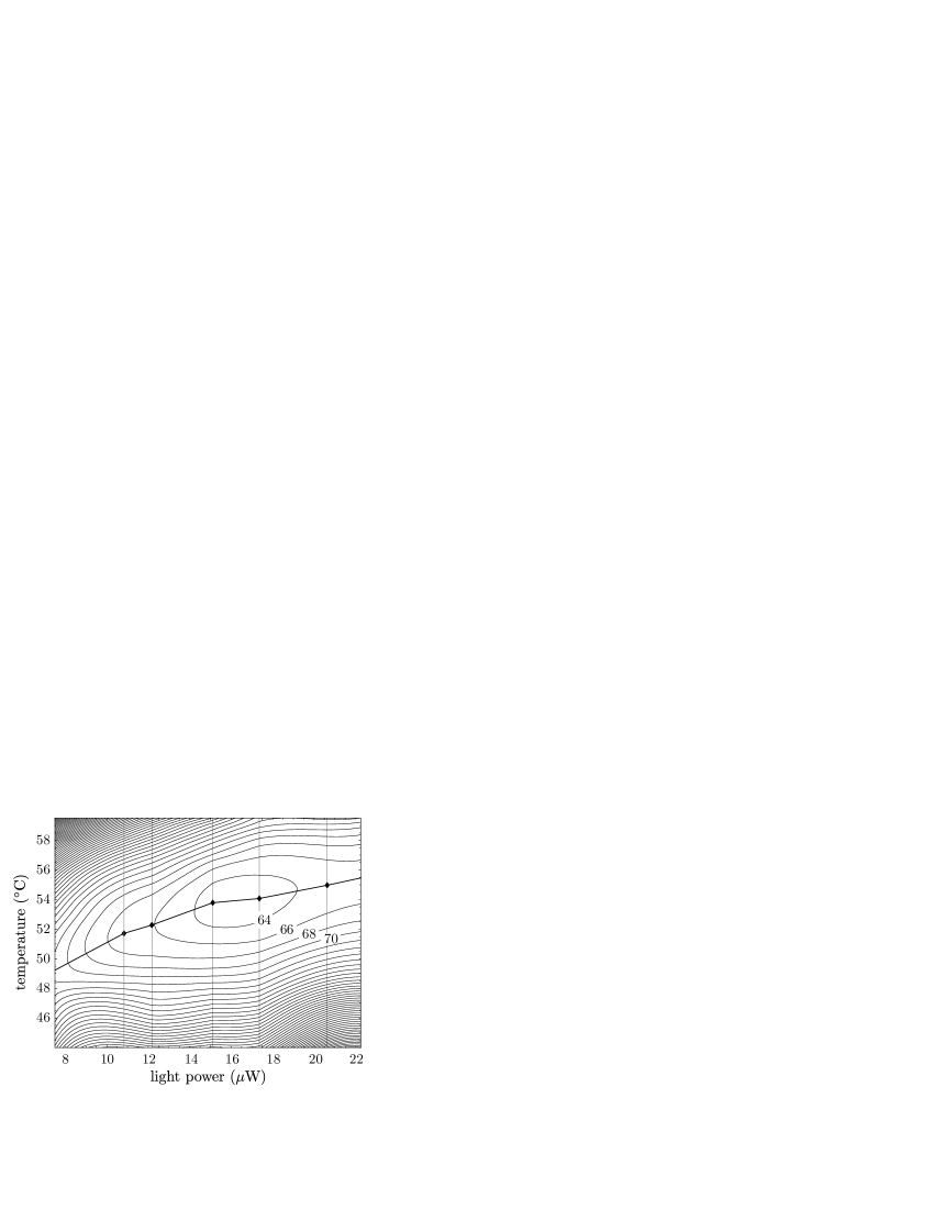
Figure 12: Contour plot of the magnetometric resolution (NEM) as a function of temperature and light power. The map is calculated by numeric interpolation from seven optimization runs (indicated by vertical lines). The labels at the contours mark the NEM in $\mathrm{fT}/\mathrm{Hz}^{1/2}$. The points of minimal NEM for each optimization run are indicated by points. The connecting line is a cut along which the data of Fig. 13 are obtained. Including the variation of the rf amplitude 970 parameter sets were recorded and analyzed to produce the map.

As described in section IV.4 the dependence of the NEM on the temperature was recorded while the system was slowly heated. The rf amplitude was automatically scanned so that for every temperature the optimal rf amplidude could be determined. Figure 12 shows a contour plot of the NEM as a function of temperature and light power. If the light power is increased, the temperature (and hence Cs atom density) has also to be increased to maintain optimal resonance conditions. Figure 13(b) shows the power transmitted through the cell relative to the incident light power. A relative transmission of 0.37 corresponds to an absorption length which matches the cell length. Taking into account losses at the windows, a density corresponding to 1.4 absorption lengths was found to be optimal.

Figure 13: Magnetic resonance parameters as a function of incident light power: (a) shows the width of the phase signal that determines the cut-off frequency of the magnetometer bandwidth; (b) shows the DC transmission through the Cs cell relative to the incident light power; (c) is the signal/noise ratio of the lock-in input signal with respect to calculated shot noise; (d) shows the NEM at the points indicated in Fig. 12.

For each light power the optimal temperature is indicated by a dot in Fig. 12. Plotting the NEM along the optimum temperature power curve, i.e., the curve connecting the dots, results in the plot shown in Fig. 13(d). For light powers below 15 $\mu$W and the corresponding temperatures the sensitivity rapidly degrades. The loss in sensitivity is less pronounced if the power and temperature are chosen above the optimum. Values for $R_{\mathrm{SN}}$ of up to 500 000 (114 dB) were measured at a resolution bandwidth of 1 $\mathrm{Hz}$.

The optimal magnetic field resolution of our magnetometer is reached at a light power of 15 $\mu$W and a temperature of 53^∘ C. With that set of parameters, the usable bandwidth of the magnetometer was determined by a cut-off frequency of about 80 $\mathrm{Hz}$ (see Fig. 13(a)). In order to meet the required 100 $\mathrm{Hz}$ bandwidth a slightly larger light power can be used. All characterizing measurements (cf. Figs. 2, 8, 9, and 7) were therefore performed with a light power of 20 $\mu$W at 54^∘ C.

VI Conclusion

Optimizing the performance of the magnetometer has led to a set of parameters for which the device offers a large sensitivity and a large bandwidth. Both requirements can be met at the same time because of rather large linewidths that turned out to be optimal. Under these conditions the high magnetometric sensitivity relies on the achieved very high signal/noise ratios. The system has the potential to operate at a $R_{\mathrm{SN}}$ of 500000 (Fig. 7) and we hope to be able to demonstrate this once the photodiodes can be removed from the heated Cs cell. However, even using the measured $R_{\mathrm{SN}}$ of 320000, the intrinsic sensitivity of $100\>\mathrm{fT}/\mathrm{Hz}^{1/2}$ is good enough for less demanding cardiomagnetic measurements.

The magnetometer bandwidth of 140 $\mathrm{Hz}$ in the free-running phase-detecting mode (Fig. 8) is high enough for cardiac measurements. The phase-detecting mode avoids the fundamental limitations associated with frequency measurements using short integration times.

An important open experimental question is whether the predicted intrinsic sensitivity can be reached using several of the present OPMs in a higher order gradiometer geometry. With gradiometric SQUID sensors it is possible to achieve NEM value on the order of $20\>\mathrm{fT}/\mathrm{Hz}^{1/2}$ in unshielded environments fenici1 . In future we plan to use cells with spin-preserving wall coatings rather than buffer-gas cells as sensing elements. Coated cells have the advantage that the atoms traverse the volume many times during the spin coherence lifetime, therefore averaging out field inhomogeneities. We are therefore confident that the present limit from field gradients can be overcome and that optical magnetometers can reach an operation mode limited by their intrinsic sensitivity.

VII Appendix A: The Cramér–Rao bound for frequency measuring magnetometers

For the measurement of the frequency $\omega$ of a sine wave with a rms amplitude $A$ sampled at $N\gg 1$ points separated by time intervals $T_{s}$ the Cramér–Rao lower bound for the variance $V_{\omega}$ of $\omega$ in the presence of white Gaussian amplitude noise of variance $\sigma^{2}$ is given by rife :

$$V_{\omega}=\frac{12\sigma^{2}}{A^{2}T_{M}^{2}N},$$ (40)

where $T_{M}=NT_{s}$ is the total time interval for one frequency determination. The bandwidth on the input side of the lock-in amplifier is therefore $F_{\mathrm{bw}}=1/2T_{s}=N/2T_{M}$, that at the output is $f_{\mathrm{bw}}=1/2T_{M}$. With the definition of the signal-to-noise ratio, Eq. (33), $V_{\omega}$ can be expressed independently of the number of samples:

$$V_{\omega}=\frac{12\rho_{i}^{2}F_{\mathrm{bw}}}{A^{2}T_{M}^{2}N}=\frac{6}{R_{\mathrm{SN}}^{2}T_{M}^{3}}.$$ (41)

Ideal measuring processes are limited by that condition only. Frequency measurements by a FFT with peak interpolation is a Cramér–Rao bound limited measuring process rife .

From that bound a lower limit for the performance of a frequency measuring magnetometer can be derived. The so-called self-oscillating $M_{x}$ magnetometer bloom is of this type since it supplies an oscillating signal with a frequency proportional to the magnetic field. With Eq. (1) it follows that the root spectral density of the measurement noise $\rho_{B}$ is given by:

$$\rho_{B}=\sqrt{\frac{V_{B}}{f_{\mathrm{bw}}}}=\frac{4\sqrt{3}\sqrt{f_{\mathrm{bw}}}}{\gamma_{F}R_{\mathrm{SN}}{}}.$$ (42)

VIII Appendix B: The Cramér–Rao bound for phase measuring magnetometers

The Cramér–Rao lower bound for the measurement of the phase of a signal with known frequency is given by rife :

$$V_{\varphi}=\frac{\sigma^{2}}{A^{2}N}\>.$$ (43)

An example of a measurement process limited only by that condition is the lock-in phase detection where the phase is calculated from the in-phase and quadrature outputs of the lock-in amplifier [see Eq. (23)]. In order to calculate the variance $V_{\varphi}$ of the phase measurement we assume a white amplitude noise spectrum with a power spectral density $\rho^{2}$:

$$V_{\varphi}=\frac{\rho^{2}}{A^{2}2T_{M}}\>.$$ (44)

Using this expression and the definition of $R_{\mathrm{SN}}$ [Eq. (33)], Eq. (44) can be written as

$$\sigma_{\varphi}^{2}=V_{\varphi}=\frac{\rho^{2}f_{\mathrm{bw}}}{A^{2}}=\frac{f_{\mathrm{bw}}}{R_{\mathrm{SN}}^{2}}\>.$$ (45)

From the measured phase $\varphi$, the detuning $\delta=\omega_{\mathrm{rf}}-\omega_{L}$ can be derived. For $\varphi\ll 1$, Eq. (23) leads to $\delta\approx\Gamma_{2}\varphi$. Using Eq. (1), the detuning can be expressed as a magnetic field difference $\Delta B=\delta/\gamma$ which leads, together with Eq. (45), to the magnetic field resolution $\sigma_{B}$:

$$\sigma_{B}=\frac{\sigma_{\delta}}{\gamma_{F}}=\frac{\sigma_{\varphi}\Gamma}{\gamma_{F}}=\frac{\Gamma\sqrt{f_{\mathrm{bw}}}}{\gamma_{F}R_{\mathrm{SN}}\sqrt{f_{\mathrm{bw}}}}\>.$$ (46)

The root spectral density of the noise in the $\Delta_{B}$ measurement, $\rho_{B}=\sigma_{B}/f_{\mathrm{bw}}^{1/2}$, is thus given by:

$$\rho_{B}=\frac{\Gamma}{\gamma_{F}R_{\mathrm{SN}}\sqrt{f_{\mathrm{bw}}}}\>.$$ (47)

References

- (1) W. Andrä and H. Nowak eds., Magnetism in Medicine (Wiley-VCH, Berlin 1998).
- (2) J. P. Wikswo, “Biomagnetic sources and their models,” in Proceedings of the Seventh International Conference on Biomagnetism, New York, 13–18 August 1989, S. J. Williamson, ed., p. 1 (1989).
- (3) D. Cohen, E. A. Edelsack, and J. E. Zimmerman, “Magnetocardiograms taken inside a shielded room with a superconducting point-contact magnetometer,” Appl. Phys. Lett. 16, 278 (1970).
- (4) A. L. Bloom, “Principles of Operation of the Rubidium Vapor Magnetometer,” Appl. Opt. 1, 61 (1962).
- (5) J. Dupont-Roc, S. Haroche, and C. Cohen-Tannoudji, “Detection of very weak magnetic fields (10–9 Gauss) by 87Rb-zero-field level crossing resonances,” Phys. Lett. 28A, 638 (1969).
- (6) E. B. Alexandrov and V. A. Bonch-Bruevich, “Optically pumped atomic magnetometers after 3 decades,” Opt. Eng. 31(4), 711–717 (1992).
- (7) A. Kastler, “The Hanle Effect and its use for the measurement of very small magnetic fields,” Nucl. Instr. Meth. 110, 259–265 (1973).
- (8) D. Budker, D. F. Kimball, S. M. Rochester, V. V. Yashchuk, and M. Zolotorev, “Sensitive magnetometry based on nonlinear magneto-optical rotation,” Phys. Rev. A 63, 043 403 (2000).
- (9) M. N. Livanov, A. N. Kozlov, S. E. Sinelnikova, J. A. Kholodov, V. P. Markin, A. M. Gorbach, and A. V. Korinewsky, “Record of the Human Magnetocardiogram by the Quantum Gradiometer with Optical Pumping,” Adv. Cardiol. 28, 78 (1981).
- (10) S. Kanorsky, S. Lang, S. Lücke, S. Ross, T. Hänsch, and A. Weis, “Millihertz magnetic resonance spectroscopy of Cs atoms in body-centered-cubic 4He,” Phys. Rev. A 54, R1010 (1996).
- (11) G. Bison, R. Wynands, and A. Weis, “A laser-pumped magnetometer for the mapping of human cardiomagnetic fields,” Appl. Phys. B 76 (2003).
- (12) G. Bison, R. Wynands, and A. Weis, “Dynamical mapping of the human cardiomagnetic field with a room-temperature, laser-optical sensor,” Optics Express 11 (2003).
- (13) K. L. Corwin, Z.-T. Lu, C. F. Hand, R. J. Epstain, and C. E. Wieman, “Frequency-stabilized diode laser with the Zeeman shift in an atomic vapor,” Appl. Optics 37(15) (1998).
- (14) D. C. Rife and R. R. Boorstyn, “Single-Tone Paramter Estimation from Discrete-Time Observations,” IEEE Transactions on Information Theory 20(5) (1974).
- (15) P. Dyal, R. T. J. Jr., and J. C. Giles, “Response of self-oscillating rubidium vapor magnetometers to rapid field changes,” Rev. Sci. Instrum. 40(4) (1969).
- (16) I. Tavarozzi, S. Comani, C. D. Gratta, G. L. Romani, S. D. Luzio, D. Brisinda, S. Gallina, M. Zimarino, R. Fenici, and R. D. Caterina, “Magnetocardiography: current status and perspectives. Part I: Physical principals and instrumentation,” Ital. Heart J. 3, 75 (2002).