Nanoporous compound materials for optical applications –
Microlasers and microresonators

1 Introduction

Since many decades nanoporous materials, for example zeolites, play an eminently important role in the catalysis of oil refining and petrochemistry. On the other hand, molecular sieve materials began also to attract some attention as optical material in last years. It was realized that their nanometer size pores allow to host guest molecules giving so substance to a new class of optical material with properties which neither the host, nor the guest alone could ever possess. In this way new pigments and luminophores were realized as well as novel optically nonlinear and switching materials. The various actually realized materials are reviewed in this book in chapter Nanoporous compound materials for optical applications – Material design and properties.

A closer look at the approach of arranging molecules in an ordered framework of pores reveals a series of aspects of fundamental interest: For example, the stereometric restrictions which the pore framework imposes on the motional degrees of freedom of the enclosed molecules reduces their diffusion to one dimensional diffusion in channel pores [1]. Or, as with the concentration also the average distance between two guest molecules is controlled, their dipolar near field interaction can so be adjusted. In optimal circumstances optical excitation energy can then be transferred nonradiatively over distances of several micrometers [2]. That are just two examples of new phenomena in molecular sieves, which at this moment are still studied to achieve full understanding, and which will soon find their way into applications in science and technology.

In this chapter we will be concerned with another new optical application of nanoporous compound materials, namely microlasers in which light is generated by organic dyes embedded in wavelength size resonators of molecular sieve material. In these laser devices the dye molecules are enclosed in nanometer size channel pores of the molecular sieve, whereas the crystalline sieve material itself which forms the resonator has exterior dimensions on the order of a few micrometers. Figure 1 illustrates the arrangement of the molecular dye dipoles which are aligned in the pores of a hexagonally shaped AlPO₄-5 molecular sieve host.

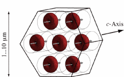
Figure 1: Schematic picture of the arrangement of the molecular dye dipoles in the channel pores of the hexagonal molecular sieve host crystal AlPO₄-5. The spatial cosine-square emission efficiency of a dipole is represented as doughnut shaped surface around the dipole axes.

In this example of molecular sieve material the channel pores point to the direction of the crystal $c$-axis. If the enclosed species of dye molecules have an elongated shape and exhibit a transition dipole moment along their elongation axis, then the dipoles end up oriented parallel to the host $c$-axis as well.

A dipole can not emit in direction of its axis. Therefore the emission of the dipoles shown in Fig. 1 occurs in a plane normal to the host crystal $c$-axis. Once the light emitted by the dipoles arrives at the boundary of the molecular sieve crystal, part of it is reflected back into the material. In fact, given the hexagonal geometry there is even a bundle of directions for which total internal reflection occurs. Figure 2 illustrates how optical rays of this bundle loop around the crystal, and, reflected by the hexagonal sides, form a whispering gallery mode.

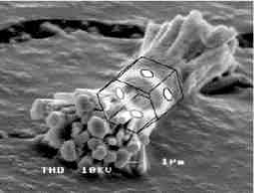
Figure 2: Light which is confined by total internal reflection at the hexagonal boundaries can circulate inside the molecular sieve crystal as whispering gallery mode.

In that way regularly shaped crystals of molecular sieve hosts form microresonator environments for the light emission of inclosed dye molecule guests, and if the molecules provide sufficient optical gain, laser oscillations will build up [3].

Light emission in a microcavity environment, however, is in many respect different from the familiar emission into free space, such as fluorescence. In fact, this difference can be striking. For example, to achieve laser action in a conventional millimeter size (or larger) laser resonator the pump must overcome a certain threshold. In a microlaser in which the resonator is of the size of a few wavelengths, however, lasing can occur without threshold. That means that every absorbed pump quantum is transformed into a laser photon. Therefore, in order to appreciate the significance of light generation in molecular sieve based microlasers, we need to understand the differences between the emission processes of a molecule in a free space environment as opposed to emission in a microcavity environment.

In the following we will review spontaneous as well as stimulated light emission of molecules, and we will show that the respective emission rate is not an inherent molecular property, but is a function of its environment, or more precisely, of the mode density of the electromagnetic field. This becomes apparent when in the distance of a half to a few wavelengths of the molecule mirrors exist. But this is indeed exactly the situation of here discussed dye molecules which are enclosed in a molecular sieve microresonator.

On the other hand, we know that emission and absorption of radiation is accompanied by a transition of the molecule from a state with energy $E_{1}$ to a state with energy $E_{2}$. The frequency of the emitted or absorbed light is then $\omega=\lvert E_{1}-E_{2}\rvert/\hbar$, where $\hbar$ is Planck’s constant. The presence of $\hbar$ clearly shows that emission and absorption of light is intrinsically a quantum mechanical process. Therefore our discussion will have to involve the quantum aspects of the interaction of the dye molecules with the light field, as well as the quantum nature of the light field itself.

The situation is even more peculiar because the resonators of the molecular sieve microlasers have a hexagonal outline. For a hexagonal resonator one can not find an orthogonal coordinate system in which the wave equation can be solved by the usual method of separation of variables. Thus we will have to discuss the properties of microresonators in view of this impediment.

In consideration of these facts we have organized the discussion in the following way: In the first section we introduce the concept of modes of the electromagnetic field as its countable degrees of freedom, and based on this, we introduce the quantized optical field. In the next section fluorescence, i.e. spontaneous emission in a free space environment is discussed, and the frame is set for the treatment of cavity effects in the next section, in which spontaneous emission in a resonator environment is examined. Then the effect of a resonator on stimulated emission and laser action are surveyed. After this we characterize the peculiarities of microresonators, and finally we present the most recent achievements and realizations of molecular sieve microlasers.

2 The concept of “modes” of the electromagnetic field and its quantization

In optics in general, and particularly when lasers are involved, the notion of modes is ubiquitous. As this term is used in many different and disparate circumstances it is necessary to define the term for further usage. In this section we give a short tutorial introduction of the concept of modes of the electromagnetic field, and we show the important role the mode concept plays in the procedure of the canonical quantization of the field. An account of the mode structure of resonators and particularly microresonators is then presented in section 6.

2.1 The dynamics of the classical field

A convenient way to introduce the mode concept is to consider a simple realization of the electromagnetic field, for example a source-free field. We can think of it as the field that subsists after a source located far away has stopped to emit. After the emission stopped, the classical field evolution is governed by Maxwell’s equation in the following form (cgs-units):

$$\vec{\nabla}\cdot\vec{E}=0 \vec{\nabla}\times\vec{E}=-\frac{1}{c}\frac{\partial\vec{B}}{\partial t}$$

$$\vec{\nabla}\cdot\vec{B}=0 \vec{\nabla}\times\vec{B}=\;\;\frac{1}{c}\frac{\partial\vec{E}}{\partial t}$$ (1)

2.2 Discretizing fields – Random fields

Most practical light sources, such as incandescent lamps or light emitting diodes LEDs (though not lasers), emit a nondeterministic, chaotic field, i.e. a field whose spatio-temporal evolution can only be described in statistical terms. In communication engineering terms such a field is referred to as a noise field. We like to point out that we can understand important features of those fields in classical terms. It is thus not necessary to enter the quantum world in order to encounter nondeterministic fields. In order to keep the mathematics simple, it is convenient to deal with a field occupying a discrete, instead of a continuous number of degrees of freedom.

The trick usually used to achieve discretization consists in confining the field into a finite volume $V$. At the end, the limit $V\rightarrow\infty$ can be carried out, if necessary. Confinement to a finite volume $V$ allows us to represent the spatial component of the field as a series (superposition) of a discrete number of functions. As (1) is a system of linear equations of the fields $\vec{E}$ and $\vec{B}$ we can always represent a solution as a linear superposition of field functions. Of course it is convenient to choose a complete and orthonormal set of functions $\{\varphi_{i}(\vec{r})\}$, that also fulfill eventually given boundary conditions. These functions are called (spatial) modes. Thus a mode of the classical electromagnetic field is characterized by the following properties:

• $\{\varphi_{i}(\vec{r})\}$ orthonormal:
  

  $$\int_{V}\varphi_{m}^{\ast}(\vec{r})\varphi_{n}(\vec{r}){\rm d}V=\delta_{mn}$$ (2)

• $\{\varphi_{i}(\vec{r})\}$ complete:
  

  $$E_{x}(\vec{r},t) = \sum_{i}C_{i}\varphi_{i}(\vec{r}){\rm e}^{-{\rm i}\omega_{i}t}+\sum_{i}C_{i}^{\ast}\varphi_{i}^{\ast}(\vec{r}){\rm e}^{{\rm i}\omega_{i}t}$$ (3)

  $$E_{x}(\vec{r},t) = \quad\;\qquad E_{x}^{(+)}\qquad+\qquad E_{x}^{(-)}$$ (4)

• $\{\varphi_{i}(\vec{r})\}$ satisfies the spatial boundary conditions given by the shape of volume $V$.

Obviously $E_{x}^{(-)}=\bigl{(}E_{x}^{(+)}\bigr{)}^{\ast}$ (with ^∗ we denote complex conjugation). The sets $\{C_{i}\}_{x,y,z}$ are discrete, and they now represent the complete information about the field. In a deterministic field the individual $\{C_{i}\}_{x,y,z}$ are fixed complex numbers. For a nondeterministic field, however, the $\{C_{i}\}_{x,y,z}$ represent random variables. Thus for a stationary field they are defined in terms of probability functions:

$$p\,(\,\{C_{i}\}\,)=p\,(C_{1},C_{2},C_{3},\;\ldots\;)$$ (5)

If we consider a function $F$ that depends on the random field, say $E$, or $E^{(+)}$, then we can only express $F$ in statistical terms, that means we can only assign expectation values:

$$\langle\,F(E^{(+)})\,\rangle=\int_{V}p\,(\,\{C_{k}\}\,)\;F\,[E^{(+)}(\{C_{k}\})]\,\prod_{k}\,{\rm d}^{2}C_{k}$$ (6)

In contrast to a thermodynamic situation in which the expectation values are sharply peaked, an experimental realization of $F$ in optics can significantly differ from the expectation value $\langle\,F\,\rangle$.

2.3 The classical Hamiltonian of the source-free field

For a source-free field the classical Hamiltonian $H$ can be interpreted as the total energy of the field. As we have constrained the field to the Volume $V$, the total energy is given by [4]:

$$H=\frac{1}{2}\,\int_{V}[\varepsilon_{0}\vec{E}^{2}(\vec{r},t)+\frac{1}{\mu_{0}}\vec{B}^{2}(\vec{r},t)]\;{\rm d}V\quad.$$ (7)

In the following we will show that the Hamiltonian (7) can be represented as a sum of terms that are analogous to a harmonic oscillator (The thoughtful reader anticipates the reason…). For that purpose we express the fields $\vec{E}$ and $\vec{B}$ in terms of their potential.

2.3.1 The potential of the free field

We recall that Maxwell’s equations of a source free field are gauge invariant. In the case we discuss here we choose the Coulomb gauge, and as a result we obtain a purely transverse field potential $\vec{A}$:

$$\vec{\nabla}\;\cdot\;\vec{A}\;=\;0\quad.$$ (8)

The electric and magnetic fields are related to the potential according to:

$$\vec{E}(\vec{r},t)=-\frac{\partial}{\partial t}\vec{A}(\vec{r},t)\quad,\quad\vec{B}(\vec{r},t)=\vec{\nabla}\,\times\,\vec{A}(\vec{r},t)\quad.$$ (9)

Inserting this into (1) we obtain the wave equation

$$\vec{\nabla}^{2}\vec{A}\,-\,\frac{1}{c^{2}}\,\frac{\partial^{2}}{\partial t^{2}}\vec{A}\,=\,\vec{0}\quad.$$ (10)

2.3.2 Discretization procedure for the potential A

We follow the thread outlined in section 2.2, and to keep things simple, we consider a cube shaped volume $V$ with an edge length of $L$. With this conditions the discretization of $\vec{A}$ acquires the form of a Fourier series (plane wave expansion):

$$\vec{A}(\vec{r},t)=\frac{1}{\sqrt{\varepsilon_{0}}\;L^{3/2}}\sum_{\vec{k}}\vec{\cal A}_{\vec{k}}(t)\exp({\rm i}\vec{k}\cdot\vec{r})\quad,$$ (11)

where the wave vector $\vec{k}$ has the components

$$k_{1}=2\pi n_{1}/L\quad \quad n_{1}=0,\;\pm 1,\;\pm 2,\;\ldots$$ ,

$$k_{2}=2\pi n_{2}/L\quad \quad n_{2}=0,\;\pm 1,\;\pm 2,\;\ldots$$ , (12)

$$k_{3}=2\pi n_{3}/L\quad \quad n_{3}=0,\;\pm 1,\;\pm 2,\;\ldots\quad,$$ ,

and $\sum_{\vec{k}}$ extends over the modes indexed by $n_{1},n_{2},n_{3}$. The chosen normalizing factor will soon prove to be useful. Evaluation of the gauge relation (8) results in

$$\frac{\rm i}{\sqrt{\varepsilon_{0}}\;L^{3/2}}\sum_{\vec{k}}\vec{k}\,\cdot\,\vec{\cal A}_{\vec{k}}(t)\exp({\rm i}\vec{k}\cdot\vec{r})\;=\;0$$ (13)

for all $\vec{r}$. This is only possible when

$$\vec{k}\;\cdot\;\vec{\cal A}_{\vec{k}}(t)\;=\;0\;,$$ (14)

thus $\vec{k}\bot\vec{\cal A}_{\vec{k}}$ (i.e. transversal field). As the potential $\vec{A}(\vec{r},t)$ assumes real values, the coefficients $\vec{\cal A}_{\vec{k}}$ observe

$$\vec{\cal A}_{-\vec{k}}(t)=\vec{\cal A}_{\vec{k}}^{\ast}(t)\;.$$ (15)

In addition, wave equation (10) must be satisfied, resulting in

$$\left(\frac{\partial^{2}}{\partial t^{2}}+\omega_{\vec{k}}^{2}\right)\;\vec{\cal A}_{\vec{k}}(t)=0\;,$$ (16)

with $\omega_{\vec{k}}=ck$. The general solution of this ordinary differential equation is represented as

$$\vec{\cal A}_{\vec{k}}(t)=\>\vec{c}_{\vec{k}}\;{\rm e}^{-{\rm i}\omega_{\vec{k}}t}\;+\;\vec{c}_{-\vec{k}}^{\>\ast}\;{\rm e}^{{\rm i}\omega_{\vec{k}}t}\;.$$ (17)

As (14) fixes the transversal character of each plane wave mode, only two components (the polarization components) of the vector $\vec{\cal A}_{\vec{k}}(t)$ are at free disposition. In order to simplify the notation let us agree to let index ${}_{\vec{k}}$ point to $n_{1},n_{2},n_{3}$ (see (12)), as well as to the polarization components $\vec{\xi}_{1},\vec{\xi}_{2}$. To remember this, we will from now on refer to the corresponding index as ${}_{\bf k_{\xi}}$. With this notation we can write for the potential

$$\vec{A}(\vec{r},t)=\frac{1}{\sqrt{\varepsilon_{0}}L^{3/2}}\sum_{\bf k_{\xi}}[c_{\bf k_{\xi}}{\rm e}^{{-\rm i}\omega_{\bf k_{\xi}}t}+c_{-\bf k_{\xi}}^{\ast}{\rm e}^{{\rm i}\omega_{\bf k_{\xi}}t}]{\rm e}^{{\rm i}\vec{k}\cdot\vec{r}}\quad,$$ (18)

and with

$$u_{\bf k_{\xi}}(t)=c_{\bf k_{\xi}}\,{\rm e}^{-{\rm i}\omega_{\bf k_{\xi}}t}$$ (19)

we get

$$\vec{A}(\vec{r},t)=\frac{1}{\sqrt{\varepsilon_{0}}L^{3/2}}\sum_{\bf k_{\xi}}[u_{\bf k_{\xi}}(t){\rm e}^{{\rm i}\vec{k}\cdot\vec{r}}+u_{\bf k_{\xi}}^{\ast}(t){\rm e}^{{-\rm i}\vec{k}\cdot\vec{r}}].$$ (20)

By inserting (20) in (9), we can express the electric and magnetic field as a sum of mode functions

$$\vec{E}(\vec{r},t) = \frac{\rm i}{\sqrt{\varepsilon_{0}}L^{3/2}}\sum_{\bf k_{\xi}}\omega_{\bf k_{\xi}}[u_{\bf k_{\xi}}(t){\rm e}^{{\rm i}\vec{k}\cdot\vec{r}}-{\rm c.c.}]$$ (21)

$$\vec{B}(\vec{r},t) = \frac{\rm i}{\sqrt{\varepsilon_{0}}L^{3/2}}\sum_{\bf k_{\xi}}[u_{\bf k_{\xi}}(t)(\vec{k}\times\vec{\xi}){\rm e}^{{\rm i}\vec{k}\cdot\vec{r}}-{\rm c.c.}]$$ (22)

where with $\vec{\xi}$ we represent the polarization unit-vector. We note that the total information on the (classical) field is now contained in the functions $u_{\bf k_{\xi}}(t)$ (19).
Note: To avoid confusion, we have to point to a minor inconsistency in the notation: As is typical for expressions of the magnetic field, the vector product in (22) reshuffles spatial and polarization indices so that the correct expression in fact consists of two sums containing the polarization vector. The resulting expression looks bulky, and requires some consideration. For this tutorial we prefer to emphasize the basic mathematical structure. So we choose this visually intuitive representation although the indices are not correctly rendered. To obtain the correct result one may work out the procedure in the component notation of (20) and (9).

2.3.3 The mode density

Let us return for a moment to the volume $L^{3}$ we considered for deriving the mode expansion (11), which was a cube with edges oriented along the coordinate axes $(x_{1},x_{2},x_{3})$. According to (11) we can expand the field in this cube in a 3-dimensional set of running modes $\{k_{1}\},\{k_{2}\},\{k_{3}\}$ [cf. (12)]. Along the $x_{1}$-axis we have the modes labeled by $k_{1}=2\pi n_{1}/L;\;(n_{1}=\pm 1,\pm 2,\dots)$; because we consider only running modes (travelling waves), we omit $n_{1}=0$. In the interval between $k_{1}$ and $k_{1}+{\rm d}k_{1}$ we find ${\rm d}n_{1}$ modes, where ${\rm d}n_{1}={\rm d}k_{1}\;L/2\pi$. The analogous applies for the other directions.

Figure 3: Mode distribution in $\vec{k}$-space scaled by multiplication with $\frac{L}{2\pi}$. Each dot corresponds to a wavevector $\vec{k}$ which represents two independent, orthogonally polarized waves.

According to Fig. 3 we can specify the number of modes in the interval between $\lvert\vec{k}\rvert$ and $\lvert\vec{k}+\vec{{\rm d}k}\rvert$ simply by counting the dots in the volume of the corresponding spherical shell, which amounts to $4\pi k^{2}\;{\rm d}k\cdot 2$ (factor 2 because there are two independent polarization states associated with each $\vec{k}$). Considering the scaling of the axes in Fig. 3 we can use this to express the number of modes in Volume $V=L^{3}$ as

$$\text{Number of modes in $V$}=2\cdot 4\pi k^{2}{\rm d}k\;\left(\frac{L}{2\pi}\right)^{3}\;.$$ (23)

The mode density $\rho(k){\rm d}k$, that is the number of modes in interval $\lvert\vec{{\rm d}k}\rvert$ per Volume $V=L^{3}$, is then given by

$$\rho(k){\rm d}k=\frac{\text{\# of modes in $V$}}{V}=\frac{k^{2}\;{\rm d}k}{\pi^{2}}\;.$$ (24)

With $k=\frac{\omega}{c}$ we obtain

$$\rho(\omega){\rm d}\omega=\frac{\omega^{2}}{c^{3}\pi^{2}}\;{\rm d}\omega\;.$$ (25)

This is known as the free space mode density. Note that $\rho(\omega)$ represents the volume normalized density of modes, i.e. the units of $\rho(\omega)$ are number of modes / (frequency $\times$ volume).

Let us now consider a linear function $\zeta$ of the field, which thus can be represented as a sum over the field modes $\vec{k}$ as

$$\zeta=\sum_{k_{1},k_{2},k_{3}}\zeta(\vec{k})\;.$$ (26)

For a large cube, $L\to\infty$, the sum over the discrete set of modes has to be transformed into an integral, which has to sum over a measure that is a density

$$\frac{1}{L^{3}}\sum_{k_{1},k_{2},k_{3}}\zeta(\vec{k})\longrightarrow\frac{1}{(2\pi)^{3}}\,\int{\rm d}^{3}k\;\zeta({\vec{k}})\;.$$ (27)

Switching to spherical coordinates ${\rm d}^{3}k=k^{2}{\rm d}k\;\sin\theta\,{\rm d}\theta\;{\rm d}\phi$, where $\phi$ denotes the azimuthal and $\theta$ the polar angle of $\vec{k}$, and transforming this equation to frequency space $\omega$ we obtain observing $k=\omega/c$

$$\frac{1}{L^{3}}\sum_{k_{1},k_{2},k_{3}}\zeta(\vec{k})\longrightarrow\frac{1}{(2\pi)^{3}}\,\int{\rm d}\omega\;\frac{\omega^{2}}{c^{3}}\;\int_{0}^{\pi}{\rm d}\theta\,\sin\theta\,\int_{0}^{2\pi}{\rm d}\phi\;\zeta({\vec{k}})$$ (28)

In this representation we take into account that $\zeta$ can depend on the polarization, which can be expressed as $\zeta=\zeta(\phi,\theta,k)$. Also, $\zeta$ allows us to introduce $\vec{k}$-space structure functions into the mode counting sum, so that the mode density can be calculated for arbitrary boundary conditions. Note that the procedure relies on certain properties of the field, one of which is (7). This equation expresses energy conservation, thus the above calculated mode density refers to undamped modes. The situation with microlasers, where sources of the field are present and the modes are damped, is more intricate and is discussed in section 6.

2.3.4 The classical Hamiltonian of the source free field

Let us insert the electric field (21) and the magnetic field (22) into the energy (7) (note that $\int_{L^{3}}{\rm e}^{{\rm i}(\vec{k}-\vec{k^{\prime}})\cdot\vec{r}}{\rm d}^{3}r=L^{3}\,\delta_{\vec{k}\vec{k^{\prime}}}$), then we obtain the Hamiltonian

$$H=2\sum_{\bf k_{\xi}}\omega^{2}\,|u_{\bf k_{\xi}}(t)|^{2}\;.$$ (29)

The energy appears here as the sum of the energy of each mode. This is intuitive, and at this point we could stop satisfied with the result. However, there is one thing that experience revealed: As elegant it might be, expression (29) does not lend itself to an idea that opens a viable way for the quantization of the electromagnetic field.

Although at this time it looks utterly artificial, but the following substitution proved to be a wonderfully prolific device:

$$q_{\bf k_{\xi}}(t) = \qquad\;\;[u_{\bf k_{\xi}}(t)+u_{\bf k_{\xi}}^{\ast}(t)]$$ (30)

$$p_{\bf k_{\xi}}(t) = -{\rm i}\omega_{\bf k_{\xi}}[u_{\bf k_{\xi}}(t)-u_{\bf k_{\xi}}^{\ast}(t)]$$ (31)

At this time this expressions can be regarded as the definition for the functions $q$ and $p$ that, as can be shown, satisfy the relations $\dot{q}_{\bf k_{\xi}}=p_{\bf k_{\xi}}$ and $\dot{p}_{\bf k_{\xi}}=-\omega^{2}q_{\bf k_{\xi}}$. Thus the functions $q$ and $p$ evolve in analogy to the canonical position and momentum variables of the harmonic oscillator: In fact, inserting (30) and (31) in (29), we obtain the expression

$$H=\frac{1}{2}\sum_{\bf k_{\xi}}[p_{\bf k_{\xi}}^{2}(t)+\omega_{\bf k_{\xi}}^{2}q_{\bf k_{\xi}}^{2}(t)]\quad,$$ (32)

which has the same form as the Hamiltonian of a series of independent (not coupled) harmonic oscillators.
What do we have achieved so far?

1. By restricting the fields to a finite Volume $V$, the potential of the electromagnetic field was decomposed in a discrete, although infinite, series of spatial modes.

2. Each spatial mode was associated with a harmonic oscillator.

3. That this is a sound result can be seen by verifying the canonical equations of motion, which indeed show that $\partial H/\partial p_{\bf k_{\xi}}=\dot{q}_{\bf k_{\xi}}$ and $\partial H/\partial q_{\bf k_{\xi}}=-\dot{p}_{\bf k_{\xi}}$.

To be complete we write the fields expressed in terms of $q$ and $p$ :

$$\vec{A}(\vec{r},t) = {\textstyle\frac{1}{2\sqrt{\epsilon_{0}}L^{\frac{3}{2}}}}\sum_{\bf k_{\xi}}\left\{\!\left[q_{\bf k_{\xi}}(t)+\!\!{\textstyle\frac{\rm i}{\omega_{\bf k_{\xi}}}}p_{\bf k_{\xi}}(t)\right]{\rm e}^{{\rm i}\vec{k}\cdot\vec{r}}\!\!+{\rm c.c.}\!\right\}$$ (33)

$$\vec{E}(\vec{r},t) = {\textstyle\frac{\rm i}{2\sqrt{\epsilon_{0}}L^{\frac{3}{2}}}}\sum_{\bf k_{\xi}}\left\{\!\left[\omega_{\bf k_{\xi}}q_{\bf k_{\xi}}(t)+\!\!{\rm i}p_{\bf k_{\xi}}(t)\right]{\rm e}^{{\rm i}\vec{k}\cdot\vec{r}}\!\!-{\rm c.c.}\!\right\}$$ (34)

$$\vec{B}(\vec{r},t) = {\textstyle\frac{1}{2\sqrt{\epsilon_{0}}L^{\frac{3}{2}}}}\sum_{\bf k_{\xi}}\left\{\!\left[q_{\bf k_{\xi}}(t)+\!\!{\textstyle\frac{\rm i}{\omega_{\bf k_{\xi}}}}p_{\bf k_{\xi}}(t)\right](\vec{k}\times\vec{\xi}{\rm e}^{{\rm i}\vec{k}\cdot\vec{r}})-{\rm c.c.}\right\}$$ (35)

Note: As in (22) the same inconsistency arises here with (35). See the note on p. 2.3.2.

Thinking about quantization of the electromagnetic field? Well, quantizing a harmonic oscillator - we know how to do this, don’t we?

2.4 Canonical quantization of the electromagnetic field

We assume that the reader is familiar with the postulates of quantum mechanics in general, and with the quantum mechanics of the harmonic oscillator in particular (see for example [5]). In anticipation of the following procedures, we have already put together the main constituents we need to apply the correspondence principle [5, p. 337ff] for quantizing the field. As first step we associate with each of the classical dynamic variables a Hilbert-space operator. At this time we choose operators in the Heisenberg picture. In this way the correspondence to the classical formulas is more obvious. As always in quantum mechanics we also have to carefully consider commutation of the operators.

According to the correspondence principle intent [6, 7], we associate the following operators with the classical canonical variables (30) and (31):

$$q_{\bf k_{\xi}}(t) \longrightarrow \mbox{\N q}_{\,\bf k_{\xi}}(t)\quad\mbox{and}$$ (36)

$$p_{\bf k_{\xi}}(t) \longrightarrow \mbox{\N p}_{\bf k_{\xi}}(t)\quad.$$ (37)

The operators q and p of the same mode represent noncompatible operators. We use that the commutator of a canonically conjugated pair of operators amounts to $\mbox{i}\hbar$. On the other hand, equation (32) indicates that the modes (oscillators) are uncoupled. Therefore the associated Hilbert-space operators of different modes will commute. Thus we obtain the following commutation relations:

$$[\mbox{\N q}_{\,\bf k_{\xi}}(t),\mbox{\N p}_{\bf k_{\xi}^{\prime}}(t)] = \mbox{i}\hbar\,\delta^{3}_{\bf k_{\xi}\bf k_{\xi}^{\prime}}$$ (38)

$${[}\mbox{\N q}_{\,\bf k_{\xi}}(t),\mbox{\N q}_{\,\bf k_{\xi}^{\prime}}(t){]} = 0$$ (39)

$${[}\mbox{\N p}_{\bf k_{\xi}}(t),\mbox{\N p}_{\bf k_{\xi}^{\prime}}(t){]} = 0\qquad,$$ (40)

and accordingly, the following uncertainty relation:

$$\Delta q_{\bf k_{\xi}}\Delta p_{\bf k_{\xi}^{\prime}} \geq {\textstyle\frac{1}{2}}\;|\langle[\mbox{\N q}_{\,\bf k_{\xi}},\mbox{\N p}_{\bf k_{\xi}^{\prime}}]\rangle|$$ (41)

$$\geq {\textstyle\frac{\hbar}{2}}\;\delta_{\bf k_{\xi}\bf k_{\xi}^{\prime}}^{3}\qquad.$$ (42)

The state of a quantum mechanical system – here the electromagnetic field – is characterized by a state vector, say the ket $|\psi\rangle$. The measurement of the observable $O$ will produce a value coinciding with an eigenvalue of the Hilbert space operator O associated with the observable $O$. However, only when the state of the field $|\psi\rangle$ happens to be an eigenstate of the operator O, we can precisely predict the outcome of the measurement of $O$. If the state of the system does not coincide with an eigenstate of O, then it is only possible to predict the probability to obtain a certain eigenvalue. Thus the outcome of the measurement of $O$ is predicted by the probability distribution given through the scalar product $\langle\psi|\mbox{\N O}|\psi\rangle$.

At this point the profit we gained by reinterpreting the classical Hamiltonian (29) in the form of (32) becomes apparent. By identifying the classical observables in (32) with the operators (37) and (37), we obtain a Hamiltonian operator that exhibits required quantum properties. Thus

$$\mbox{\N H}=\frac{1}{2}\sum_{\bf k_{\xi}}[\mbox{\N p}^{2}_{\bf k_{\xi}}(t)+\omega^{2}_{\bf k_{\xi}}\mbox{\N q}^{2}_{\bf k_{\xi}}(t)]\;.$$ (43)

Note that with the transposition of the classical problem into Hilbert space, the variable space was transposed as well: The new dynamic variables now are the operators $\mbox{\N q}_{\,\bf k_{\xi}}(t)$, $\mbox{\N p}_{\bf k_{\xi}}(t)$, as well as the field operators $\vec{\mbox{\N A}}(\vec{r},t)$, $\vec{\mbox{\N E}}(\vec{r},t)$, $\vec{\mbox{\N B}}(\vec{r},t)$, etc.. The classical variables $\vec{r}$ and $t$ are now relegated to play the role of mere parameters.

In the following we try to find out why the analogous transposition of the classical Hamiltonian (29) fails to produce a Hamiltonian operator that is consistent with the quantum mechanical postulates. We will start to seek the quantum mechanical equivalent of mode functions $u_{\bf k_{\xi}}(t)$ appearing in (30) and (31). Obviously these must be operators.

2.5 Creation and annihilation operators

The operators that play the analogous role to the functions $u_{\bf k_{\xi}}(t)$ in (30) and (31) are called annihilation operator $\mbox{\lae a}^{\dagger}_{\bf k_{\xi}}(t)$ and creation operator $\mbox{\lae a}_{\bf k_{\xi}}(t)$. They can be expressed in terms of the Hermitian operators $\mbox{\N q}_{\,\bf k_{\xi}}(t)$ and $\mbox{\N p}_{\bf k_{\xi}}(t)$ as the following pair (the normalization will be justified later):

$$\mbox{\lae a}_{\bf k_{\xi}}(t) = {\textstyle\frac{1}{\sqrt{2\hbar\omega_{\bf k_{\xi}}}}}[\omega_{\bf k_{\xi}}\mbox{\N q}_{\,\bf k_{\xi}}(t)+\mbox{i}\mbox{\N p}_{\bf k_{\xi}}(t)]$$ (44)

$$\mbox{\lae a}^{\dagger}_{\bf k_{\xi}}(t) = {\textstyle\frac{1}{\sqrt{2\hbar\omega_{\bf k_{\xi}}}}}[\omega_{\bf k_{\xi}}\mbox{\N q}_{\,\bf k_{\xi}}(t)-\mbox{i}\mbox{\N p}_{\bf k_{\xi}}(t)]\quad.$$ (45)

The comparison with (30) and (31) also shows that these operators exhibit the the time dependence

$$\mbox{\lae a}_{\bf k_{\xi}}(t) = \mbox{\lae a}_{\bf k_{\xi}}(0){\rm e}^{-\mbox{i}\omega_{\bf k_{\xi}}t}$$ (46)

$$\mbox{\lae a}^{\dagger}_{\bf k_{\xi}}(t) = \mbox{\lae a}^{\dagger}_{\bf k_{\xi}}(0){\rm e}^{\mbox{i}\omega_{\bf k_{\xi}}t}\quad.$$ (47)

Similarly as the classically equivalent functions in (30) and (31) are complex conjugates, the annihilation and creation operators are Hermitian adjoints, which is expressed by the symbol ^†. Since $\mbox{\lae a}^{\dagger}_{\bf k_{\xi}}(t)\not=\mbox{\lae a}_{\bf k_{\xi}}(t)$, they are not themselves Hermitian but Hermitian adjoints, and thus can not qualify as physical observables. Like $\mbox{\N q}_{\,\bf k_{\xi}}(t)$ and $\mbox{\N p}_{\bf k_{\xi}}(t)$ they are not compatible (do not commute). From (38) and (40) we obtain the commutation relations

$${[}\mbox{\lae a}_{\bf k_{\xi}}(t),\mbox{\lae a}^{\dagger}_{\bf k_{\xi}^{\prime}}(t){]} = \delta^{3}_{\bf k_{\xi}\bf k_{\xi}^{\prime}}\quad,$$ (48)

$${[}\mbox{\lae a}_{\bf k_{\xi}}(t),\mbox{\lae a}_{\bf k_{\xi}^{\prime}}(t){]} = 0\quad,$$ (49)

$${[}\mbox{\lae a}^{\dagger}_{\bf k_{\xi}}(t),\mbox{\lae a}^{\dagger}_{\bf k_{\xi}^{\prime}}(t){]} = 0\quad.$$ (50)

However the dynamic variables $\mbox{\N q}_{\,\bf k_{\xi}}(t)$ and $\mbox{\N p}_{\bf k_{\xi}}(t)$ are Hermitian, and can consequently be associated with observables

$$\mbox{\N q}_{\,\bf k_{\xi}}(t) = {\textstyle\sqrt{\frac{\hbar}{2\omega_{\bf k_{\xi}}}}}[\mbox{\lae a}_{\bf k_{\xi}}(t)+\mbox{\lae a}^{\dagger}_{\bf k_{\xi}}(t)]\quad,$$ (51)

$$\mbox{\N p}_{\bf k_{\xi}}(t) = \mbox{i}\;{\textstyle\sqrt{\frac{\hbar\omega_{\bf k_{\xi}}}{2}}}[\mbox{\lae a}^{\dagger}_{\bf k_{\xi}}(t)-\mbox{\lae a}_{\bf k_{\xi}}(t)]\quad.$$ (52)

After comparison of these two equations with (30) and (31), we are confident that $\mbox{\lae a}_{\bf k_{\xi}}(t)$ and $\mbox{\lae a}^{\dagger}_{\bf k_{\xi}}(t)$ play an analogous role as the classical mode functions $u_{\bf k_{\xi}}(t)$ and $u_{\bf k_{\xi}}^{\ast}(t)$. Therefore, it is the set of operators $\{\mbox{\lae a}_{\bf k_{\xi}}(t)\}$ that in the quantum analogy carries the total information about the field. As the information of each quantized field mode is now expressed in terms of an operator, instead of simple $c$-numbers, we must expect a correspondingly richer structure of the quantized field – richness in the sense that in the quantum description, non classical field configurations arise that do not have a classical equivalent.

We can now express the Hamiltonian operator in terms of annihilation and creation operators. We insert (51) and (52) into (43) and obtain

$$\mbox{\N H}=\frac{1}{2}\sum_{\bf k_{\xi}}\hbar\omega_{\bf k_{\xi}}[\mbox{\lae a}_{\bf k_{\xi}}(t)\mbox{\lae a}^{\dagger}_{\bf k_{\xi}}(t)+\mbox{\lae a}^{\dagger}_{\bf k_{\xi}}(t)\mbox{\lae a}_{\bf k_{\xi}}(t)]$$ (53)

In this equation the annihilation and the creation operators appear in a symmetric way. From its visual appearance (53) can be considered to closely resemble the classical Hamiltonian (29). An the other side we have to consider that annihilation and creation operators do not commute, and the apparent symmetry may only be a typographical one. There is no doubt that the Hamiltonian operator per se is Hermitian and thus represents an observable, the energy of the field. The energy of an optical field is usually measured by absorbing the light in a photo detector, say for example a photo diode. As will become obvious below [c.f. (58)-(60)] for the description of absorption processes it is practical to have the Hamiltonian operator in a form in which the annihilation operators stand to the right of the creation operators. This normal ordering form is achieved by successive application of the commutation relations (48)-(50). As a result we obtain

$$\mbox{\N H}=\sum_{\bf k_{\xi}}\hbar\omega_{\bf k_{\xi}}[\mbox{\lae a}^{\dagger}_{\bf k_{\xi}}(t)\mbox{\lae a}_{\bf k_{\xi}}(t)+{\textstyle\frac{1}{2}}]\quad.$$ (54)

Obviously the operator product $\mbox{\lae a}^{\dagger}_{\bf k_{\xi}}(t)\mbox{\lae a}_{\bf k_{\xi}}(t)$ is Hermitian, and represents the number operator $\mbox{\N N}_{\bf k_{\xi}}$

$$\mbox{\N N}_{\bf k_{\xi}}=\mbox{\lae a}^{\dagger}_{\bf k_{\xi}}(t)\mbox{\lae a}_{\bf k_{\xi}}(t)\quad.$$ (55)

As its name indicates, $\mbox{\N N}_{\bf k_{\xi}}$ counts the number of photons in each mode ${\bf k_{\xi}}$. Note that because of (46) and (47) the number operator $\mbox{\N N}_{\bf k_{\xi}}$ is constant in time – a mandatory property for a conserved quantity of the field, like H (54). The eigenvalues of the Hamiltonian operator (54) are $\hbar\omega_{\bf k_{\xi}}\times(n_{\bf k_{\xi}}+\frac{1}{2}$), with $n_{\bf k_{\xi}}=0,1,2,3,\ldots,\infty$. It is evident that $n_{\bf k_{\xi}}$ represents the photon occupation number of mode ${\bf k_{\xi}}$. In (54) the contribution of $\frac{1}{2}\hbar\omega_{\bf k_{\xi}}$ to each mode represents the vacuum fluctuations of the field. Clearly, this term is not present in the classical Hamiltonian (29).

At this point we should have discussed the eigenfunctions of the annihilation and creation operators. We postpone the discussion to the following section. in which we introduce the coherent states, and were we are able to better illustrate the special meaning of those eigenstates.

Summarizing we can now reconstruct the reasons why the direct application of the correspondence principle to the classical Hamiltonian expression (29) fails, but works on (32):

• The correspondence principle refers to physical observables. On the other side, from the perspective of classical physics, the concept of observables is not well defined, and therefore it is not possible to anticipate that the operators a and $\mbox{\lae a}^{\dagger}$ associated with the classical mode functions $u_{\bf k_{\xi}}(t)$ and $u_{\bf k_{\xi}}^{\ast}(t)$ are not Hermitian and thus do not represent observables.

• In the representations of the classical Hamiltonian the mode functions $u_{\bf k_{\xi}}(t)$ and $u_{\bf k_{\xi}}^{\ast}(t)$ enter in a symmetric way. The normal ordering procedure of the operators a and $\mbox{\lae a}^{\dagger}$ in the Hamiltonian operator shows, however, that the equivalent operators do not contribute equally to the Hamiltonian. In (54) the factor $\frac{1}{2}\hbar\omega_{\bf k_{\xi}}$ representing the vacuum fluctuations is a result of this asymmetry. Since vacuum fluctuations do not exist in the classical picture, the term could not be anticipated.

2.6 States of the optical field

In classical physics the information of the electrodynamic field is contained in the electric and magnetic fields, or their associated potential functions. In the quantum description, however, the information is contained in a state vector (wave function). In the following we discuss two important states of the field, the Fock states (or number states, states of fixed photon number), and the coherent states (harmonically oscillating fields).

A practical way to represent a state vector is in terms of a series of eigenstates of a suitable operator, and this is what we are going to do as next.

2.6.1 The Fock states (number states)

The Fock states are defined as states with a fixed photon number. Thus they can be represented as eigenstates of the number operator (55). Considering the mode ${\bf k_{\xi}}$, we have the following eigenvalue equation

$$\mbox{\N N}_{\bf k_{\xi}}|n_{\bf k_{\xi}}\rangle=\mbox{\lae a}^{\dagger}_{\bf k_{\xi}}(t)\mbox{\lae a}_{\bf k_{\xi}}(t)|n_{\bf k_{\xi}}\rangle=n_{\bf k_{\xi}}|n_{\bf k_{\xi}}\rangle\;,$$ (56)

in which $n_{\bf k_{\xi}}$ represents the number of photons in mode ${\bf k_{\xi}}$. The Fock states are stationary because of (46) and (47). In fact, we can see that a ground state $|0\rangle$ (vacuum state) is associated to each mode by

$$\mbox{\lae a}_{\bf k_{\xi}}|0\rangle=0\quad.$$ (57)

The following relations motivate the names of the annihilation operator a and creation operator $\mbox{\lae a}^{\dagger}$ :

$$\mbox{\lae a}_{\bf k_{\xi}}|n_{\bf k_{\xi}}\rangle = \sqrt{n_{\bf k_{\xi}}}\;\;|n_{\bf k_{\xi}}-1\rangle$$ (58)

$$\mbox{\lae a}^{\dagger}_{\bf k_{\xi}}|n_{\bf k_{\xi}}\rangle = \sqrt{n_{\bf k_{\xi}}+1}\;\;|n_{\bf k_{\xi}}+1\rangle$$ (59)

$$\mbox{\lae a}^{\dagger}_{\bf k_{\xi}}\mbox{\lae a}_{\bf k_{\xi}}|n_{\bf k_{\xi}}\rangle = n_{\bf k_{\xi}}\;\;|n_{\bf k_{\xi}}\rangle$$ (60)

We can construct an arbitrary Fock state $|n_{\bf k_{\xi}}\rangle$ by an $n_{\bf k_{\xi}}$-fold application of the creation operator to the ground state,

$$|n_{\bf k_{\xi}}\rangle={\textstyle\frac{1}{\sqrt{n_{\bf k_{\xi}}!}}}(\mbox{\lae a}^{\dagger}_{\bf k_{\xi}})^{n_{\bf k_{\xi}}}|0\rangle\quad.$$ (61)

The Fock states are orthogonal, and with the factor introduced in (44) and (45) they are normalized,

$$\langle n_{\bf k_{\xi}}|m_{\bf k_{\xi}}\rangle=\delta_{nm}\quad,$$ (62)

and complete

$$\sum_{n_{\bf k_{\xi}}}^{\infty}|n_{\bf k_{\xi}}\rangle\langle n_{\bf k_{\xi}}|=\mbox{\N 1}\quad.$$ (63)

They therefore form a complete system of base vectors. The Fock state base is often used to describe fields with few photons of high energy, for example $\gamma$-radiation. Optical fields of visible radiation, like fields emitted by a laser, are more suitably described by coherent states.

2.6.2 Coherent states

The coherent state represents the quantum mechanical analogue of a classical, harmonically oscillating field. To reduce clutter in the following discussion we will pick out one spatial mode of the field: $|\alpha\rangle_{\bf k_{\xi}}\rightarrow|\alpha\rangle$. In the following we adhere to Glauber’s “classical” presentation [8]. The coherent state $|\alpha\rangle$ of a mode is defined as eigenstate of the annihilation operator a:

$$\mbox{\lae a}|\alpha\rangle=\alpha|\alpha\rangle$$ (64)

with the complex eigenvalue $\alpha$ (remember, a is not Hermitian)

$$\alpha=|\alpha|\;{\rm e}^{\mbox{i}\phi}$$ (65)

a being not Hermitian, it is not surprising that the associated eigenstates, the coherent states $|\alpha\rangle$, are not orthogonal. Thus they can not provide a universally suitable base system. Although coherent states can therefore not be used to expand an arbitrary electromagnetic field in the conventional way (see below), they represent an important class of fields, namely harmonically oscillating fields, like radio frequency fields, or fields emitted by well stabilized lasers, and for this reason are interesting to characterize.

Fock states as eigenstates of the number operator have an intuitive meaning, and therefore we will seek a representation of the coherent states as a superposition of Fock states. As the coherent state is the quantum analogue of a harmonically oscillating field, we shall determine the corresponding electric field operator E as well.

Formally we find the expansion of the coherent state in the Fock base with the usual trick of inserting the unit operator (63):

$$|\alpha\rangle=\sum_{|n\rangle}|n\rangle\langle n|\alpha\rangle$$ (66)

The scalar product $\langle n|\alpha\rangle$ therefore represents the expansion coefficients. Their evaluation is performed with (64), and after we multiply from left with $\langle n|$ we obtain

$$\langle n|\mbox{\lae a}|\alpha\rangle=\alpha\langle n|\alpha\rangle$$ (67)

Inserting the Hermite adjoint of (59) gives

$$\sqrt{n+1}\langle n+1|\alpha\rangle=\alpha\langle n|\alpha\rangle\quad.$$ (68)

The expansion coefficients are then obtained by the analogous application of the recursion (61) as

$$\langle n|\alpha\rangle=\frac{\alpha^{n}}{\sqrt{n!}}\;\langle 0|\alpha\rangle\quad.$$ (69)

After inserting this into (66), we obtain the representation

$$|\alpha\rangle=\langle 0|\alpha\rangle\sum_{n}\frac{\alpha^{n}}{\sqrt{n!}}\;|n\rangle\quad,$$ (70)

which now is to be normalized. Normalization delivers the value of $\langle 0|\alpha\rangle$:

$$1=\langle\alpha|\alpha\rangle=|\langle 0|\alpha\rangle|^{2}\sum_{n}\frac{|\alpha|^{2n}}{n!}=|\langle 0|\alpha\rangle|^{2}\;{\rm e}^{|\alpha|^{2}}\quad\mbox{, thus}$$ (71)

$$\langle 0|\alpha\rangle={\rm e}^{-\frac{1}{2}|\alpha|^{2}}\quad.$$ (72)

As a result we obtain the coherent states in the Fock base expansion as

$$|\alpha\rangle = {\rm e}^{-\frac{1}{2}|\alpha|^{2}}\sum_{n}\frac{\alpha^{n}}{\sqrt{n!}}\;|n\rangle$$ (73)

$$\langle\alpha| = {\rm e}^{-\frac{1}{2}|\alpha|^{2}}\sum_{n}\frac{(\alpha^{\ast})^{n}}{\sqrt{n!}}\;\langle n|$$ (74)

At this point we are able to calculate the expectation value for finding the considered mode in a state $|\alpha\rangle$ with $n$ photons:

$$p(\alpha,n)=|\langle n|\alpha\rangle|^{2}=\frac{|\alpha|^{2n}}{n!}{\rm e}^{-|\alpha|^{2}}\quad,$$ (75)

where $|\alpha|^{2}$ denotes the average photon number $\bar{n}$ of the mode,

$$\bar{n}=|\alpha|^{2}=\langle\alpha|\mbox{\lae a}^{\dagger}\mbox{\lae a}|\alpha\rangle\quad.$$ (76)

The expression (75) represents a Poisson distribution with mean value $\bar{n}=|\alpha|^{2}$ and variance $(\Delta n)^{2}=|\alpha|^{2}=\bar{n}$.

Equations (73)–(75) show that the the coherent state $|\alpha\rangle$ associated with the eigenvalue $\alpha=0$ coincides with Fock state $|0\rangle$, i.e. a state with vanishing photon number expectation, thus called vacuum state.

We derived the coherent states as eigenvectors of a nonhermitian operator. According to the postulates of quantum mechanics we can therefore not expect that they span a base of the Hilbert space. In fact, their scalar product does not define an orthogonal relation

$$\langle\alpha|\beta\rangle=\sum_{n}\frac{(\alpha^{\ast})^{n}\beta^{n}}{n!}{\rm e}^{-\frac{1}{2}|\alpha|^{2}}{\rm e}^{-\frac{1}{2}|\beta|^{2}}={\rm e}^{[\alpha^{\ast}\beta-\frac{1}{2}(|\alpha|^{2}+|\beta|^{2})]}\quad.$$ (77)

(Note: Although the coherent states are not orthogonal this does not automatically imply that it is impossible to expand an arbitrary state in a series of coherent states [8].) The absolute value of the scalar product is

$$|\langle\alpha|\beta\rangle|^{2}={\rm e}^{-|\alpha-\beta|^{2}}\quad.$$ (78)

Loosly speaking, the coherent states $|\alpha\rangle$ and $|\beta\rangle$ become increasingly more orthogonal the more they are apart. This is due to the overlap of the state vectors, which is given by the zero point fluctuations. In fact, the coherent states can also be represented as a displaced vacuum state. Intuitively this corresponds to a classical field amplitude with added zero point fluctuations. In operator notation:

$$|\alpha\rangle=\mbox{\N D}(\alpha)|0\rangle\quad,$$ (79)

where the displacement operator $\mbox{\N D}(\alpha)$ is represented as [8]:

$$\mbox{\N D}(\alpha)=\exp{(\alpha\mbox{\lae a}^{\dagger}-\alpha^{\ast}\mbox{\lae a})}\quad.$$ (80)

2.6.3 The operator of the electric field E

According to the correspondence principle we construct the electric field operator E corresponding to (34) by replacing the classical canonical variables $q$ and $p$ with the operators (51) and (52). For the mode we consider this leads to

$$\mbox{\N E}(t)={\textstyle\frac{1}{\sqrt{\epsilon_{0}L^{3}}}}\;[\mbox{\N p}(0)\cos(\vec{k}\cdot\vec{r}-\omega t)-\omega\mbox{\N q}(0)\sin(\vec{k}\cdot\vec{r}-\omega t)]\quad,$$ (81)

and when we insert (44) and (45)

$$\mbox{\N E}(t)={\textstyle\mbox{i}\sqrt{\frac{\hbar\omega}{2\epsilon_{0}L^{3}}}}\;[\mbox{\lae a}(t){\rm e}^{{\rm i}\vec{k}\cdot\vec{r}}\;-\;\mbox{\lae a}^{\dagger}(t){\rm e}^{-{\rm i}\vec{k}\cdot\vec{r}}]\quad,$$ (82)

where in the literature the factor

$$E_{p}=\sqrt{\frac{\hbar\omega}{2\epsilon_{0}L^{3}}}$$ (83)

is often called electric field per photon. Expression (81) particularly illustrates the following points:

• The field consists of two components oscillating in quadrature.

• The operators $\mbox{\N q}(t=0)$ and $\mbox{\N p}(t=0)$ associated with the quadratures are Hermitian and constant in time.

• However, $\mbox{\N q}(t=0)$ and $\mbox{\N p}(t=0)$ are not compatible. That means the quadratures are not simultaneously measurable quantities, a result that from a classical point of view can not be anticipated.

• The quantum properties of the field, including its fluctuations, are determined at one time, for example $t=0$, and do not change at later times (provided the field is not further manipulated).

• As the two field quadrature operators are not compatible, we should not be surprised that it is not possible to construct a Hermitian operator for the phase of the field.

2.6.4 The uncertainties of the coherent state

Remember that the coherent states are defined as eigenstates of the annihilation operator and not of the quadrature operators q and p. Therefore, the expectation value of latter observables can not be exactly defined, but will exhibit an amount of uncertainty. In addition, we have seen that the quadrature operators are incompatible, thus, they obey the uncertainty relation (42). Let us now determine the uncertainty product $\Delta q\Delta p$ for a coherent state. (Note that $(\Delta A)^{2}=\langle(\mbox{\N A}-\langle\mbox{\N A}\rangle\mbox{\N 1})^{2}\rangle=\langle\mbox{\N A}^{2}\rangle-\langle\mbox{\N A}\rangle^{2}$.)

We calculate the expectation value of the observables $q$ and $p$ for a coherent state $|\alpha\rangle$ by inserting (51) and (52). Referring to (64), we obtain

$$\langle\mbox{\N q}\rangle_{\rm coh.st.}=\langle\alpha|\mbox{\N q}(0)|\alpha\rangle = \sqrt{\hbar/2\omega}\;[\alpha+\alpha^{\ast}]$$ (84)

$$\langle\mbox{\N p}\rangle_{\rm coh.st.}=\langle\alpha|\mbox{\N p}(0)|\alpha\rangle = \mbox{i}\sqrt{\hbar\omega/2}\;[-\alpha+\alpha^{\ast}]\quad,$$ (85)

After application of the commutation relations (38)-(40) and (51) we find for the operator $\mbox{\N q}^{2}$

$$\mbox{\N q}^{2} = {\textstyle\frac{\hbar}{2\omega}}\;[\mbox{\lae a}^{2}+{\mbox{\lae a}^{\dagger}}^{2}+\mbox{\lae a}\mbox{\lae a}^{\dagger}+\mbox{\lae a}^{\dagger}\mbox{\lae a}]$$ (86)

$$= {\textstyle\frac{\hbar}{2\omega}}\;[\mbox{\lae a}^{2}+{\mbox{\lae a}^{\dagger}}^{2}+2\mbox{\lae a}^{\dagger}\mbox{\lae a}+1]\>\mbox{, \quad and}$$ (87)

$$\langle\mbox{\N q}^{2}\rangle_{\rm coh.st.}=\langle\alpha|\mbox{\N q}^{2}|\alpha\rangle={\textstyle\frac{\hbar}{2\omega}}\;[\alpha^{2}+{\alpha^{\ast}}^{2}+2\alpha^{\ast}\alpha+1]\quad.$$ (88)

The width of $\Delta q$ for a coherent state $|\alpha\rangle$ is then given by

$$(\Delta q)^{2}_{\rm coh.st.}=\langle\mbox{\N q}^{2}\rangle-\langle\mbox{\N q}\rangle^{2}=\frac{\hbar}{2\omega}\quad.$$ (89)

Analogously we obtain for the conjugated observable p

$$(\Delta p)^{2}_{\rm coh.st.}=\langle\mbox{\N p}^{2}\rangle-\langle\mbox{\N p}\rangle^{2}=\frac{\hbar\omega}{2}\quad,$$ (90)

and for their product

$$(\Delta q)_{\rm coh.st.}(\Delta p)_{\rm coh.st.}=\frac{\hbar}{2}\quad.$$ (91)

This results shows that this uncertainty product assumes the minimum value allowed by Heisenberg’s famous relation; cf. (42). Thus, the coherent state is a minimum uncertainty state, and can be considered to be as close to the equivalent classical state as quantum mechanics permits.

Figure 4: Quadrature representation of a coherent state $|\alpha\rangle$ according to equations (95)–(98). Note that the quadrature operators are not compatible, and therefore, can not be simultaneously determined. Thus, the uncertainty circle in this picture should not be interpreted as the contour of a classical joint probability distribution of observables $X$ and $Y$, but as Wigner distribution function.

To conclude this section we use (84) and (85) to visualize the nature of the coherent state. For that purpose we write the expectation values of the quadratures in their time dependent form. In (81) we can see that already the operators exhibit a purely scalar time dependence ($c$-number). Thus

$$\langle\mbox{\N q}(t)\rangle_{\rm coh.st.}=\langle\alpha|\mbox{\N q}(t)|\alpha\rangle = \sqrt{2\hbar/\omega}\;|\alpha|\cos{\omega t}$$ (92)

$$\langle\mbox{\N p}(t)\rangle_{\rm coh.st.}=\langle\alpha|\mbox{\N p}(t)|\alpha\rangle = -\sqrt{2\hbar\omega}\;|\alpha|\sin{\omega t}\;.$$ (93)

The expectation values for the quadrature observables $q$ and $p$ of the coherent state thus evolve in the way of a classical, harmonic field. With operators normalized to the photon energy we get

$$\mbox{\N X}=\mbox{\N q}\sqrt{\frac{\omega}{2\hbar}}\;,\qquad\mbox{\N Y}=-\mbox{\N p}\sqrt{\frac{1}{2\hbar\omega}}\quad,$$ (94)

and for the expectation values respectively

$$\langle\mbox{\N X}\rangle_{\rm coh.st.} = |\alpha|\cos{\omega t}$$ (95)

$$\langle\mbox{\N Y}\rangle_{\rm coh.st.} = |\alpha|\sin{\omega t}$$ (96)

$$(\Delta X)_{\rm coh.st.} = {\textstyle\frac{1}{2}}$$ (97)

$$(\Delta Y)_{\rm coh.st.} = {\textstyle\frac{1}{2}}$$ (98)

We picture these equations in Fig. 4 (the quadratures are represented in units of the photon energy $\hbar\omega$). The uncertainty is equal to the vacuum fluctuation energy $\frac{1}{2}\hbar\omega$ of the considered field mode, and the amplitude $|\alpha|$ is characterized by the average photon number. In summary, Fig. 4 illustrates that the coherent state can be interpreted as a classical, harmonic field (amplitude $|\alpha|$) with added vacuum fluctuations (uncertainty circle).

We said that the coherent state represents the quantum mechanical analogue of a classical, harmonically oscillating field. Most people connect this with images of same sort of antenna and radio frequency fields. In fact, we are used to modern electronic devices which process radio frequency cycle times of up to some tens of ps ($10^{-10}$ s). For optical frequencies, however, electrons would have to respond on the $10^{-15}$ s-scale. Circuits with such fast responses are not available yet. The standard way to receive optical signals is therefore not with an antenna, but with a photo detector, such as a photodiode or a photomultiplier. In a photo detector an incident photon liberates an electron. The generated photoelectrons may then be processed with available electronic devices. For the ideal detector (photon to electron conversion efficiency, or quantum efficiency, $\eta=1$) we can thus regard the electron current at the detector output as an exact image of the photon current at the input.

In practice we are thus faced with the following question: how does the field state translates into practically observable features of the photo current? This question can only be answered in statistical terms. If we assume that the optical field consists of one mode in a coherent state, then (75) contains the answer. The probability to find the detector output releasing $n$ electrons is therefore given by the same Poisson distribution

$$p(n)=\frac{\bar{n}^{2n}}{n!}{\rm e}^{-\bar{n}^{2}}\quad,$$ (99)

The Poisson distribution characterizes a point process (here the process of outputting photons, or electrons respectively), that means that the quanta are emitted independently and therefore only exhibit delta function like correlations. Loosely speaking, the Poisson distribution is the distribution with the “most random” properties – most random also in the sense that the underlying process can be realized in the greatest number of different ways. It is interesting to realize that the state that reveals the most random distribution if we detect its quanta, reveals a perfectly determined oscillatory evolution in case we choose to detect its electric field. Anyway, from the properties of the photo electron distribution (99) and the underlying Poisson (or point) process we can deduce the statistical measures we are interested in, like photo electron current average over an interval $\tau$ (which is $\bar{n}\tau$), its standard deviation (which is $\sqrt{\bar{n}\tau}$), or its spectrum (which for a point process is the Fourier transform of delta function).

Let us now consider a field, which was emitted by a single mode laser, say 1 mW at 500 nm wavelength. Because the laser is well stabilized this field corresponds to a coherent state. According to above discussion the number of emitted photons per second $\bar{n}/\tau$ corresponding to 1 mW amounts to $2.5\cdot 10^{15}$ photons per second, and the standard deviation (RMS shot noise) of the current is $5\cdot 10^{7}$ photons per second. (After photo detection the photons appear as electrons.) In this quantum detection picture, what makes us saying that the coherent state represents the quantum mechanical analogue of a classical, harmonically oscillating field? The quantum mechanical aspect of the coherent state is its noise, here $5\cdot 10^{7}$ s^-1. The classical aspect of the coherent state becomes visible if we imagine adding or removing one photon to the coherent state. In principle we disturb the quantum state by such a manipulation. But already for coherent states with few photons $\bar{n}$, this perturbation is smaller than the RMS shot noise level. In above example the perturbation is in the order of $10^{-15}$ of the average current, which fluctuates naturally by a factor of $10^{-6}$. Clearly such a perturbation is very hard, if ever, to detect. The classical property of the coherent state therefore is its insensitivity for disturbances on the level of a few quanta. This quasi classical behavior of the coherent state forms the basis on which the semiclassical approach for describing the interaction of atoms or molecules (quantum objects) with the optical field (classical object) is built. For that purpose we keep only the terms that are significant for a field with a large number of photons (limit $\hbar\rightarrow 0$. That is, we cut off the factor $\frac{1}{2}$ in the Hamiltonian (54), resulting in the semiclassical Hamiltonian

$$\mbox{\N H}=\sum_{\bf k_{\xi}}\hbar\omega_{\bf k_{\xi}}\cdot\mbox{\lae a}^{\dagger}_{\bf k_{\xi}}(t)\mbox{\lae a}_{\bf k_{\xi}}(t)\quad.$$ (100)

Another interesting property is the following: A coherent state can be generated by a point process. If we attenuate the field with another point process, the result is still a coherent state, although one with a reduced $\bar{n}$. Most practical attenuators, like grey glass, or semi transparent mirrors, are such attenuators. This is certainly a property we are used to expect for a classical, harmonically oscillating field, but which is not automatically true for an arbitrary realization of a quantum state.

Where do we stand now? When we started this discussion we assumed a source free field. As we have stated at the beginning, we have to imagine this as the field that subsists after a source located far away has stopped to emit. This assumption allowed us to learn about some essential features of the basic quantum properties of the electromagnetic field. For example, (81) illustrates that if the source were harmonic, the state of the radiated field consists of a coherent state, and the spectrum an observer records shows a single sharp line at frequency $\omega$. From a practical point of view such fields are not very useful. Who ever wants to wait until some charges in a distant galaxy stopped to wiggle so that we can receive their coherent field in our laboratory to start the important spectroscopic investigation we plan to? No, we need fields we can turn on and off in the way we need them. That means, we need the sources in our hands, in our laboratory. The sources we are particularly interested in are molecular sieve microcrystals that contain fluorescent dye molecules, and under favorable conditions these molecular-sieve-dye compounds can emit laser radiation.

So let us proceed the discussion with the simplest source of an optical field, a single, flourescent molecule. This is not an unrealistic situation. It is the very simplicity of this arrangement that makes a single molecule an important device for exploring the spectroscopic properties of various chemical and biological environments [9, 10].

3 Fluorescence in free space

With fluorescence we designate the spontaneous emission of photons by atoms or molecules. The photon is emitted into a mode of the electromagnetic field, so augmenting its photon number. Simultaneously the atom or molecule transits from an electronic state of energy $E_{2}$ to one of lower energy $E_{1}$. The frequency of the emitted photon then is $\omega=(E_{2}-E_{1})/\hbar$. The presence of Planck’s constant $\hbar$ in the description of this process indicates that it is a quantum mechanical process. However, real atoms, even more real molecules, are complicated systems, which even in their most simple realization, namely hydrogen, exhibit a non-trivial structure of states. We therefore are forced to simplify the reality. For the purpose of this discussion we will restrict ourselves to the simplest model of an atom or molecule, the two-level atom or molecule [11]. In the following we use the term “system” to spare using bulky “atom or molecule”.

Figure 5: Energy levels of a quantum system with two energy states ${\bigl{\lvert}{\rm lo}\bigr{\rangle}}$ and ${\bigl{\lvert}{\rm up}\bigr{\rangle}}$ separated by the energy $\hbar\omega_{0}$. The energy of the states ${\bigl{\lvert}{\rm lo}\bigr{\rangle}}$ and ${\bigl{\lvert}{\rm up}\bigr{\rangle}}$ is evaluated relative to the reference energy $E_{0}$.

3.1 Two-level system and its variables

As mentioned above we consider a quantum system with two energy states ${\bigl{\lvert}{\rm lo}\bigr{\rangle}}$ and ${\bigl{\lvert}{\rm up}\bigr{\rangle}}$ separated by the energy $\hbar\omega_{0}$ as shown in Fig. 5. According to the postulates of quantum mechanics the states ${\bigl{\lvert}{\rm lo}\bigr{\rangle}}$ and ${\bigl{\lvert}{\rm up}\bigr{\rangle}}$ are then eigenstates of the (non-interacting) Hamiltonian $\mbox{\N H}_{A}$ with eigenvalues $E_{0}\pm\frac{1}{2}\hbar\omega_{0}$:

$$\begin{split}\mbox{\N H}_{A}{\bigl{\lvert}{\rm lo}\bigr{\rangle}}&=(E_{0}+\tfrac{1}{2}\hbar\omega_{0}){\bigl{\lvert}{\rm lo}\bigr{\rangle}}\\ \mbox{\N H}_{A}{\bigl{\lvert}{\rm up}\bigr{\rangle}}&=(E_{0}-\tfrac{1}{2}\hbar\omega_{0}){\bigl{\lvert}{\rm up}\bigr{\rangle}}\quad.\end{split}$$ (101)

The states ${\bigl{\lvert}{\rm lo}\bigr{\rangle}}$ and ${\bigl{\lvert}{\rm up}\bigr{\rangle}}$ form an orthonormal and complete set:

$$\langle\lambda|\lambda^{\prime}\rangle =\delta_{\lambda\lambda^{\prime}}\;,\qquad\lambda,\,\lambda^{\prime}=1\,({\rm lo}),\,2\,({\rm up})$$ (102)

$$\sum_{\lambda=1}^{2}|\lambda\rangle\langle\lambda| =1\quad.$$ (103)

In the last section in which we discussed the quantized field, we introduced the non-Hermitian operators a and $\mbox{\lae a}^{\dagger}$, which lowered, respectively raised the excitation of the field mode by one quantum (photon) $\hbar\omega$. Similarly we now introduce the atomic operators b and $\mbox{\lae b}^{\dagger}$ which lower and raise the energy of the atom (molecule) by $\hbar\omega_{0}$. Unlike the field, the energy of the two-level system is restricted, i.e. has a lower bound $E_{1}=E_{0}-\tfrac{1}{2}\hbar\omega_{0}$ and an upper bound $E_{2}=E_{0}+\tfrac{1}{2}\hbar\omega_{0}$. Therefore, the effect of b on state ${\bigl{\lvert}{\rm lo}\bigr{\rangle}}$. as well as of $\mbox{\lae b}^{\dagger}$ on ${\bigl{\lvert}{\rm up}\bigr{\rangle}}$ must vanish:

$$\mbox{\lae b}{\bigl{\lvert}{\rm up}\bigr{\rangle}} ={\bigl{\lvert}{\rm lo}\bigr{\rangle}} \mbox{\lae b}^{\dagger}{\bigl{\lvert}{\rm up}\bigr{\rangle}} =0$$

$$\mbox{\lae b}{\bigl{\lvert}{\rm lo}\bigr{\rangle}} =0 \mbox{\lae b}^{\dagger}{\bigl{\lvert}{\rm lo}\bigr{\rangle}} ={\bigl{\lvert}{\rm up}\bigr{\rangle}}\quad.$$ (104)

Repeated application has the following effects

$$\mbox{\lae b}\mbox{\lae b}^{\dagger}{\bigl{\lvert}{\rm up}\bigr{\rangle}} =0 \mbox{\lae b}^{\dagger}\mbox{\lae b}{\bigl{\lvert}{\rm up}\bigr{\rangle}} ={\bigl{\lvert}{\rm up}\bigr{\rangle}}$$

$$\mbox{\lae b}\mbox{\lae b}^{\dagger}{\bigl{\lvert}{\rm lo}\bigr{\rangle}} ={\bigl{\lvert}{\rm lo}\bigr{\rangle}} \mbox{\lae b}^{\dagger}\mbox{\lae b}{\bigl{\lvert}{\rm lo}\bigr{\rangle}} =0\quad.$$ (105)

We can see that $\mbox{\lae b}\mbox{\lae b}^{\dagger}$ and $\mbox{\lae b}^{\dagger}\mbox{\lae b}$ have the effect of number operators with eigenvalues 0, 1 for the lower and upper states respectively, whereas the repeated application of the same operator always vanishes:

$$\mbox{\lae b}^{2}=0=\mbox{\lae b}^{\dagger 2}\quad.$$ (106)

Those properties can be summarized in the following anti-commutation rules:

$$\begin{split}\{\mbox{\lae b},\mbox{\lae b}\}=&\,\{\mbox{\lae b}^{\dagger},\mbox{\lae b}^{\dagger}\}=0\;,\\ \{\mbox{\lae b},\mbox{\lae b}^{\dagger}\}=&\,1\quad,\end{split}$$ (107)

where for the anti-commutator of A and B we used the notation $\{\mbox{\N A},\mbox{\N B}\}\doteq\mbox{\N A}\mbox{\N B}+\mbox{\N B}\mbox{\N A}$. These anti-commutator relations are characteristic for fermions, and are analogous to the commutator relations (48)–(50) of a single mode of the electromagnetic field (photon field), which is a boson field.

3.1.1 Analogy to spin-1/2 system

All quantum systems characterized by only two possible states are mathematically equivalent. The prototype of such a system is the spin-$\frac{1}{2}$ particle in a magnetic field. We thus can borrow from this formalism [12, 13]. Be aware that unfortunately many technical terms keep their original names, although here they refer to a completely different physical system.

To describe physical observables of the two-level system at hand, we need Hermitian operators. Borrowing from the mentioned theory we define the following set of three traceless Pauli spin operators

$$\begin{split}\mbox{\N R}_{0}&=\tfrac{1}{2}\cdot\mbox{\N 1}\\ \mbox{\N R}_{1}&=\tfrac{1}{2}(\mbox{\lae b}^{\dagger}+\mbox{\lae b})\\ \mbox{\N R}_{2}&=\frac{1}{2\mbox{i}}(\mbox{\lae b}^{\dagger}-\mbox{\lae b})\\ \mbox{\N R}_{3}&=\tfrac{1}{2}(\mbox{\lae b}^{\dagger}\mbox{\lae b}-\mbox{\lae b}\mbox{\lae b}^{\dagger})\quad.\end{split}$$ (108)

In the original case of a spin-$\frac{1}{2}$ particle in a magnetic field these four operators describe the dynamics of the spin-system. In the case of the two-level system discussed here, however, they are not related to any spin. But because they form a linearly independent, complete set of Hermitian observables, they can fully cover the dynamics in the two-dimensional Hilbert space of two-level atoms or molecules. Therefore, any system operator O can be represented as a series of Pauli spin operators

$$\mbox{\N O}=\sum_{\alpha=0}^{3}g_{\alpha}\mbox{\N R}_{\alpha}\quad,$$ (109)

where the coefficients $g_{\alpha}$ are determined by O. The operators (108) satisfy the following commutation and anti-commutation rules

$$\begin{split}[\mbox{\N R}_{l},\mbox{\N R}_{m}]&=\mbox{i}\epsilon_{lmn}\mbox{\N R}_{n}\\ \{\mbox{\N R}_{l},\mbox{\N R}_{m}\}&=\tfrac{1}{2}\delta_{lm}\quad,\qquad(l,m,n=1,2,3)\;,\end{split}$$ (110)

as well as the relations

$$\begin{split}\mbox{\N R}^{2}_{\alpha}&=\tfrac{1}{4}\quad,\qquad(\alpha=0,1,2,3)\\ \sum_{\alpha=0}^{3}\mbox{\N R}_{\alpha}^{2}&=1\quad.\end{split}$$ (111)

In short the following relations will be useful

$$[\mbox{\lae b},\mbox{\N R}_{1}] =-\mbox{\N R}_{3}$$

$$[\mbox{\lae b},\mbox{\N R}_{2}] =\mbox{i}\mbox{\N R}_{3}$$ (112)

$$[\mbox{\lae b},\mbox{\N R}_{3}] =\mbox{\lae b}\quad.$$

We now construct the representation of the operators in terms of the two states ${\bigl{\lvert}{\rm lo}\bigr{\rangle}}$ and ${\bigl{\lvert}{\rm up}\bigr{\rangle}}$ of the two-level system. The procedure consists in multiplying the operator with the unit operator (103) from the left side and from the right side, and observing relations (104) and (105). At the end we obtain

$$\begin{split}\mbox{\lae b}&={\bigl{\lvert}{\rm lo}\bigr{\rangle}}{\bigl{\langle}{\rm up}\bigr{\rvert}}\\ \mbox{\lae b}^{\dagger}&={\bigl{\lvert}{\rm up}\bigr{\rangle}}{\bigl{\langle}{\rm lo}\bigr{\rvert}}\\ \mbox{\lae b}\mbox{\lae b}^{\dagger}&={\bigl{\lvert}{\rm lo}\bigr{\rangle}}{\bigl{\langle}{\rm lo}\bigr{\rvert}}\\ \mbox{\lae b}^{\dagger}\mbox{\lae b}&={\bigl{\lvert}{\rm up}\bigr{\rangle}}{\bigl{\langle}{\rm up}\bigr{\rvert}}\;,\end{split}$$ (113)

and similarly

$$\begin{split}\mbox{\N R}_{3}{\bigl{\lvert}{\rm up}\bigr{\rangle}}&=\tfrac{1}{2}{\bigl{\lvert}{\rm up}\bigr{\rangle}}\\ \mbox{\N R}_{3}{\bigl{\lvert}{\rm lo}\bigr{\rangle}}&=-\tfrac{1}{2}{\bigl{\lvert}{\rm lo}\bigr{\rangle}}\;.\end{split}$$ (114)

Inspecting (114) we see that the states ${\bigl{\lvert}{\rm lo}\bigr{\rangle}}$ and ${\bigl{\lvert}{\rm up}\bigr{\rangle}}$ are eigenstates of the Hermitian operator $\mbox{\N R}_{3}$ that can thus be regarded to measure the amount of inversion in the 2-level system.

3.1.2 System energy and dipole moments

The energy of the two-level system is represented by the Hamiltonian $\mbox{\N H}_{A}$ (101) which by above procedure can be written as

$$\mbox{\N H}_{A}=E_{0}+\tfrac{1}{2}\hbar\omega_{0}\,({\bigl{\lvert}{\rm up}\bigr{\rangle}}{\bigl{\langle}{\rm up}\bigr{\rvert}}-{\bigl{\lvert}{\rm lo}\bigr{\rangle}}{\bigl{\langle}{\rm lo}\bigr{\rvert}})\;,$$ (115)

and after using (113) and (108) we obtain

$$\mbox{\N H}_{A}=E_{0}+\hbar\omega_{0}\mbox{\N R}_{3}\;.$$ (116)

If, like in our figure (cf. Fig. 5) the lower state is the system ground state, then $E_{0}=\frac{1}{2}\hbar\omega_{0}$, and $\mbox{\N H}_{A}=\hbar\omega_{0}(\mbox{\N R}_{3}+\frac{1}{2})=\hbar\omega_{0}\mbox{\lae b}^{\dagger}\mbox{\lae b}$.

In the following we will elucidate the physical significance of the other Hermitian variables $\mbox{\N R}_{1}$ and $\mbox{\N R}_{2}$. Those operators are closely related to the dipole moment $\mu$. For atoms, ions or molecules the dipole moment can be defined as

$$\mbox{\boldmath$\mu$\unboldmath}=\sum_{i}e\mbox{\N r}_{i}\;,$$ (117)

where $\mbox{\N r}_{i}$ is the position operator for the $i$-th charge $e$ in the system. To express the dipole operator in terms of $\mbox{\lae b},\mbox{\lae b}^{\dagger}$-operators we apply the unit operator trick

$$\mu =({\bigl{\lvert}{\rm up}\bigr{\rangle}}{\bigl{\langle}{\rm up}\bigr{\rvert}}+{\bigl{\lvert}{\rm lo}\bigr{\rangle}}{\bigl{\langle}{\rm lo}\bigr{\rvert}})\mbox{\boldmath$\mu$\unboldmath}({\bigl{\lvert}{\rm up}\bigr{\rangle}}{\bigl{\langle}{\rm up}\bigr{\rvert}}+{\bigl{\lvert}{\rm lo}\bigr{\rangle}}{\bigl{\langle}{\rm lo}\bigr{\rvert}})$$

$$=\vec{\mu}_{22}\mbox{\lae b}^{\dagger}\mbox{\lae b}+\vec{\mu}_{11}\mbox{\lae b}\mbox{\lae b}^{\dagger}+\vec{\mu}_{12}\mbox{\lae b}+\vec{\mu}_{21}\mbox{\lae b}^{\dagger}\;.$$ (118)

The coefficients $\vec{\mu}_{ij}$ stand for the matrix elements $\langle i|\mbox{\boldmath$\mu$\unboldmath}|j\rangle$ ($i,j=1\,({\rm lo}),2\,({\rm up})$). We therefore note that $\vec{\mu}_{11}$ and $\vec{\mu}_{22}$ represent expectation values for the dipole moment in the lower and upper system state, respectively. However, we know that the dipole moment has an odd parity, and therefore those coefficients must vanish. Because the dipole moment is a Hermitian operator we thus obtain

$$\mbox{\boldmath$\mu$\unboldmath}=\vec{\mu}_{12}\mbox{\lae b}+\vec{\mu}_{12}^{\,\ast}\mbox{\lae b}^{\dagger}\;.$$ (119)

If the system transition from the upper state ${\bigl{\lvert}{\rm up}\bigr{\rangle}}$ to the lower state ${\bigl{\lvert}{\rm lo}\bigr{\rangle}}$ is characterized by $\Delta m=0$ in the real system, then $\vec{\mu}_{12}$ is a real valued vector. On the other hand, for a $\Delta m=\pm 1$-transition (e.g. induced by polarized light), $\vec{\mu}_{12}$ is a complex valued vector.

Example: Hydrogen atom; let us assume the following correspondence for a $\Delta m=0$ transition:

two-level system hydrogen atom

$${\bigl{\lvert}{\rm lo}\bigr{\rangle}}\quad \longrightarrow |n=1,l=0,m=0\rangle$$ (s state)

$${\bigl{\lvert}{\rm up}\bigr{\rangle}}\quad \longrightarrow |n=2,l=1,m=0\rangle$$ (p state)

If we take the $z$-axis as the quantization axis and evaluate the specified hydrogen wave functions, we find [11]:

$$\vec{\mu}_{12}={\bigl{\langle}{\rm lo}\bigr{\rvert}}\mbox{\boldmath$\mu$\unboldmath}{\bigl{\lvert}{\rm up}\bigr{\rangle}}=\frac{128\sqrt{2}}{243}\,ea_{0}\vec{e}_{z}\;,$$ (120)

where $a_{0}$ is the Bohr radius and $\vec{e}_{x},\vec{e}_{y},\vec{e}_{z}$ are unit vectors in direction of the axes. We can see here that $\vec{\mu}_{12}$ has the properties of a 3-dimensional Euclidean vector. With (119) and (108) we obtain

$$\mbox{\boldmath$\mu$\unboldmath}=\vec{\mu}_{12}(\mbox{\lae b}+\mbox{\lae b}^{\dagger})=2\vec{\mu}_{12}\mbox{\N R}_{1}\;.$$ (121)

However, if the transition involves $\Delta m=1$, as in the correspondence

two-level system hydrogen atom

$${\bigl{\lvert}{\rm lo}\bigr{\rangle}}\quad \longrightarrow |n=1,l=0,m=0\rangle$$ (s state)

$${\bigl{\lvert}{\rm up}\bigr{\rangle}}\quad \longrightarrow |n=2,l=1,m=1\rangle \quad\mbox{(p state)}\;,$$

then $\vec{\mu}_{12}$ is complex:

$$\vec{\mu}_{12}={\bigl{\langle}{\rm lo}\bigr{\rvert}}\mbox{\boldmath$\mu$\unboldmath}{\bigl{\lvert}{\rm up}\bigr{\rangle}}=\frac{128}{243}\,ea_{0}(\vec{e}_{x}+\mbox{i}\vec{e}_{y})\;.$$ (122)

In the case of a complex $\vec{\mu}_{12}$ we can always rewrite (119) in the following form

$$\mu =\vec{\mu}_{12}(\mbox{\N R}_{1}-\mbox{i}\mbox{\N R}_{2})+\vec{\mu}_{12}^{\,\ast}(\mbox{\N R}_{1}+\mbox{i}\mbox{\N R}_{2})$$

$$=2{\rm Re}(\vec{\mu}_{12})\mbox{\N R}_{1}+2{\rm Im}(\vec{\mu}_{12})\mbox{\N R}_{2}\;.$$ (123)

In this example we have illustrated how the operators $\mbox{\N R}_{1},\mbox{\N R}_{2}$ are related to the dipole moment operator $\mu$.

As next we will derive an expression for the rate of change of the dipole moment operator $\mu$. (In above example of the hydrogen atom the rate of change of $\mu$ would correspond to the electron velocity v multiplied by $e$.) In general, the rate of change of an observable is determined by Heisenberg’s equation of motion, which in this case reads as

$$\frac{{\rm d}\mbox{\boldmath$\mu$\unboldmath}}{{\rm d}t}=\frac{1}{\mbox{i}\hbar}[\mbox{\boldmath$\mu$\unboldmath},\mbox{\N H}_{A}]\;,$$ (124)

and which with (116), (119), and the commutation relations (110) or (112) results in

$$\frac{{\rm d}\mbox{\boldmath$\mu$\unboldmath}}{{\rm d}t} =\frac{1}{\mbox{i}\hbar}[(\vec{\mu}_{12}\mbox{\lae b}+\vec{\mu}_{12}^{\,\ast}\mbox{\lae b}^{\dagger})\,,\,(\hbar\omega_{0}\mbox{\N R}_{3}+E_{0})]$$

$$=-\mbox{i}\omega_{0}(\vec{\mu}_{12}\mbox{\lae b}-\vec{\mu}_{12}^{\,\ast}\mbox{\lae b}^{\dagger})\;.$$ (125)

The operators b and $\mbox{\lae b}^{\dagger}$ are transformed into the interaction picture according to the usual rule

$$\mbox{\lae b}(t)=\exp\left[\frac{\mbox{i}}{\hbar}\mbox{\N H}_{A}(t-t_{0})\right]\;\mbox{\lae b}(t_{0})\;\exp\left[-\frac{\mbox{i}}{\hbar}\mbox{\N H}_{A}(t-t_{0})\right]\;,\quad t\geq t_{0}\;.$$ (126)

Inserting (116), and observing the operator expansion theorem, as well as commutation rules (112), we find

$$\begin{split}\mbox{\lae b}(t)&=\mbox{\lae b}(t_{0})\,{\rm e}^{-{\rm i}\omega_{0}(t-t_{0})}\\ \mbox{\lae b}^{\dagger}(t)&=\mbox{\lae b}^{\dagger}(t_{0})\,{\rm e}^{{\rm i}\omega_{0}(t-t_{0})}\;,\end{split}$$ (127)

and for the dipole operator in the interaction picture

$$\begin{split}\mbox{\boldmath$\mu$\unboldmath}(t)&=2{\rm Re}(\vec{\mu}_{12})\mbox{\N R}_{1}(t)+2{\rm Im}(\vec{\mu}_{12})\mbox{\N R}_{2}(t)\\ &=\vec{\mu}_{12}\mbox{\lae b}(t_{0})\,{\rm e}^{-{\rm i}\omega_{0}(t-t_{0})}+\vec{\mu}_{12}^{\,\ast}\mbox{\lae b}^{\dagger}(t_{0})\,{\rm e}^{{\rm i}\omega_{0}(t-t_{0})}\;.\end{split}$$ (128)

3.1.3 Bloch-representation of the state

We have seen [c.f. (102) and (103)] that the states ${\bigl{\lvert}{\rm lo}\bigr{\rangle}}$ and ${\bigl{\lvert}{\rm up}\bigr{\rangle}}$ form an orthogonal and complete set within the two level model. Hence, any pure state of the two-level system can be represented as the linear combination

$$|\psi\rangle=c_{1}{\bigl{\lvert}{\rm lo}\bigr{\rangle}}+c_{2}{\bigl{\lvert}{\rm up}\bigr{\rangle}}\;,$$ (129)

with

$$|c_{1}|^{2}+|c_{2}|^{2}=1\;.$$ (130)

When the system state is not pure and has to be specified in statistical terms, it is represented by the atomic (or molecular) density operator $\rho^{(A)}$:

$$\mbox{\boldmath$\rho^{(A)}$\unboldmath}=\rho_{11}{\bigl{\lvert}{\rm lo}\bigr{\rangle}}{\bigl{\langle}{\rm lo}\bigr{\rvert}}+\rho_{22}{\bigl{\lvert}{\rm up}\bigr{\rangle}}\langle 2|+\rho_{12}{\bigl{\lvert}{\rm lo}\bigr{\rangle}}{\bigl{\langle}{\rm up}\bigr{\rvert}}+\rho_{21}{\bigl{\lvert}{\rm up}\bigr{\rangle}}{\bigl{\langle}{\rm lo}\bigr{\rvert}}\;,$$ (131)

where the coefficients $\rho_{ij}$ stand for the ensemble average

$$\rho_{ij}=\langle c_{i}\,c_{j}\rangle\,,\quad i,j=1.2\,,$$ (132)

which represents a two-dimensional, Hermitian, covariance matrix. Bloch [13] presented a simple, intuitive, geometrical interpretation of the state in terms of a real three-dimensional vector $\vec{r}$ with components $r_{1},r_{2},r_{3}$. In the Schrödinger picture they are given by

$$\begin{split}r_{1}&=2\,{\rm Re}(\rho_{12})\\ r_{2}&=2\,{\rm Im}(\rho_{12})\\ r_{3}&=\rho_{22}-\rho_{11}\;,\\ \text{where often a forth}&\;\text{component is added:}\\ r_{0}&=\rho_{22}+\rho_{11}=1\;.\end{split}$$ (133)

The correspondence between the Bloch vector and the density matrix is a consequence of the properties of the respective symmetry groups, namely the correspondence between the real orthogonal group O3 and the special unitary group SU2. Note, that also the Stokes vector that is often used to represent the polarization state of light (see e.g. [15]) has O3 symmetry.

Figure 6: Bloch-vector representation of the state of a two-level quantum system. Pure states are characterized by vectors of unit length. “Fully excited” refers to system occupying pure state ${\bigl{\lvert}{\rm up}\bigr{\rangle}}$, whereas “fully unexcited” to ${\bigl{\lvert}{\rm lo}\bigr{\rangle}}$.

In the three-dimensional Bloch-vector representation sketched in Fig. 6 pure states are characterized by their unit length. For example the pure state ${\bigl{\lvert}{\rm lo}\bigr{\rangle}}$ corresponds to the down pointing vector $\vec{r}=(0,0,-1)$, whereas ${\bigl{\lvert}{\rm up}\bigr{\rangle}}$ to the up pointing vector $\vec{r}=(0,0,1)$. Pure intermediate states point in various directions, in particular, states with an equal mixture of upper and lower states ($\rho_{22}=\rho_{11}$) lie in the horizontal $x,y$-plane.

As mentioned, a pure state is represented by Bloch vectors of unit length, while for mixed or impure states the length is less than unity:

$$r=r_{1}^{2}+r_{2}^{2}+r_{3}^{2} =4\,|\rho_{12}|^{2}+(\rho_{22}-\rho_{11})^{2}$$

$$r =1-4(\rho_{22}\rho_{11}-|\rho_{12}|^{2})\;.$$ (134)

From the Schwarz inequality follows

$$\rho_{22}\rho_{11}-|\rho_{12}|^{2}=\langle|c_{2}|^{2}\rangle\langle|c_{1}|^{2}\rangle-|\langle c_{1}c_{2}^{\ast}\rangle|^{2}\geq 0\;,$$ (135)

where equality is realized when the ensemble contracts to a single realization, thus a pure state. Therefore

$$r_{1}^{2}+r_{2}^{2}+r_{3}^{2}\leq 1\;,$$ (136)

with equality only for a pure state. On the other side the Bloch vector vanishes when the ensemble consists of an equally weighted mixture of upper and lower states with random phases.

With (109) we mentioned that the spin operators $\mbox{\N R}_{\alpha}$ form a complete set, so allowing to represent any observables in the two-dimensional Hilbert space of the two-level system. Thus in this base the density operator $\rho^{(A)}$ has the expansion

$$\mbox{\boldmath$\rho^{(A)}$\unboldmath}=\sum_{\alpha=0}^{3}g_{\alpha}\mbox{\N R}_{\alpha}\;,$$ (137)

where the coefficients $g_{\alpha}$ are time dependent, whereas the operators $\mbox{\N R}_{\alpha}$ are time-independent. Evaluating $\langle i|\mbox{\boldmath$\rho^{(A)}$\unboldmath}|j\rangle,\;(i,j={\rm lo},\,{\rm up})$ with (133) we can identify the coefficients as $g_{\alpha}=r_{\alpha}$, and therefore

$$\mbox{\boldmath$\rho^{(A)}$\unboldmath}=\sum_{\alpha=0}^{3}r_{\alpha}\mbox{\N R}_{\alpha}\;.$$ (138)

This result shows that the Bloch-vector components can be interpreted as weights in the Schrödinger-picture expansion of the density operator in the spin operator base.

The symmetry of the Bloch-vector representation (cf. Fig. 6) suggests a representation of $\vec{r}$ in polar coordinates $(r,\theta,\phi)$ rather than Cartesian coordinates $(r_{1},r_{2},r_{3})$. From (134) and (133) we deduce

$$\rho_{11} =\tfrac{1}{2}(1-r_{3})=\tfrac{1}{2}(1-r\cos\theta)$$

$$\rho_{22} =\tfrac{1}{2}(1+r_{3})=\tfrac{1}{2}(1+r\cos\theta)$$ (139)

$$\rho_{12} =\tfrac{1}{2}(r_{1}+\mbox{i}r_{2})=\tfrac{1}{2}r\,\sin\theta\,{\rm e}^{\rm i\phi}\;,$$

resulting in

$$\begin{split}\cos\theta&=\frac{\rho_{22}-\rho_{11}}{r}\;,\;{\rm and}\\ \tan\phi&=\frac{{\rm Im}(\rho_{12})}{{\rm Re}(\rho_{12})}\;.\end{split}$$ (140)

3.1.4 Spin operator expectation values

In (138) we have illustrated the relation between the spin operators $\mbox{\N R}_{\alpha}$ and the Bloch-vectors components $r_{\alpha}$. In the following we calculate the expectation values of the spin operators for the system in an arbitrary quantum state which is characterized by the density operator $\rho^{(A)}$:

$$\langle\mbox{\N R}_{\alpha}\rangle={\rm Tr}\bigl{[}\mbox{\boldmath$\rho^{(A)}$\unboldmath}\mbox{\N R}_{\alpha}\bigr{]}\;,\;(\alpha=0,\dots,3)\;.$$ (141)

Inserting (138) for the density operator in the Schrödinger picture we obtain

$$\langle\mbox{\N R}_{\alpha}\rangle=\sum_{\beta=0}^{3}{\rm Tr}\bigl{(}r_{\beta}\mbox{\N R}_{\beta}\mbox{\N R}_{\alpha}\bigr{)}\;.$$ (142)

The product of two different operators R gives either $\mbox{\N R}_{1}$, $\mbox{\N R}_{2}$, or $\mbox{\N R}_{3}$, which all have vanishing trace. The sum therefore only gets a contribution from term $\alpha=\beta$. Since the trace of a two-dimensional unit vector is 2, we find with (111)

$$\langle\mbox{\N R}_{\alpha}\rangle={\rm Tr}\bigl{(}\tfrac{1}{4}r_{\alpha}\mbox{\N 1}\bigr{)}=\tfrac{1}{2}r_{\alpha}\;,\;\alpha=0,\dots,3\;.$$ (143)

The components of the Bloch vector can thus also be interpreted in terms of the expectation values of the spin operators.

We can now calculate the expectation of the energy (116) as

$$\langle\mbox{\N H}_{A}\rangle=E_{0}+\tfrac{1}{2}\hbar\omega_{0}r_{3}\;.$$ (144)

In the same way the expectation value of the dipole moment (123) is given by

$$\langle\mbox{\boldmath$\mu$\unboldmath}\rangle={\rm Re}(\vec{\mu}_{12})r_{1}+{\rm Im}(\vec{\mu}_{12})r_{2}\;.$$ (145)

From this equations we can see that the $z$-component of the Bloch vector is associated with the energy of the two-level system, whereas the $x$- and $y$-components are related to its dipole moment. For a two-level system without a permanent dipole moment the expectation value of the operator $\mu$ must vanish in the lower, as well as in the upper state. In those states the operator $\mu$ is not well defined and its value fluctuates. From (119) or (123) we can see that

$$\mbox{\boldmath$\mu$\unboldmath}^{2}=|\vec{\mu}_{12}|^{2}\mbox{\N 1}\;.$$ (146)

As a consequence, the variance of the dipole moment in the lower state ${\bigl{\lvert}{\rm lo}\bigr{\rangle}}$ and in the upper state ${\bigl{\lvert}{\rm up}\bigr{\rangle}}$ is given by

$${\bigl{\langle}{\rm lo}\bigr{\rvert}}(\Delta\mbox{\boldmath$\mu$\unboldmath})^{2}{\bigl{\lvert}{\rm lo}\bigr{\rangle}}=|\vec{\mu}_{12}|^{2}={\bigl{\langle}{\rm up}\bigr{\rvert}}(\Delta\mbox{\boldmath$\mu$\unboldmath})^{2}{\bigl{\lvert}{\rm up}\bigr{\rangle}}\,,$$ (147)

and is maximum in those states. Therefore, even if the expectation value of the dipole moment of a two-level system vanishes in the ground and upper state, the system can interact with an electromagnetic field through the nonvanishing fluctuations of $\mu$. In the following we will now discuss these interactions.

3.2 Interaction of a two-level system with a classical electromagnetic field

Let us assume that the classical electromagnetic field is described by its electric field $\vec{E}$, and that the two-level system is located at a fixed point in space and its dipole moment is characterized by the operator $\mu$. Also, the typical wavelength of the field is much larger than the length of the dipoles. The interaction energy $\mbox{\N H}_{I}$ is then given by the usual expression for the potential energy of a dipole in an electric field. With (123) we can write

$$\mbox{\N H}_{I}=-\mbox{\boldmath$\mu$\unboldmath}(t)\cdot\vec{E}=-2[{\rm Re}(\vec{\mu}_{12})\mbox{\N R}_{1}+{\rm Im}(\vec{\mu}_{12})\mbox{\N R}_{2}]\cdot\vec{E}$$ (148)

The interaction of a charge with an electromagnetic field of moderate power can also be described by the interaction energy

$$\mbox{\N H}_{I}=\frac{e}{m}\mbox{\N p}(t)\cdot\vec{A}(\vec{r}_{0},t)\;.$$ (149)

For the canonical momentum operator p we can set $m\dot{\mbox{\boldmath$\mu$\unboldmath}}/e$. and with (125) we obtain

$$\mbox{\N H}_{I}=-\dot{\mbox{\boldmath$\mu$\unboldmath}}(t)\cdot\vec{A}(t)=\mbox{i}\omega_{0}[\vec{\mu}_{12}\mbox{\lae b}(t)-\vec{\mu}_{12}^{\ast}\mbox{\lae b}^{\dagger}(t)]\cdot\vec{A}(t)\;.$$ (150)

We have given two interaction Hamiltonians, (148) and (150). Depending on the problem at hand one can choose the more appropriate one, although in most cases they lead to similar results. The total energy of the system in the field consists of the sum

$$\mbox{\N H}=\mbox{\N H}_{A}+\mbox{\N H}_{I}\;,$$ (151)

where $\mbox{\N H}_{A}$ is diagonal in the states ${\bigl{\lvert}{\rm lo}\bigr{\rangle}}$ and ${\bigl{\lvert}{\rm up}\bigr{\rangle}}$, whereas $\mbox{\N H}_{I}$ is off-diagonal.

In the Schrödinger picture the time dependence of the density operator is given by the equation

$$\frac{{\rm d}\mbox{\boldmath$\rho$\unboldmath}(t)}{{\rm d}t}=\frac{1}{\mbox{i}\hbar}\,[(\mbox{\N H}_{A}+\mbox{\N H}_{I})\,,\;\mbox{\boldmath$\rho$\unboldmath}^{(A)}(t)]\;.$$ (152)

3.2.1 Bloch equations

As next we consider (152) in matrix element notation. After inserting the unity operator (102) between H and $\mbox{\boldmath$\rho$\unboldmath}^{(A)}(t)$ in the commutator relation on the rhs of (152), we obtain the following Schrödinger picture equations

$$\begin{split}\dot{\rho}_{11}&=\frac{1}{\mbox{i}\hbar}\,[{\bigl{\langle}{\rm lo}\bigr{\rvert}}\mbox{\N H}_{I}(t){\bigl{\lvert}{\rm up}\bigr{\rangle}}\rho_{21}-{\rm c.c.}]\\ \dot{\rho}_{22}&=-\frac{1}{\mbox{i}\hbar}\,[{\bigl{\langle}{\rm lo}\bigr{\rvert}}\mbox{\N H}_{I}(t){\bigl{\lvert}{\rm up}\bigr{\rangle}}\rho_{21}-{\rm c.c.}]\\ \dot{\rho}_{12}&=\frac{1}{\mbox{i}\hbar}\,[-\hbar\omega_{0}\rho_{12}+\langle 1|\mbox{\N H}_{I}(t){\bigl{\lvert}{\rm up}\bigr{\rangle}}(\rho_{22}-\rho_{11})]\\ \dot{\rho}_{21}&=\frac{1}{\mbox{i}\hbar}\,[\hbar\omega_{0}\rho_{21}+\langle 2|\mbox{\N H}_{I}(t){\bigl{\lvert}{\rm lo}\bigr{\rangle}}(\rho_{11}-\rho_{22})]\;.\end{split}$$ (153)

Using (133) we can express (153) in terms of the Bloch vector and the result is often referred to as Bloch equations [13]:

$$\begin{split}\dot{r}_{1}&=\frac{2}{\hbar}\,{\rm Im}({\bigl{\langle}{\rm lo}\bigr{\rvert}}\mbox{\N H}_{I}{\bigl{\lvert}{\rm up}\bigr{\rangle}})\,r_{3}-\omega_{0}r_{2}\\ \dot{r}_{2}&=-\frac{2}{\hbar}\,{\rm Re}(\langle 1|\mbox{\N H}_{I}{\bigl{\lvert}{\rm up}\bigr{\rangle}})\,r_{3}+\omega_{0}r_{1}\\ \dot{r}_{3}&=-\frac{2}{\hbar}\,{\rm Im}(\langle 1|\mbox{\N H}_{I}{\bigl{\lvert}{\rm up}\bigr{\rangle}})\,r_{1}+\frac{2}{\hbar}\,{\rm Im}(\langle 1|\mbox{\N H}_{I}{\bigl{\lvert}{\rm up}\bigr{\rangle}})\,r_{2}\end{split}$$ (154)

We can see that $r_{3}$ is constant, when there is no external field. Multiplying the first equation with $r_{1}$ the second with $r_{2}$ and the third with $r_{3}$, we find

$$\frac{{\rm d}}{{\rm d}t}(r_{1}^{2}+r_{2}^{2}+r_{3}^{2})=0\;.$$ (155)

Thus, in the presence of a classical field the length of the Bloch vector remains constant. That means a pure state stays pure, and a mixed state remains mixed. The structure of (154) led Feynman et al. [16] to propose an interesting geometric interpretation. For that they introduce a vector $\vec{Q}$ with following components

$$\begin{split}Q_{1}&=\frac{2}{\hbar}\,{\rm Re}({\bigl{\langle}{\rm lo}\bigr{\rvert}}\mbox{\N H}_{I}{\bigl{\lvert}{\rm up}\bigr{\rangle}})\\ Q_{2}&=\frac{2}{\hbar}\,{\rm Im}({\bigl{\langle}{\rm lo}\bigr{\rvert}}\mbox{\N H}_{I}{\bigl{\lvert}{\rm up}\bigr{\rangle}})\\ Q_{3}&=\omega_{0}\;.\end{split}$$ (156)

With this vector the Bloch equations (154) are equivalent to

$$\frac{{\rm d}}{{\rm d}t}\vec{r}=\vec{Q}\times\vec{r}\;.$$ (157)

In analogy to the mechanics of rigid bodies this equation shows that the Bloch vector $\vec{r}$ precesses around the vector $\vec{Q}$ with a frequency that is given by the magnitude of $\vec{Q}$. When $\vec{Q}$ itself varies with time, the precession motion may become complicated. We may evaluate the matrix element $({\bigl{\langle}{\rm lo}\bigr{\rvert}}\mbox{\N H}_{I}{\bigl{\lvert}{\rm up}\bigr{\rangle}})$ using (148) or (150). For example, with (148) we obtain

$${\bigl{\langle}{\rm lo}\bigr{\rvert}}\mbox{\N H}_{I}{\bigl{\lvert}{\rm up}\bigr{\rangle}}=-\vec{\mu}_{12}\,\vec{E}(t)\;.$$ (158)

Let us assume an electric field with frequency $\omega_{1}$ that is nearly resonant with the two-level system, so that $|\omega_{1}-\omega_{0}|\ll\omega_{0}$. Then we can write

$$\vec{E}(t) =\vec{\varepsilon}\,{\mathcal{E}}(t){\rm e}^{{\rm i}\omega_{1}t}+{\rm c.c.}$$

$$=2|{\mathcal{E}}(t)|\;\{{\rm Re}(\vec{\varepsilon})\cos[\omega_{1}t-\phi(t)]+{\rm Im}(\vec{\varepsilon})\sin[\omega_{1}t-\phi(t)]\}\;,$$ (159)

where ${\mathcal{E}}(t)=|{\mathcal{E}}(t)|{\rm e}^{{\rm i}\phi(t)}$ is a slowly varying, complex amplitude, and $\vec{\varepsilon}$ is a unit polarization vector. With this we obtain

$${\bigl{\langle}{\rm lo}\bigr{\rvert}}\mbox{\N H}_{I}{\bigl{\lvert}{\rm up}\bigr{\rangle}}=-|{\mathcal{E}}(t)|\,\vec{\mu}_{12}\cdot[\vec{\varepsilon}\,{\rm e}^{-{\rm i}[\omega_{1}t-\phi(t)]}+{\rm c.c.}]\;.$$ (160)

This matrix element can now be substituted in the Bloch equations (154).

3.2.2 The rotating wave approximation

As an example to illustrate the rotating wave approximation, let us compare now transitions with $\Delta m=1$ and $\Delta m=0$. In the case $\Delta m=1$ the vector $\vec{\mu}_{12}$ has the form

$$\vec{\mu}_{12}=\frac{\vec{e}_{x}+\mbox{i}\vec{e}_{y}}{\sqrt{2}}\,|\vec{\mu}_{12}|\;,\quad(\vec{e}_{x},\vec{e}_{y}\text{ are unit vectors})\;.$$ (161)

In addition, assume an external field that is circularly polarized and propagating in the $z$-direction, thus

$$\vec{\varepsilon}=\frac{\vec{e}_{x}+\mbox{i}\vec{e}_{y}}{\sqrt{2}}\,.$$ (162)

Then we obtain for the scalar products

$$\vec{\mu}_{12}\cdot\vec{\varepsilon}=0\;,\quad\text{and}\qquad\vec{\mu}_{12}\cdot\vec{\varepsilon}^{\ast}=|\vec{\mu}_{12}|\;.$$ (163)

The Bloch equations (154) then become

$$\begin{split}\dot{r}_{1}&=-\Omega(t)r_{3}\sin[\omega_{1}t-\phi(t)]-\omega_{0}r_{2}\\ \dot{r}_{2}&=\Omega(t)r_{3}\cos[\omega_{1}t-\phi(t)]+\omega_{0}r_{1}\\ \dot{r}_{3}&=-\Omega(t)r_{1}\sin[\omega_{1}t-\phi(t)]-\Omega(t)r_{2}\cos[\omega_{1}t-\phi(t)]\;,\end{split}$$ (164)

where we have introduced the parameter

$$\Omega(t)=\frac{2}{\hbar}\;\vec{\mu}_{12}\cdot\vec{\varepsilon}^{\ast}\,|{\mathcal{E}(t)}|\;,$$ (165)

which is known as the vacuum Rabi frequency. The Rabi frequency in this context is a measure for the coupling strength of the two-level system with the external field. For the components of the $\vec{Q}$-vector (156) we obtain

$$\begin{split}Q_{1}&=-\Omega(t)\cos[\omega_{1}t-\phi(t)]\\ Q_{2}&=-\Omega(t)\sin[\omega_{1}t-\phi(t)]\\ Q_{3}&=\omega_{0}\;.\end{split}$$ (166)

On the other hand, for a $\Delta m=0$ transition $\vec{\mu}_{12}$ is a real vector, and if the incident light is linearly polarized, then $\vec{\varepsilon}$ is also real. In this case the Bloch equations (154) read as

$$\begin{split}\dot{r}_{1}&=-\omega_{0}r_{2}\\ \dot{r}_{2}&=2\Omega(t)r_{3}\cos[\omega_{1}t-\phi(t)]+\omega_{0}r_{1}\\ \dot{r}_{3}&=-2\Omega(t)r_{2}\cos[\omega_{1}t-\phi(t)]\;,\end{split}$$ (167)

and following (157) we obtain for the corresponding $\vec{Q}$-vector

$$\begin{split}Q_{1}&=-2\Omega(t)\cos[\omega_{1}t-\phi(t)]\\ Q_{2}&=0\\ Q_{3}&=\omega_{0}\;.\end{split}$$ (168)

Looking at the two cases of the field interaction, the first with a $\Delta m=1$-system, the second with a $\Delta m=0$-system, (164) and (166) seem to be rather different from (167) and (168). However, Allen and Eberley [11, sect. 2.4] have shown that they only differ by some anti-resonant terms. Comparing the expressions for $\vec{Q}$ we can see that (168) can be decomposed into a sum of two vectors, of which the first vector is (166), and the second, auxiliary vector consists of components $(-\Omega(t)\cos[\omega_{1}t-\phi(t)],\;+\Omega(t)\sin[\omega_{1}t-\phi(t)],\;0)$. This auxiliary vector rotates around the $z$-axis with frequency $\omega_{1}-\dot{\phi}(t)$, whereas the Bloch vector $\vec{r}$ rotates in the opposite direction with frequency $\omega_{0}$. Their relative rotation frequency thus amounts to $\omega_{0}+\omega_{1}-\dot{\phi}(t)$. Thus, when integrating the equations of motion over a characteristic time interval, say $\Delta t>1/\omega_{0}$, the contributions of the fast precessing auxiliary vector $\vec{Q}$ are small. To a good approximation we can therefore neglect the auxiliary vector $\vec{Q}$. If we drop the auxiliary $\vec{Q}$, then the $\Delta m=0$ interaction with linearly polarized light is described by the same set of equations as the $\Delta m=1$ interaction with circularly polarized light. This is known as the rotating wave approximation.

3.2.3 Bloch equations in a rotating frame

Let us go back to (164). This set of equations describes a rotation around the $z$-axis at an optical frequency. We will now introduce a rotating reference frame, in which the motion of the Bloch vector $\vec{r}$ is slower. At first sight, Eq. (164) seems to justify the atomic (or system) frequency $\omega_{0}$ as a suitable choice. But after we consider that the atomic frequency in a spectroscopic sample varies from atom to atom, we realize that the frequency of the applied field $\omega_{1}$ is better suited if we want to refer the time evolution of all the differing atoms to the same reference frame. The transformation from the stationary frame $\vec{r}=(r_{1}.r_{2},r_{3})$ to the rotating frame $\vec{r}^{\;\prime}=(r_{1}^{\prime}.r_{2}^{\prime},r_{3}^{\prime})$ is given by

$$\vec{r}^{\;\prime}=\boldsymbol{\Theta}\vec{r}\;,$$ (169)

where $\boldsymbol{\Theta}$ is the $3\times 3$ orthonormal rotation matrix

$$\boldsymbol{\Theta}=\begin{pmatrix}\cos\omega_{1}t&\sin\omega_{1}t&0\\ -\sin\omega_{1}t&\cos\omega_{1}t&0\\ 0&0&1\end{pmatrix}$$ (170)

Let us now transform Bloch equations (164) to the rotating (primed) frame. For that we rewrite (164) in matrix form as

$$\dot{\vec{r}}=\boldsymbol{C}\vec{r}\;,$$ (171)

where $\boldsymbol{C}$ is the $3\times 3$ coefficient matrix. Inserting (169) we obtain

$$\frac{{\rm d}\vec{r}^{\;\prime}}{{\rm d}t} =\dot{\boldsymbol{\Theta}}\;\vec{r}+\boldsymbol{\Theta}\>\dot{\vec{r}}$$

$$=\dot{\boldsymbol{\Theta}}\boldsymbol{\Theta}^{-1}\boldsymbol{\Theta}\;\vec{r}+\boldsymbol{\Theta}\boldsymbol{C}\boldsymbol{\Theta}^{-1}\boldsymbol{\Theta}\;\vec{r}$$ (172)

$$=(\dot{\boldsymbol{\Theta}}\boldsymbol{\Theta}^{-1}+\boldsymbol{\Theta}\boldsymbol{C}\boldsymbol{\Theta}^{-1})\;\vec{r}^{\;\prime}$$

After we insert the elements of $\boldsymbol{C}$ from (164) and (170) we get the Bloch equations in the rotating frame

$$\begin{split}\dot{r}_{1}^{\prime}&=(\omega_{1}-\omega_{0})r_{2}^{\prime}+\Omega\sin\phi\;r_{3}^{\prime}\\ \dot{r}_{2}^{\prime}&=(\omega_{0}-\omega_{1})r_{1}^{\prime}+\Omega\cos\phi\;r_{3}^{\prime}\\ \dot{r}_{3}^{\prime}&=-\Omega\sin\phi\;r_{3}^{\prime}-\Omega\cos\phi\;r_{2}^{\prime}\;,\end{split}$$ (173)

which with $\vec{Q}=(-\Omega\cos\phi\,,\;\Omega\sin\phi\,,\;\omega_{0}-\omega_{1})$ can be expressed as

$$\frac{{\rm d}\vec{r}^{\;\prime}}{{\rm d}t}=\vec{Q}^{\;\prime}\times\vec{r}^{\;\prime}$$ (174)

We can see that the Bloch vector $\vec{r}^{\;\prime}$ precesses around $\vec{Q}^{\;\prime}$ with the frequency depending on $|\Omega^{2}+(\omega_{1}-\omega_{0})^{2}|^{1/2}$ and the orientation of $\vec{Q}^{\;\prime}$. If the initial direction of the Bloch vector $\vec{r}^{\;\prime}$ is approximately parallel to $\vec{Q^{\;\prime}}$, then $\vec{r}^{\;\prime}$ precesses around $\vec{Q^{\;\prime}}$ on a cone with small angle, and this cone tends to follow slow variations of the direction of $\vec{Q^{\;\prime}}$. This is called adiabatic following, and can be used to prepare the quantum states of atoms.

3.2.4 The Rabi solution

In the following we discuss the interaction with a sinusoidal exciting field (well stabilized laser), so that in (159) the complex amplitude ${\mathcal{E}}$ is constant and the phase $\phi$ can be made zero by a proper choice of the time origin. Historically the solution of the interaction of a two-level system with such a field was given by Rabi [12] when he studied a spin $\frac{1}{2}$ system in a magnetic field. For our discussion here, let us assume that at $t=0$ the system starts in the lower state ${\bigl{\lvert}{\rm lo}\bigr{\rangle}}$, then $r_{3}(0)=-1$ and $r_{1}(0)=r_{2}(0)=0$, and the Bloch equations in the rotating frame are given by

$$\begin{split}r_{1}^{\prime}(t)&=\frac{(\omega_{0}-\omega_{1})\Omega}{\Omega^{2}+(\omega_{0}-\omega_{1})^{2}}\,\{1-\cos[\Omega^{2}+(\omega_{0}-\omega_{1})^{2}]^{1/2}\,t\}\\ r_{2}^{\prime}(t)&=\frac{-\Omega}{[\Omega^{2}+(\omega_{0}-\omega_{1})^{2}]^{1/2}}\,\sin[\Omega^{2}+(\omega_{0}-\omega_{1})^{2}]^{1/2}\,t\\ r_{3}^{\prime}(t)&=-\frac{(\omega_{0}-\omega_{1})^{2}+\Omega^{2}\cos[\Omega^{2}+(\omega_{0}-\omega_{1})^{2}]^{1/2}\,t}{\Omega^{2}+(\omega_{0}-\omega_{1})^{2}}\;.\end{split}$$ (175)

These equations characterize an intricate motion. In (133) we have seen that the $r_{3}$ component of the Bloch vector is related to the population inversion of the two-level system. Eq. (175) reveals an oscillation of population characterized by $r_{3}^{\prime}(t)$ around $(\omega_{0}-\omega_{1})^{2}/[\Omega^{2}+(\omega_{0}-\omega_{1})^{2}]$ with frequency $[\Omega^{2}+(\omega_{0}-\omega_{1})^{2}]^{1/2}$ and amplitude $\Omega^{2}/\Omega^{2}+(\omega_{0}-\omega_{1})^{2}$. This phenomenon is known as Rabi oscillation or optical nutation, and can be observed in systems, which are well isolated from disturbances, like in a low pressure gas [17, 18], that means in systems, in which damping time constants are longer than the time scale of system motion.

3.3 Interaction of a two-level system with a quantum field

According to the postulates of quantum mechanics, a two-level system initially in its excited state ${\bigl{\lvert}{\rm up}\bigr{\rangle}}$ will stay there for all times in the absence of an interaction. Experience shows, however, that normally the system will return to its ground state ${\bigl{\lvert}{\rm lo}\bigr{\rangle}}$ after a certain time. In the last sections we discussed how the interaction with a classical field can change the occupation of states. On the other hand, spontaneous emission is a quantum mechanical process, and its description requires the quantization of both, the atoms and the field. A result of this theory is that the rate of spontaneous emission is proportional to the mode density of the surrounding environment.

To illustrate this theory we start with the interaction of a two-level system with a single mode of the electromagnetic field. The total Hamiltonian thus consists of a component describing the two-level system $\mbox{\N H}_{A}$, the component of the electromagnetic field $\mbox{\N H}_{F}$, and the interaction Hamiltonian $\mbox{\N H}_{I}$

$$\mbox{\N H}_{\rm tot}=\mbox{\N H}_{A}+\mbox{\N H}_{F}+\mbox{\N H}_{I}\;,$$ (176)

where the two-level system Hamiltonian $\mbox{\N H}_{A}$ is given by (115), and where for the purpose of this short overview we insert the field Hamiltonian $\mbox{\N H}_{F}$ in its semiclassical form (100) restricted to one mode $\bf k_{\xi}$. The interaction is described by a Hamiltonian analogous to (148), in which the field is expressed as Hilbert space operator

$$\mbox{\N H}_{I}=-\mbox{\boldmath$\mu$\unboldmath}\cdot\mbox{\N E}\;.$$ (177)

Thus, the quantum properties of the field enter at two places, first through $\mbox{\N H}_{F}$ (100), and second through $\mbox{\N H}_{I}$. In $\mbox{\N H}_{F}$

$$\mbox{\N H}_{F}=\hbar\omega_{\bf k_{\xi}}\cdot\mbox{\lae a}^{\dagger}_{\bf k_{\xi}}(t)\mbox{\lae a}_{\bf k_{\xi}}(t)$$ (178)

the field is represented as the product of annihilation and creation operators. Even though in this semiclassical Hamiltonian the zero point energy term $\frac{1}{2}\hbar\omega_{\bf k_{\xi}}$ of the fully quantum field Hamiltonian (54) is missing, a part of the quantum reality is still represented in the noncommutativity of $\mbox{\lae a}^{\dagger}_{\bf k_{\xi}}$ and $\mbox{\lae a}_{\bf k_{\xi}}$; cf. (48). On the other hand, in (177) the quantum aspect is introduced by the electric field, which appears as the Hilbert space operator (82)

$$\mbox{\N E}={\textstyle\mbox{i}\vec{\varepsilon}\sqrt{\frac{\hbar\omega}{2\epsilon_{0}L^{3}}}}\;[\mbox{\lae a}_{\bf k_{\xi}}\,{\rm e}^{{\rm i}\vec{k}\cdot\vec{r}}\;-\;\mbox{\lae a}^{\dagger}_{\bf k_{\xi}}\,{\rm e}^{-{\rm i}\vec{k}\cdot\vec{r}}]\;.$$ (179)

In this notation E describes a travelling wave mode, and $\vec{\varepsilon}$ is the polarization vector. In the rotating wave approximation the interaction Hamiltonian (177) can be written as [cf. (113)]

$$\begin{split}\mbox{\N H}_{I}&=\frac{\hbar\Omega}{2}\,(\mbox{\lae a}^{\dagger}_{\bf k_{\xi}}\,{\bigl{\lvert}{\rm lo}\bigr{\rangle}}{\bigl{\langle}{\rm up}\bigr{\rvert}}+{\rm h.c.})\\ &=\frac{\hbar\Omega}{2}\,(\mbox{\lae a}^{\dagger}_{\bf k_{\xi}}\,\mbox{\N b}+{\rm h.c.})\;,\end{split}$$ (180)

where the coupling coefficient $\Omega$ represents the vacuum Rabi frequency (165), which in general depends on the location $\vec{r}$ of the two-level system. The total Hamiltonian thus is given by

$$\mbox{\N H}_{\rm tot}=E_{0}+\hbar\omega_{0}\mbox{\N R}_{3}+\hbar\omega_{\bf k_{\xi}}\cdot\mbox{\lae a}^{\dagger}_{\bf k_{\xi}}\mbox{\lae a}_{\bf k_{\xi}}+\frac{\hbar\Omega}{2}\,(\mbox{\lae a}^{\dagger}_{\bf k_{\xi}}\,\mbox{\N b}+{\rm h.c.})\;.$$ (181)

In (180) we have represented the interaction Hamiltonian in a form which permits an intuitive interpretation: the two-level system can

• absorb a photon from the field and make a transition from state ${\bigl{\lvert}{\rm lo}\bigr{\rangle}}$ to ${\bigl{\lvert}{\rm up}\bigr{\rangle}}$, or

• emit a photon to the field and make a transition from ${\bigl{\lvert}{\rm up}\bigr{\rangle}}$ to ${\bigl{\lvert}{\rm lo}\bigr{\rangle}}$.

A state ${\bigl{\lvert}{\Psi}\bigr{\rangle}}$ of the combined quantum system consisting of the two-level system in state ${\bigl{\lvert}{\lambda}\bigr{\rangle}}$ and the field say in a number state ${\bigl{\lvert}{n}\bigr{\rangle}}$ can be represented symbolically as ${\bigl{\lvert}{\Psi}\bigr{\rangle}}={\bigl{\lvert}{\lambda,n}\bigr{\rangle}}$. Within the framework of the model described by (181) a state ${\bigl{\lvert}{\Psi}\bigr{\rangle}}={\bigl{\lvert}{{\rm up},n}\bigr{\rangle}}$ can only couple with state ${\bigl{\lvert}{\Psi^{\prime}}\bigr{\rangle}}={\bigl{\lvert}{{\rm lo},n+1}\bigr{\rangle}}$. Consequently, we are allowd to consider the interaction for each manifold of levels ${{\bigl{\lvert}{{\rm up},n}\bigr{\rangle}},{\bigl{\lvert}{{\rm lo},n+1}\bigr{\rangle}}}$ independently. Obviously, in each manifold the number of excitations amounts to $n+1$ and is conserved. Technically, this means that for each manifold the problem is reduced to solving a two-level problem. The full dynamics is then obtained by summing over the dynamics within the appropriate manifold.

To illustrate the basic concept of spontaneous emission, let us assume that the two-level system is initially in its excited state ${\bigl{\lvert}{\rm up}\bigr{\rangle}}$ and interacts with only one field mode which is in the vacuum state ${\bigl{\lvert}{0}\bigr{\rangle}}$,

$${\bigl{\lvert}{\Psi(t=0)}\bigr{\rangle}}={\bigl{\lvert}{{\rm up},0}\bigr{\rangle}}\;.$$ (182)

As stated above, the two-level-field system remains in the one-quantum excitation manifold for all time (given the validity of (181)), and its state at time $t$ is given by a superposition of ${\bigl{\lvert}{{\rm up},0}\bigr{\rangle}}$ and ${\bigl{\lvert}{{\rm lo},1}\bigr{\rangle}}$. At resonance $\omega_{0}=\omega_{{}_{K}}$, the state is described by

$${\bigl{\lvert}{\Psi(t)}\bigr{\rangle}}=\cos\left(\frac{\Omega t}{2}\right){\bigl{\lvert}{{\rm up},0}\bigr{\rangle}}-\mbox{i}\sin\left(\frac{\Omega t}{2}\right){\bigl{\lvert}{{\rm lo},1}\bigr{\rangle}}\;.$$ (183)

The probability to find the two-level system in its ground state ${\bigl{\lvert}{\rm lo}\bigr{\rangle}}$ after time $t$ is

$$P_{\rm lo}=\lvert{\bigl{\langle}{{\rm lo},1}\bigr{\rvert}}\Psi(t)\rangle\rvert^{2}=\sin^{2}\left(\frac{\Omega t}{2}\right)\;.$$ (184)

This result shows, that the initially unoccupied ground state ${\bigl{\lvert}{\rm lo}\bigr{\rangle}}$ spontaneously becomes occupied, even though the field initially was in a vacuum state. This is due to the effects of the quantum nature of the field, which we pointed out at the beginning of this section 3.3. Note, however, that if the two-level system is initially in its ground state ${\bigl{\lvert}{\rm lo}\bigr{\rangle}}$ and the field in vacuum state ${\bigl{\lvert}{0}\bigr{\rangle}}$, then the two-level system will remain there for all times.

On the other hand, above result for $P_{\rm lo}$ exhibits an oscillatory behavior at Rabi frequency $\Omega$, which is in contrast to experience where the decay is irreversible. In the simple model described by (181) the two-level system interacts with only one field mode, which also is undamped. Therefore the two-level system can reabsorb the photon from the field, so returning to its initial state. Later on we will discuss how recent experimental progress has allowed to observe this oscillatory regime. But for the moment, we will discuss how spontaneous emission becomes irreversible, when the photon is emitted into a multimode vacuum field.

3.4 The Fermi golden rule

A realistic model of a two-level system in free space involves the interaction with a multimode field. Instead of (181) we therefore consider a Hamiltonian of the following form

$$\mbox{\N H}_{\rm tot}=E_{0}+\hbar\omega_{0}\mbox{\N R}_{3}+\sum_{\bf k_{\xi}}\hbar\omega_{\bf k_{\xi}}\cdot\mbox{\lae a}^{\dagger}_{\bf k_{\xi}}\mbox{\lae a}_{\bf k_{\xi}}+\sum_{\bf k_{\xi}}\frac{\hbar\Omega_{\bf k_{\xi}}}{2}\,(\mbox{\lae a}^{\dagger}_{\bf k_{\xi}}\,\mbox{\N b}+{\rm h.c.})\;,$$ (185)

where the last term describing the interaction is the multimode interaction Hamiltonian $\mbox{\N H}_{I}$; cf. the single mode Hamiltonian (180).

Similar as above in the single mode case we assume that all the modes of the field are initially in their vacuum state and that the two-level system is in its excited state, so that we can write

$${\bigl{\lvert}{\Psi(t=0)}\bigr{\rangle}}={\bigl{\lvert}{{\rm up},\{0\}}\bigr{\rangle}}\;,$$ (186)

where ${\bigl{\lvert}{\{0\}}\bigr{\rangle}}$ labels the multimode vacuum, and for each mode $\bf k_{\xi}$ we have $\mbox{\N a}_{\bf k_{\xi}}{\bigl{\lvert}{\{0\}}\bigr{\rangle}}=0$. The state of the combined system can then formally be described by the superposition of states

$${\bigl{\lvert}{\Psi(t)}\bigr{\rangle}}=a(t)\,{\rm e}^{-{\rm i}\omega_{0}t}\,{\bigl{\lvert}{{\rm up},0}\bigr{\rangle}}+\sum_{\bf k_{\xi}}b_{\bf k_{\xi}}(t)\;{\rm e}^{-{\rm i}\omega_{\bf k_{\xi}}t}\,{\bigl{\lvert}{{\rm up},1_{\bf k_{\xi}}}\bigr{\rangle}}\;,$$ (187)

where the coefficients at $t=0$ are set to fulfill the initial conditions, thus $a(t=0)=1,\;b_{\bf k_{\xi}}(t=0)=0$. For convenience we have extracted the fast time dependence, and we have reset the origin of the two-level system energy so that $\hbar\omega_{\rm lo}=0$ and $\hbar\omega_{\rm up}=\hbar\omega_{0}$. The field state ${\bigl{\lvert}{1_{\bf k_{\xi}}}\bigr{\rangle}}$ can be represented by

$${\bigl{\lvert}{1_{\bf k_{\xi}}}\bigr{\rangle}}=\mbox{\N a}^{\dagger}_{\bf k_{\xi}}\,{\bigl{\lvert}{0}\bigr{\rangle}}\;.$$ (188)

The equations of motion for the coefficients $a(t)$ and $b(t)$ are readily obtained as

$$\frac{{\rm d}a(t)}{{\rm d}t} =-\frac{\mbox{i}}{2}\sum_{\bf k_{\xi}}\Omega_{\bf k_{\xi}}{\rm e}^{-{\rm i}(\omega_{\bf k_{\xi}}-\omega_{0})t}b_{\bf k_{\xi}}(t)$$ (189)

$$\frac{{\rm d}b_{\bf k_{\xi}}(t)}{{\rm d}t} =-\frac{\mbox{i}}{2}\,\Omega^{\ast}_{\bf k_{\xi}}{\rm e}^{{\rm i}(\omega_{\bf k_{\xi}}-\omega_{0})t}a(t)$$ (190)

If we restrict ourselves to times $t$ close enough to $t=0$ so that the initial coefficients do not change significantly, we can approximate $a(t)$ in (190) by its initial value $a(t=0)=1$ (this approximation is often named first order perturbation theory). With this we can readily integrate (190) and we obtain

$$\lvert b_{\bf k_{\xi}}(t)\rvert^{2}=\frac{\lvert\Omega_{\bf k_{\xi}}\rvert^{2}}{4}\times\frac{\sin^{2}\left[\tfrac{1}{2}(\omega_{\bf k_{\xi}}-\omega_{0})t\right]}{\tfrac{1}{4}(\omega_{\bf k_{\xi}}-\omega_{0})^{2}}\;.$$ (191)

The probability to find the two-level system in its excited state after time $t$ is then given by

$$P_{\rm up}=1-\sum_{\bf k_{\xi}}\lvert b_{\bf k_{\xi}}(t)\rvert^{2}\;,$$ (192)

where the sum collects the contributions of every mode which the two-level system can couple with. Here we can see for the first time, how the structure of the mode space affects the spontaneous emission: As the sum only gets positive contributions it clearly increases when the number of participating modes increases, so reducing the probability $P_{\rm up}$. Since the frequency bandwidth over which the dipole moment couples with the field is limited, so actually the number of modes per frequency interval is the significant parameter governing the size of the sum. And this parameter depends on the geometry of the space in which the fluorescent system can radiate into. This is the observation on which attempts to modify the spontaneous emission rate will hook on. We will come back to this in a moment.

When the two-level system radiates into a space which is densely populated with modes, such as free space for example, then it couples to a whole continuum of modes over which we have to extend the summation. Mathematically this means replacing the sum in (192) over the modes $\bf k_{\xi}$ by an integral. We discussed this problem in part 2.3, where we obtained the transformation rule (28). If we equate $\zeta$ in (28) with (191) where we insert (165) for the vacuum Rabi frequency with (83) as electric field, we can work out the integrals and we obtain

$$P_{\rm up}=1-\frac{1}{6\epsilon_{0}\pi^{2}\hbar c^{3}}\int_{\bf k_{\xi}}{\rm d}\omega_{\bf k_{\xi}}\;\omega_{\bf k_{\xi}}^{3}\lvert\mu_{12}\rvert^{2}\;\frac{\sin^{2}\left[\tfrac{1}{2}(\omega_{\bf k_{\xi}}-\omega_{0})t\right]}{[\tfrac{1}{2}(\omega_{\bf k_{\xi}}-\omega_{0})]^{2}}\;.$$ (193)

Now, as time $t$ moves on, the term with ${\sin^{2}\left[\tfrac{1}{2}(\omega_{\bf k_{\xi}}-\omega_{0})t\right]}/{[\tfrac{1}{2}(\omega_{\bf k_{\xi}}-\omega_{0})]^{2}}$ will be significantly over zero only for modes with frequency $\omega_{\bf k_{\xi}}\approx\omega_{0}$. This term therefore secures energy conservation in the interaction; in fact mathematically

$$\lim_{t\to\infty}\frac{\sin^{2}\left[\tfrac{1}{2}(\omega_{\bf k_{\xi}}-\omega_{0})t\right]}{[\tfrac{1}{2}(\omega_{\bf k_{\xi}}-\omega_{0})]^{2}}=2\pi t\;\delta(\omega_{\bf k_{\xi}}-\omega_{0})\;.$$ (194)

Inserting this we find for the decay rate of the excited state in a free space vacuum environment (which is also known as the Einstein A-coefficient)

$$\gamma_{\rm fs}=\frac{{\rm d}P_{\rm up}}{{\rm d}t}=-\frac{\omega_{0}^{3}}{c^{3}}\;\frac{\lvert\vec{\mu}_{12}\rvert^{2}}{3\pi\epsilon_{0}\hbar}=-\lvert k_{0}\rvert^{3}\;\frac{\lvert\vec{\mu}_{12}\rvert^{2}}{3\pi\epsilon_{0}\hbar}\;.$$ (195)

This is an example of a special case of Fermi’s golden rule, which predicts that for times large enough that energy conservation holds, but short enough that first-order perturbation theory applies, the excited upper state irreversibly decays according to (195). In summary, when all the approximations described above are considered the Fermi golden rule for a general transition can be expressed as

$$\text{Fermi golden rule:}\qquad\gamma=\frac{2\pi}{\hbar^{2}}\sum_{f}\lvert{\bigl{\langle}{f}\bigr{\rvert}}\mbox{\N H}_{I}{\bigl{\lvert}{i}\bigr{\rangle}}\rvert^{2}\;\delta(\omega_{i}-\omega_{f})\;,$$ (196)

where $\gamma$ characterizes the decay rate from the initial state ${\bigl{\lvert}{i}\bigr{\rangle}}$ to the final state ${\bigl{\lvert}{f}\bigr{\rangle}}$.

Let us go back to the initial first-order perturbation theory assumptions, in which we agreed to restrict ourselves to short times $t$ so that for the coefficients $a$ and $b$ we can write $a(t=0)=1,\;b_{\bf k_{\xi}}(t=0)=0$. Of course, when this holds, then the upper state is still nearly fully excited, and $P_{\rm up}\approx 1$. Thus we still stay within the limits of our initial assumptions when we write

$$\frac{{\rm d}P_{\rm up}}{{\rm d}t}\approx-\gamma_{\rm fs}\;P_{\rm up}\;,$$ (197)

which of course corresponds to an exponential decay with decay rate $\gamma_{\rm fs}$.

In the next paragraph we will show that this is true even for longer times than we have considered here.

3.5 The Weisskopf-Wigner theory

An other approach to solve the dynamical equations for the coefficients $a$ and $b$ (189), (190) was introduced by Weisskopf and Wigner [20]. They start by formally integrating (190), and inserting this result in (189), which will produce

$$\frac{{\rm d}a(t)}{{\rm d}t}=-\sum_{\bf k_{\xi}}\frac{\lvert\Omega_{\bf k_{\xi}}\rvert^{2}}{4}\;\int_{0}^{t}{\rm d}t^{\prime}{\rm e}^{-{\rm i}(\omega_{\bf k_{\xi}}-\omega_{0})(t-t^{\prime})}a(t^{\prime})\;.$$ (198)

As above and for the same reason we replace the sum over the modes by an integral, which results to

$$\frac{{\rm d}a(t)}{{\rm d}t}=-\frac{1}{6\epsilon_{0}\pi^{2}\hbar c^{3}}\int_{\bf k_{\xi}}{\rm d}\omega_{\bf k_{\xi}}\;\omega_{\bf k_{\xi}}^{3}\lvert\mu_{12}\rvert^{2}\;\int_{0}^{t}{\rm d}t^{\prime}{\rm e}^{-{\rm i}(\omega_{\bf k_{\xi}}-\omega_{0})(t-t^{\prime})}a(t^{\prime})\;.$$ (199)

The construction of the dependent superposition of states (187) was such that compared with all other time dependent functions the variation in $a$ and $b$ is slow, and therefore we assume that the variation of $a(t)$ in (199) is much slower than in the exponential as well, and can thus be pulled out of the time integration. At the end we may check, if this assumption is consistent with the result. Because of

$$\lim_{t\to\infty}\int_{0}^{t}{\rm d}t^{\prime}{\rm e}^{-{\rm i}(\omega_{\bf k_{\xi}}-\omega_{0})(t-t^{\prime})}=\pi\,\delta(\omega_{\bf k_{\xi}}-\omega_{0})-{\cal P}\left[\frac{\mbox{i}}{\omega_{\bf k_{\xi}}-\omega_{0}}\right]\;,$$ (200)

for larger times we have a similar situation as in (194), where here now the exponential assures energy conservation. Neglecting the frequency shift due to the principal value term (which is analogous to the Lamb shift) we find

$$\frac{{\rm d}a(t)}{{\rm d}t} =-\frac{\gamma_{\rm fs}}{2}\,a(t)\;,$$ (201)

or

$$\frac{{\rm d}P_{\rm up}}{{\rm d}t} =-\gamma_{\rm fs}\;P_{\rm up}\;,$$ (202)

which is the same as we guessed in (197).

3.6 Reservoir theory and master equation

In the last two paragraphs we have seen how the irreversibility of spontaneous emission emerged when the source was coupled with a quantized field, more exactly, its vacuum modes. Notwithstanding, the Hamiltonians are perfectly energy conserving, so the apparent nonreversible dynamics of the system comes somewhat surprising and its physical reason is rather obscure. With the reservoir theory approach we will discuss as next, we will be able to gain a more intuitive understanding of the physical processes which lead to the nonreversible decay of the excited level of a two-level system [21, p. 374ff]. In reservoir theory we shift the perspective from the particular two-level system coupled with the field to a more general situation, which is a small system coupled to a large system. We characterize the small system by its Hamiltonian $\mbox{\N H}_{s}$, the large system by $\mbox{\N H}_{r}$, and their coupling by the interaction Hamiltonian V. Thus: $\mbox{\N H}=\mbox{\N H}_{s}+\mbox{\N H}_{r}+\mbox{\N V}$. For our particular case the small system can be identified with the two-level system and the large system with the continuum of modes of the field. In addition we assume that the large system always stays in thermal equilibrium at some temperature $T$. This means it acts as a thermal reservoir. A thermal reservoir is usually described by an equilibrium (i.e. time independent) density operator of the form

$$\mbox{\boldmath$\rho$\unboldmath}_{r}=\frac{1}{Z}\,\exp{(-\mbox{\N H}_{r}/k_{B}T)}\;,$$ (203)

where with $k_{B}$ we denote Boltzman’s constant, and the partition function $Z$ is given by the trace over the reservoir ${\rm Tr}_{r}$

$$Z={\rm Tr}_{r}\bigl{[}\exp{(-\mbox{\N H}_{r}/k_{B}T)}\bigr{]}\;.$$ (204)

Now, we are interested in the dynamics of the small system only. In that case we can find the dynamics in the evolution of the reduced density operator $\mbox{\boldmath$\rho$\unboldmath}_{s}$

$$\mbox{\boldmath$\rho$\unboldmath}_{s}={\rm Tr}_{r}\bigl{(}\mbox{\boldmath$\rho$\unboldmath}_{sr}\bigr{)}\;,$$ (205)

where $\mbox{\boldmath$\rho$\unboldmath}_{sr}$ is the density operator associated with the full system, i.e. small system and reservoir. Thus the reduced density operator $\mbox{\boldmath$\rho$\unboldmath}_{s}$ is the trace over the reservoir of the total density operator. If we know the reduced density operator at any time $t$ we can calculate the expectation value of any system operator. The equation of motion for $\mbox{\boldmath$\rho$\unboldmath}_{sr}$ is called a master equation, and this is what we will derive in the following. In order to focus directly to the relevant dynamic time scale of the system, we switch to the interaction picture, where all the free evolution is eliminated. The interaction between the small system and the reservoir is described by the Schrödinger picture interaction Hamiltonian V, for which the interaction picture representation $\mbox{\N V}_{I}(t-t_{0})$ is obtained by the unitary transformation

$$\mbox{\N V}_{I}(t-t_{0})=\exp{[\mbox{i}\mbox{\N H}_{0}(t-t_{0})/\hbar]}\;\mbox{\N V}\;\exp{[-\mbox{i}\mbox{\N H}_{0}(t-t_{0})/\hbar]}\;,$$ (206)

and where we have set $\mbox{\N H}_{0}=\mbox{\N H}_{s}+\mbox{\N H}_{r}$. Similarly we can relate the full system density operator in the interaction picture $\mbox{\N P}_{sr}$ to the Schrödinger picture density operator $\mbox{\boldmath$\rho$\unboldmath}_{sr}$ by the unitary transformation

$$\mbox{\boldmath$\rho$\unboldmath}_{sr}(t)=\exp{[-\mbox{i}\mbox{\N H}_{0}(t-t_{0})/\hbar]}\;\mbox{\N P}_{sr}\;\exp{[\mbox{i}\mbox{\N H}_{0}(t-t_{0})/\hbar]}\;.$$ (207)

Observing the Schrödinger picture rule $\dot{\mbox{\boldmath$\rho$\unboldmath}}=-\frac{{\rm i}}{\hbar}[\mbox{\N H},\mbox{\boldmath$\rho$\unboldmath}]$ we obtain the following time derivative

$$\frac{\partial\mbox{\boldmath$\rho$\unboldmath}_{sr}}{\partial t}=\frac{\mbox{i}}{\hbar}\;\exp{[-\mbox{i}\mbox{\N H}_{0}(t-t_{0})/\hbar]}\;\left\{[\mbox{\N H}_{0},\mbox{\N P}_{sr}(t)]+\frac{\partial\mbox{\N P}_{sr}}{\partial t}\right\}\;\exp{[\mbox{i}\mbox{\N H}_{0}(t-t_{0})/\hbar]}\;,$$ (208)

in which the motion of the density operator in the Schrödinger picture is related to its motion in the interaction picture. From this we obtain the interaction picture equation of motion

$$\frac{\partial\mbox{\N P}_{sr}}{\partial t}=-\frac{\mbox{i}}{\hbar}\;\left[\mbox{\N V}_{I}(t-t_{0}),\mbox{\N P}_{sr}(t)\right]\;.$$ (209)

We may assume that at $t=t_{0}$ the small system and the reservoir do not exhibit any correlations. We can therefore approximately solve this equation to second order in perturbation theory, and obtain

$$\begin{split}\mbox{\N P}_{sr}(t)=\mbox{\N P}_{sr}(t_{0})&-\frac{\mbox{i}}{\hbar}\;\int_{t_{0}}^{t}{\rm d}t^{\prime}\left[\mbox{\N V}_{I}(t-t_{0}),\mbox{\N P}_{sr}(t_{0})\right]-\\ &-\frac{1}{\hbar^{2}}\;\int_{t_{0}}^{t}{\rm d}t^{\prime}\int_{t_{0}}^{t^{\prime}}{\rm d}t^{\prime\prime}\left[\mbox{\N V}_{I}(t^{\prime}-t_{0}),[\mbox{\N V}_{I}(t^{\prime\prime}-t_{0}),\mbox{\N P}_{sr}(t_{0})]\right]+\dots\quad.\end{split}$$ (210)

We trace out the reservoir and obtain the reduced density operator in the interaction picture $\mbox{\boldmath$\rho$\unboldmath}(t)={\rm Tr}_{r}\bigl{[}\mbox{\N P}_{sr}(t)\bigr{]}$ for which we can write

$$\mbox{\boldmath$\rho$\unboldmath}(t)=\exp{[\mbox{i}\mbox{\N H}_{s}(t-t_{0})/\hbar]}\;\mbox{\boldmath$\rho$\unboldmath}_{s}\;\exp{[-\mbox{i}\mbox{\N H}_{s}(t-t_{0})/\hbar]}$$ (211)

When the time interval $\tau=t-t_{0}$ is long compared to the relaxation time (memory time) of the reservoir $\tau_{c}$, but short compared to times in which the small system variables show significant changes (for example $\gamma_{\rm fs}^{-1}$ in spontaneous emission), we can define a coarse-grained equation of motion (time derivative) by

$$\dot{\mbox{\boldmath$\rho$\unboldmath}}(t)\approx\frac{\mbox{\boldmath$\rho$\unboldmath}(t)-\mbox{\boldmath$\rho$\unboldmath}(t-\tau)}{\tau}\;.$$ (212)

Applying this to (210) we obtain after some algebra

$$\begin{split}\dot{\mbox{\boldmath$\rho$\unboldmath}}(t)=&-\frac{\mbox{i}}{\hbar\tau}\int_{0}^{\tau}{\rm d}\tau^{\prime}\;{\rm Tr}\bigl{\{}\mbox{\N V}_{I}(\tau^{\prime})\mbox{\N P}_{sr}(t)\bigr{\}}-\\ &-\frac{1}{\hbar^{2}\tau}\int_{0}^{\tau}{\rm d}\tau^{\prime}\int_{0}^{\tau^{\prime}}{\rm d}\tau^{\prime\prime}{\rm Tr}\bigl{\{}\mbox{\N V}_{I}(\tau^{\prime})\mbox{\N V}_{I}(\tau^{\prime\prime})\mbox{\N P}_{sr}(t)-\mbox{\N V}_{I}(\tau^{\prime})\mbox{\N P}_{sr}(t)\mbox{\N V}_{I}(\tau^{\prime\prime})\bigr{\}}+{\rm adj.}\;.\end{split}$$ (213)

It can be shown that with the properties of the reservoir given here the first term on the rhs of (213) vanishes, and that the second term is composed of a sum of two-time correlation functions of reservoir operators only [21, p. 380]. In fact, with the dipole coupling Hamiltonian (185) and taking into account the transform (206) we have

$$\mbox{\N V}_{I}(t)=\hbar\,\mbox{\N b}^{\dagger}\mbox{\N F}(t)+{\rm adj.}\;,$$ (214)

where the operator

$$\mbox{\N F}(t)=\sum_{k}\frac{\Omega_{k}}{2}\;\mbox{\N a}_{k}\;{\rm e}^{{\rm i}(\omega_{0}-\omega_{k})t}$$ (215)

acts only in the reservoir Hilbert space. As is better visible from their Fourier transformed form, such operators are usually associated with noise sources and are thus called noise operators. The trace over the reservoir involves first order correlation functions of the forms $\langle\mbox{\N F}(t^{\prime})\mbox{\N F}(t^{\prime\prime})\rangle\,,\;\langle\mbox{\N F}^{\dagger}(t^{\prime})\mbox{\N F}^{\dagger}(t^{\prime\prime})\rangle\,,\;\langle\mbox{\N F}(t^{\prime})\mbox{\N F}^{\dagger}(t^{\prime\prime})\rangle\,,\;\langle\mbox{\N F}^{\dagger}(t^{\prime})\mbox{\N F}(t^{\prime\prime})\rangle\;$. For example,

$$\langle\mbox{\N F}(t^{\prime})\mbox{\N F}^{\dagger}(t^{\prime\prime})\rangle_{r}=\sum_{k,k^{\prime}}\frac{\Omega_{k}}{2}\,\frac{\Omega_{k^{\prime}}^{\ast}}{2}\;\langle\mbox{\N a}_{k}\mbox{\N a}^{\dagger}_{k^{\prime}}\rangle_{r}\;{\rm e}^{{\rm i}\omega_{0}(t^{\prime}-t^{\prime\prime})}{\rm e}^{{\rm i}(\omega_{k}t^{\prime}-\omega_{k^{\prime}}t^{\prime\prime})}\;,$$ (216)

where $\langle\dots\rangle_{r}$ denotes the average over the reservoir. As we have

$$\langle\mbox{\N a}_{k}\mbox{\N a}_{k^{\prime}}^{\dagger}\rangle_{r}=(\bar{n}_{k}+1)\,\delta_{kk^{\prime}}\;,$$ (217)

where $\bar{n}_{k}$ denotes the average number of thermal photons in mode $k$ ($\bar{n}_{k}=0$ at zero temperature), the correlation function (216) reduces to

$$\langle\mbox{\N F}(t^{\prime})\mbox{\N F}^{\dagger}(t^{\prime\prime})\rangle_{r}=\sum_{k}\frac{\lvert\Omega_{k}\rvert^{2}}{4}\,(\bar{n}_{k}+1)\;{\rm e}^{{\rm i}(\omega_{0}-\omega_{k})(t^{\prime}-t^{\prime\prime})}\;.$$ (218)

For the other correlation functions appearing in (213) analogous expressions can be obtained. As we assumed a reservoir in thermal equilibrium, thus with stationary statistical properties, the reservoir correlations depend only on the time difference $\Delta t=t^{\prime}-t^{\prime\prime}$, and we obtain for an example term appearing in (213)

$$\int_{0}^{\tau}\!\!{\rm d}\tau^{\prime}\!\int_{0}^{\tau^{\prime}}\!\!\!{\rm d}\tau^{\prime\prime}\,\langle\mbox{\N F}(\tau^{\prime})\mbox{\N F}^{\dagger}(\tau^{\prime\prime})\rangle_{r}=\int_{0}^{\tau}\!\!{\rm d}\tau^{\prime}\!\int_{0}^{\tau^{\prime}}\!\!\!{\rm d}\Delta t\sum_{k}\frac{\lvert\Omega_{k}\rvert^{2}}{4}\,(\bar{n}_{k}+1)\;{\rm e}^{{\rm i}(\omega_{0}-\omega_{k})\Delta t}\;.$$ (219)

The time dependence of (219) is governed by the first order correlations existing in the reservoir, for which (218) is an example. Given the reservoir properties introduced in the discussion of (212) (reservoir correlation time much shorter than characteristic small system time constants) we can extend the upper integration limit $\tau^{\prime}$ in (219) to infinity, and we obtain

$$\int_{0}^{\tau}\!\!{\rm d}\tau^{\prime}\!\int_{0}^{\tau^{\prime}}\!\!\!{\rm d}\tau^{\prime\prime}\,\langle\mbox{\N F}(\tau^{\prime})\mbox{\N F}^{\dagger}(\tau^{\prime\prime})\rangle_{r} =\int_{0}^{\tau}\!\!{\rm d}\tau^{\prime}\!\int_{0}^{\infty}\!\!\!{\rm d}\Delta t\sum_{k}\frac{\lvert\Omega_{k}\rvert^{2}}{4}\,(\bar{n}_{k}+1)\;{\rm e}^{{\rm i}(\omega_{0}-\omega_{k})\Delta t}$$

$$=\frac{\tau}{6\epsilon_{0}\pi^{2}\hbar c^{3}}\,\int\!\!{\rm d}\omega_{k}\;\omega_{k}^{3}\,\lvert\mu_{12}\rvert^{2}(\bar{n}_{k}+1)\int_{0}^{\infty}\!\!\!{\rm d}t\;{\rm e}^{{\rm i}(\omega_{0}-\omega_{k})t}\;,$$ (220)

where we have replaced the sum over the modes by an integral in the same way as we discussed in paragraph 3.4 and 3.5. Obviously this equation has a similar structure as (199). After some algebra, as inserting the delta function representation (200) and ignoring the associated principal part frequency shifts, combining the different contributions of (210), and explicitly focusing on the two-level system as the small system, we obtain the interaction picture master equation

$$\begin{split}\dot{\mbox{\boldmath$\rho$\unboldmath}}_{A}=-\frac{\gamma_{\rm fs}}{2}(\bar{n}+1)\;&[\mbox{\N b}^{\dagger}\mbox{\N b}\mbox{\boldmath$\rho$\unboldmath}_{A}(t)-\mbox{\N b}\mbox{\boldmath$\rho$\unboldmath}_{A}(t)\mbox{\N b}^{\dagger}]-\\ -\frac{\gamma_{\rm fs}}{2}\bar{n}\;&[\mbox{\boldmath$\rho$\unboldmath}_{A}(t)\mbox{\N b}\mbox{\N b}^{\dagger}-\mbox{\N b}^{\dagger}\mbox{\boldmath$\rho$\unboldmath}_{A}(t)\mbox{\N b}]+{\rm adj.}\quad.\end{split}$$ (221)

In contrast to (199) of the Weisskopf-Wigner theory, (220) gives us some insight into the processes leading to the decay of the excited state. Together with (221), (220) relates the decay with properties of the reservoir expressed as first order correlation functions. The approximation of these correlation functions with delta functions is known as the Markov approximation. The decay appears thus as a result of the delta function like memory time of the reservoir which instantaneously looses track of the interaction with the two level system. So the way of the excitation back to the two level system is forgotten, so to speak. Combining the Markov approximation with second-order perturbation theory to derive the master equation is usually labeled Born-Markov approximation.

The master equation (221) describes the decay of a two-level system which is coupled to an electromagnetic field characterized as a reservoir at temperature $T$. In this equation $\bar{n}$ represents the number of thermal quanta of the reservoir at the two-level transition energy $\hbar\omega_{0}$. For a reservoir at zero temperature, the population $P_{\rm up}$ of the excited state of the two-level system is given by

$$P_{\rm up}(t)={\rm Tr}\bigl{[}\,{\bigl{\lvert}{\rm up}\bigr{\rangle}}{\bigl{\langle}{\rm up}\bigr{\rvert}}\,\mbox{\boldmath$\rho$\unboldmath}_{A}(t)\,\bigr{]}={\rm Tr}\bigl{[}\,(\mbox{\N R}_{3}+\frac{1}{2})\,\mbox{\boldmath$\rho$\unboldmath}_{A}(t)\,\bigr{]}\;,$$ (222)

and exhibits the equation of motion

$$\frac{{\rm d}P_{\rm up}(t)}{{\rm d}t}={\rm Tr}\bigl{[}\,{\bigl{\lvert}{\rm up}\bigr{\rangle}}{\bigl{\langle}{\rm up}\bigr{\rvert}}\,\dot{\mbox{\boldmath$\rho$\unboldmath}}_{A}(t)\,\bigr{]}=-\gamma_{\rm fs}P_{\rm up}(t)\;,$$ (223)

which is the Weisskopf-Wigner result (202).

Let us look again at the master equation of the two-level system (221). In the Schrödinger picture and at temperature $T=0$ this equation has the form

$$\dot{\mbox{\boldmath$\rho$\unboldmath}}_{A}(t)=-\frac{\mbox{i}}{\hbar}[\mbox{\N H}_{A},\mbox{\boldmath$\rho$\unboldmath}_{A}]-\frac{\gamma_{\rm fs}}{2}[\mbox{\N b}^{\dagger}\mbox{\N b}\mbox{\boldmath$\rho$\unboldmath}_{A}(t)+\mbox{\boldmath$\rho$\unboldmath}_{A}(t)\mbox{\N b}^{\dagger}\mbox{\N b}-2\mbox{\N b}\mbox{\boldmath$\rho$\unboldmath}_{A}(t)\mbox{\N b}^{\dagger}]\;,$$ (224)

where $\mbox{\N H}_{A}$ denotes the two-level system Hamiltonian (115). If we formally define a non-Hermitian effective Hamiltonian $\mbox{\N H}_{\rm eff}$ as

$$\mbox{\N H}_{\rm eff}=\mbox{\N H}_{A}-\mbox{i}\hbar\frac{\gamma_{\rm fs}}{2}\,\mbox{\N b}^{\dagger}\mbox{\N b}\;,$$ (225)

then introducing this in (224) leads to

$$\dot{\mbox{\boldmath$\rho$\unboldmath}}_{A}(t)=-\frac{\mbox{i}}{\hbar}[\mbox{\N H}_{\rm eff}\mbox{\boldmath$\rho$\unboldmath}_{A}(t)-\mbox{\boldmath$\rho$\unboldmath}_{A}(t)\mbox{\N H}_{\rm eff}^{\dagger}]+\gamma_{\rm fs}\mbox{\N b}\mbox{\boldmath$\rho$\unboldmath}_{A}(t)\mbox{\N b}^{\dagger}\;.$$ (226)

Going back to (187) we define the nonnormalized excited two-level system state as

$${\bigl{\lvert}{\phi_{\rm up}(t)}\bigr{\rangle}}=a(t)\,{\bigl{\lvert}{\rm up}\bigr{\rangle}}\;.$$ (227)

With this the master equation (224) can be replaced by the following effective Schrödinger equation

$$\mbox{i}\hbar\;\frac{{\rm d}}{{\rm d}t}{\bigl{\lvert}{\phi_{\rm up}(t)}\bigr{\rangle}}=\mbox{\N H}_{\rm eff}{\bigl{\lvert}{\phi_{\rm up}(t)}\bigr{\rangle}}\;.$$ (228)

Obviously such an equation is technically easier to deal with than the corresponding master equation, because here state vectors take over the role of density operators. Recently similar effective Schrödinger equations were introduced to develop Monte Carlo wave function simulation techniques [22, 23].

3.6.1 Harmonic oscillator coupled to a reservoir

In section 2.4 we have shown, that one mode of the electromagnetic field is mathematically equivalent to a harmonic oscillator to which in the semiclassical approximation we can associate the Hamiltonian $\mbox{\N H}_{F}=\hbar\omega_{k}\;\mbox{\lae a}^{\dagger}_{k}\mbox{\lae a}_{k}$ (cf. (100)), where the wavenumber $k$ labels the particular mode. The advantage of reservoir theory is that the particular structure of the reservoir does not affect the result, as long as the reservoir stays in thermal equilibrium at all times, and that perturbations of its state decorrelate immediately in a Markovian sense. We can therefore imagine the reservoir as a large collection of harmonic oscillators which are in thermal equilibrium at temperature $T$. For this situation, namely the harmonic oscillator associated with the field mode, which is coupled to a reservoir of harmonic oscillators, we can work out the calculations in analogy to section 3.6, and we obtain the following master equation

$$\begin{split}\dot{\mbox{\boldmath$\rho$\unboldmath}}_{F}=&\frac{\mbox{i}}{\hbar}\;[\mbox{\N H}_{F},\mbox{\boldmath$\rho$\unboldmath}_{F}]-\frac{\kappa}{2}\,(\bar{n}+1)\,\bigl{[}\mbox{\N a}^{\dagger}\mbox{\N a}\mbox{\boldmath$\rho$\unboldmath}_{F}(t)-\mbox{\N a}\mbox{\boldmath$\rho$\unboldmath}_{F}(t)\mbox{\N a}^{\dagger}\bigr{]}\\ &-\frac{\kappa}{2}\,\bar{n}\,\bigl{[}\mbox{\boldmath$\rho$\unboldmath}_{F}(t)\mbox{\N a}\mbox{\N a}^{\dagger}-\mbox{\N a}^{\dagger}\mbox{\boldmath$\rho$\unboldmath}_{F}(t)\mbox{\N a}\bigr{]}\quad+\quad{\rm adj.}\;,\end{split}$$ (229)

where $\bar{n}$ represents the number of thermal excitations of the harmonic oscillator at frequency $\omega_{k}$. This equation shows that the decay of the mean number of quanta $\langle\mbox{\N a}^{\dagger}\mbox{\N a}\rangle$ of the harmonic oscillator occurs with the rate $\kappa$ at zero temperature, whereas the expectation value of the annihilation operator a (which is proportional to the positive frequency part of the electric field mode) decays with a rate of $\kappa/2$.

4 Spontaneous emission in an optical resonator

Up to now we have shown that spontaneous emission is a consequence of the coupling of the atomic or molecular system to its surrounding electromagnetic field which in the last section we assumed to be the “universe” composed of a continuum of plane wave modes. Thus, spontaneous emission is not a generic property of the atom or molecule, but depends on the mode structure of the surrounding environment. Purcell [24] found out that the spontaneous emission rate can be enhanced by placing an atom into a resonator in which a mode is tuned to the atomic transition frequency, and Kleppner [25] described the opposite case, inhibition of spontaneous emission. Spontaneous emission needs not be irreversible. Irreversibility is a consequence of the coupling with a Markovian Reservoir, i.e. a reservoir with a very short memory. For vacuum modes which can not be approximated in this way, spontaneous emission can exhibit considerable different properties, as in the case of long memory times, where the excitation can be periodically exchanged between the atom or molecule and the field [26, 27].

In the microstructures discussed in section 7 the atoms or molecules are coupled to one, or a few, resonator modes. However, in section 6 we show that in wavelength size microresonators it is inevitable that the resonator modes couple with the continuum of modes of the external world as well. This, if the resonator cavity is not completely closed around the atom (or molecule), it can couple to the continuum of vacuum modes. In an optical resonator we therefore have to consider at least tree coupling coefficients: (1) The Rabi frequency $\Omega$ (165) which characterizes the atom (or molecule) coupling with the resonator modes, (2) the decay rate $\kappa$ of the resonator mode, and (3) the rate $\gamma_{r}$ of spontaneous emission into the vacuum modes to which the system couples with. In wavelength scale resonators $\gamma_{r}$ differs from the spontaneous emission rate into free space $\gamma_{\rm fs}$ because of the reduced mode density in the resonator. If the system couples with more than one field mode or when more than two levels are involved, then we have to consider the associated coefficients as well.

Figure 7: Fabry-Pérot resonator with a standing wave mode of frequency $\omega_{r}$ which is excited by the two-level system with dipole moment $\vec{\mu}_{12}$. The coupling of the two-level system to the resonator mode $\omega_{r}$ is characterized by the coefficient $\Omega(x)$ which depends on the position of $\vec{\mu}_{12}$ with respect to the standing wave field distribution. The coupling coefficient $\gamma^{\prime}$ describes the spontaneous emission rate into exterior vacuum modes (because of the mirrors, the solid angle which determines the coupling to exterior modes differs from the free space case), and $\kappa$ describes the decay rate of the field mode due to diffraction losses, mirror absorption and transmission.

To illustrate this concept we consider a linear resonator build with two ideal mirrors spaced by the distance $L$ (Fabry-Pérot interferometer). The space between the mirrors defines the resonator. If we neglect diffraction losses at the mirrors, the modes of the electromagnetic field in this resonator of volume $V$ consist of a discrete set of standing waves with frequency $\omega_{n}=ck_{n}=c\pi n/L$, where $n$ is an integer. In section 6 we will show that also transversal modes exist, which we neglect in this example. If the cavity is small enough the mode frequencies are well separated, so that only one of them couples with the transition of the two level system. We label this mode frequency with $\omega_{r}$ and with $\omega_{0}$ we denote the frequency of the two-level transition (nearly resonant mode). In reality the mirrors are not perfect and the field is diffracted, so that the mode is damped. We characterize the damping by the damping rate $\kappa$. Damping of the field mode is tantamount to widening the mode frequency to a width proportional to $\kappa$. In analogy to the free space mode density (25) we can associate an effective mode density $\rho_{r}$ with the damped mode situation in which the two-level system now radiates into. If we assume that the mode width is less than the separation of the mode frequency, the effective mode density can be approximated by a Lorentzian as

$$\rho_{r}(\omega)=\frac{\kappa}{2\pi V}\cdot\frac{1}{\bigl{(}\tfrac{\kappa}{2}\bigr{)}^{2}+(\omega_{r}-\omega)^{2}}\;.$$ (230)

Usually a resonator is characterized by its quality factor $Q$ [28, p. 430] which is proportional to the number of resonator round trips of a photon, and which is related to the damping rate $\kappa$ by

$$Q=\frac{\omega_{r}}{\kappa}\;.$$ (231)

We can calculate the spontaneous emission rate in the resonator in a similar way as before in sections 3.4, 3.5, or 3.6, except that we have to replace the free space mode density (25) by (230) which represents the resonator geometry. For a resonator tuned near the atomic transition $\omega_{0}$ we obtain

$$\text{in resonance:}\qquad\gamma_{r}\approx\gamma_{\rm fs}\times Q\;\frac{\lambda_{0}^{3}}{V}\;.$$ (232)

It is interesting to observe what happens, when the resonator is tuned out of the resonance. Note that the radiating dipole is still in the resonator, and not in free space, only the oscillating dipole has no mode to radiate into. It can be shown that for coupling to the off-resonance mode the decay rate can be approximated by

$$\text{off-resonance:}\qquad\gamma_{r}\approx\gamma_{\rm fs}\times Q^{-1}\;\frac{\lambda_{0}^{3}}{V}\;.$$ (233)

Although the situation is not utterly realistic, these equations illustrate the effect of enhanced or inhibited spontaneous emission. The equations are very crude approximations in which we have neglected a number of things, for example that the two-level system interacts with free modes associated with the open sides of the resonator volume. In the following we will fix some of the approximations.

4.1 Master equation of a two-level system in a resonator

As above we assume a two-level system in a resonator which exhibits sufficiently small dimensions so that the mode frequency separation $c/2L$ is large compared to the characteristic coupling parameters of the two-level system $\Omega,\;\frac{1}{\kappa},\;\frac{1}{\gamma_{r}}$. In this way the two level system interacts only with one resonator mode. Let us also assume that this resonator mode is tuned to near resonance with the two-level transition: $\omega_{r}\approx\omega_{0}$. In analogy to section 3.6 we now identify the small system with the two-level system combined with the resonator mode it couples to. Corresponding to this definition of the small system we define the small system Hamiltonian $\mbox{\N H}_{s}$ as

$$\mbox{\N H}_{s}=\mbox{\N H}_{A}+\mbox{\N H}_{F}+\mbox{\N H}_{I}\;,$$ (234)

which corresponds to $\mbox{\N H}_{\rm tot}$ of (176). The suitable mode set for describing the field in a resonator are the standing waves modes. For standing waves the coupling constant $\Omega$ becomes a function of the position $x$ inside the resonator, $\Omega(x)=\Omega\cos(kx)$ (cf. Fig. 7), where $k=\omega_{r}/c$ and

$$\Omega=2\sqrt{\frac{\hbar\omega_{r}}{\epsilon_{0}V}}\;\;(\vec{\mu}_{12}\cdot\vec{\varepsilon})\;,$$ (235)

with $\vec{\varepsilon}$ denoting a unit vector in the direction of the electric field polarization; cf. (165) and footnote on p. 179. Transforming into a reference frame which rotates with the resonator mode frequency $\omega_{r}$ the Hamiltonian becomes

$$\mbox{\N H}_{s}=-\hbar\delta\mbox{\N R}_{3}+\mbox{\N H}_{I}\;,$$ (236)

with

$$\mbox{\N H}_{I}=\frac{\hbar\Omega(x)}{2}\;\bigl{(}\mbox{\N a}^{\dagger}\mbox{\N b}+\mbox{\N b}^{\dagger}\mbox{\N a}\bigr{)}\;,$$ (237)

and where $\delta=\omega_{r}-\omega_{0}$ denotes the detuning.

As we have mentioned before, and illustrated in Fig. 7, the small system two-level-system-cavity-mode is subject to two dissipative processes. The first one consists in the coupling with a cone of free space modes through the open sides of the resonator structure. The second dissipative process is the loss of the standing wave resonator mode through the mirrors to the exterior world, which is characterized by the mode decay rate $\kappa$. Those two mechanisms are statistically independent and can therefore be combined by a simple addition, which in a reservoir theoretical approach looks as follows: The small system consisting of the two-level system and the single resonator mode is coupled to two thermal reservoirs that represent the cone of electromagnetic modes at the open resonator sides, and the mirror losses. The thermal reservoirs are both modeled as a continuum set of harmonic oscillators. In accordance with the Born-Markov approximation the coupling of the small system to the two reservoirs is described by a master equation in which the dissipative (non-Hermitian) part consists of the sum of (221) and (229), where we now have to take into account that the two-level system only interacts with free space modes contained in a cone defined by the openings in the resonator walls. As a consequence we replace the free space spontaneous emission rate $\gamma_{\rm fs}$ in (221) by the smaller rate $\gamma^{\prime}$. We then can derive the small system master equation, which is similar to (226), and which at zero temperature looks like

$$\dot{\mbox{\boldmath$\rho$\unboldmath}}_{s}(t)=-\frac{\mbox{i}}{\hbar}\bigl{[}\mbox{\N H}_{\rm eff}\mbox{\boldmath$\rho$\unboldmath}_{s}-\mbox{\boldmath$\rho$\unboldmath}_{s}\mbox{\N H}_{\rm eff}^{\dagger}\bigr{]}+\kappa\mbox{\N a}\mbox{\boldmath$\rho$\unboldmath}_{s}\mbox{\N a}^{\dagger}+\gamma^{\prime}\mbox{\N b}\mbox{\boldmath$\rho$\unboldmath}_{s}\mbox{\N b}^{\dagger}\;.$$ (238)

where

$$\mbox{\N H}_{\rm eff}=\mbox{\N H}_{s}+\mbox{\N H}_{\rm loss}\;,$$ (239)

and

$$\mbox{\N H}_{\rm loss}=-\mbox{i}\hbar\,\frac{\gamma^{\prime}}{2}\;\mbox{\N b}^{\dagger}\mbox{\N b}-\mbox{i}\hbar\,\frac{\kappa}{2}\;\mbox{\N a}^{\dagger}\mbox{\N a}\;.$$ (240)

As in section 3.3 [cf. (182)] we assume that initially at $t=0$ the state of the system is characterized by an excited two-level system and an empty resonator mode

$${\bigl{\lvert}{\Psi(0)}\bigr{\rangle}}={\bigl{\lvert}{{\rm up},0}\bigr{\rangle}}\;.$$ (241)

As next we have to identify the possible states the system can occupy. The energy conserving part of the small system evolution consists in the exchange of quanta between the two-level system and the resonator mode. As we found out in section 3.3, the total number of quanta in the energy conserving process is constant – in this case here the total number is one quantum, or excitation respectively. On the other hand, the dissipative processes – that are the coupling-to-the-reservoir processes – are characterized by the irreversible loss of the small system excitation. In summary we therefore distinguish three relevant states: two states corresponding to full excitation (one quantum states), ${\bigl{\lvert}{{\rm up},0}\bigr{\rangle}}$ and ${\bigl{\lvert}{{\rm lo},1}\bigr{\rangle}}$, and the state corresponding to the total loss of excitation ${\bigl{\lvert}{{\rm lo},0}\bigr{\rangle}}$ (zero quantum state). The evolution of the total quantum system takes place in the fully excited state subspace and in the zero quantum state subspace. In analogy to the way we derived (227) and (228) we can define the following unnormalized single excitation state

$${\bigl{\lvert}{\Psi(t)}\bigr{\rangle}}=c_{\rm up}(t){\rm e}^{\frac{\delta t}{2}}{\bigl{\lvert}{{\rm up},0}\bigr{\rangle}}+c_{\rm lo}(t){\rm e}^{\frac{\delta t}{2}}{\bigl{\lvert}{{\rm lo},1}\bigr{\rangle}}\;$$ (242)

where $\delta=\omega_{r}-\omega_{0}$ denotes the detuning. From (238) we can derive the effective Schrödinger equation describing the system evolution

$$\mbox{i}\hbar\;\frac{{\rm d}}{{\rm d}t}\;{\bigl{\lvert}{\Psi(t)}\bigr{\rangle}}=\mbox{\N H}_{\rm eff}{\bigl{\lvert}{\Psi(t)}\bigr{\rangle}}\;,$$ (243)

where $\mbox{\N H}_{\rm eff}$ is given by (239). Inserting (242) we obtain the equations of motion for the coefficients $c_{\rm up}(t)$ and $c_{\rm lo}(t)$

$$\frac{{\rm d}c_{\rm up}(t)}{{\rm d}t} =-\frac{\gamma^{\prime}}{2}\,c_{\rm up}(t)-\mbox{i}\frac{\Omega}{2}\,c_{\rm lo}(t)$$ (244)

$$\frac{{\rm d}c_{\rm lo}(t)}{{\rm d}t} =-(\mbox{i}\delta+\kappa/2)c_{\rm lo}(t)-\mbox{i}\frac{\Omega}{2}c_{\rm up}(t)\;,$$ (245)

which obviously is a system of coupled first order differential equations.

In the following we will discuss two important limit cases: the bad cavity limit or weak coupling regime where $\kappa,\gamma^{\prime}>\Omega$, and the good cavity limit or strong coupling regime, where $\kappa,\gamma^{\prime}<\Omega$.

4.2 Bad cavity limit (weak coupling)

In the last section we have derived the evolution of the system, which was described in (243) with (244) and (245). Eq. (245) can be formally integrated:

$$c_{\rm lo}(t)=-\mbox{i}\,\frac{\Omega}{2}\int_{0}^{t}\!\!\!{\rm d}t^{\prime}\;c_{\rm up}(t^{\prime}){\rm e}^{-({\rm i}\delta+\kappa/2)(t-t^{\prime})}\;.$$ (246)

For partially open resonators the weak coupling regime is characterized by $\kappa,\gamma^{\prime}>\Omega$. Inspecting (244) we can see that $c_{\rm up}(t)$ is slowly changing if $\Omega/2$ and $\gamma^{\prime}$ are smaller than $\lvert\delta\rvert+\lvert\kappa\rvert/2$, what corresponds to weak coupling. In this case we can thus pull $c_{\rm up}(t)$ in front of the integral, which for $t\gg 1/\kappa$ gives

$$c_{\rm lo}(t)=\frac{-\mbox{i}\,\Omega}{2(\mbox{i}\delta+\kappa/2)}\;c_{\rm up}(t)\;.$$ (247)

Substituting this in (244) we obtain

$$\frac{{\rm d}c_{\rm up}(t)}{{\rm d}t}=-\left[\frac{\gamma^{\prime}}{2}+\frac{\Omega^{2}}{4}\cdot\frac{\kappa/2-\mbox{i}\delta}{\delta^{2}+\kappa^{2}/4}\right]\;c_{\rm up}(t)\;.$$ (248)

Obviously this differential equation is solved by an exponential ansatz, and the occupation probability $P_{\rm up}$ for the excited level decays as

$$P_{\rm up}=\lvert c_{\rm up}(t)\rvert^{2}\propto{\rm e}^{-\gamma t}\;,$$ (249)

with

$$\gamma=\gamma^{\prime}+\gamma_{0}\;,$$ (250)

and

$$\gamma_{0}=\frac{\Omega^{2}}{2\kappa}\cdot\frac{1}{1+2(2\delta/\kappa)^{2}}\;,$$ (251)

where again $\delta=\omega_{r}-\omega_{0}$ denotes the detuning. The decay rate $\gamma$ is thus composed of a sum of terms of which the first can be attributed to the contribution of the vacuum field, and the second to a resonator contribution. In the limit where the resonator is completely open (free space) $\kappa\rightarrow\infty$, and as a result $\gamma^{\prime}\rightarrow\gamma$. Thus the decay rate $\gamma$ reduces to the Weisskopf-Wigner coefficient $\gamma_{\rm fs}$.

4.2.1 Enhanced spontaneous emission

Let us imagine a completely closed resonator that surrounds the two-level system. Then the loss mechanism which in Fig. 7 is characterized by the coefficient $\gamma^{\prime}$ is absent, thus $\gamma^{\prime}=0$. Let us also assume resonance between the two-level system and the field mode, so that the detuning $\delta=0$, and still assume weak coupling $\kappa>\Omega$. Then the decay coefficient $\gamma_{0}$ becomes maximal, $\gamma_{0}=\Omega^{2}/2\kappa$. With (195), (231), (235), and $\lambda_{0}=2\pi c/\omega_{0}$ we obtain

$$\gamma_{\rm max}=\frac{3Q}{4\pi^{2}}\cdot\frac{\lambda_{0}^{3}}{V}\cdot\gamma_{\rm fs}\;.$$ (252)

We can see that $\gamma_{\rm max}$ has the same wavelength dependence as the approximate result (232). By taking into account the coupling of the dipole moment with the field polarization (235) we now also obtained the correct geometrical dependence. We can see that for resonators of good quality $Q$ with sizes approaching $V\approx\lambda^{3}$ a substantial enhancement of the free space spontaneous emission rate $\gamma_{\rm fs}$ is expected.

4.2.2 Inhibited spontaneous emission

Let us consider the same two-level system in the same resonator which, however, now is tuned far off the two-level system resonance $\omega_{0}$ so that the detuning can be set to $\lvert\delta\rvert=\omega_{0}$. For a good resonator with $Q\gg 1$ (251) then becomes

$$\gamma_{\rm inh}\approx\gamma_{\rm max}\cdot\frac{1}{4Q}=\frac{3}{16\pi^{2}Q}\cdot\frac{\lambda_{0}^{3}}{V}\cdot\gamma_{\rm fs}\;.$$ (253)

The spontaneous emission of a two-level system in a one-mode-resonator with a large quality factor $Q$ can therefore be nearly completely suppressed by detuning.

We now have derived three different rates, (195), (252), and (253), by which an excited two-level system can decay. One might ask, how the two-level system decides which one to choose [29, 30]. Obviously the choice depends on the electromagnetic boundary conditions defining the mode structure which surrounds the two-level system, and the question therefore is, how does the two-level system explore its mode environment. To answer this question we have to consider the very initial processes of the decay, which thus involve time scales short compared to the inverse decay rate. Unfortunately this is a range, which is not consistent with some approximations we have made in our previous discussion, especially it is not consistent with the assumptions for using the coarse grained derivative (212). Thus, to answer this question we need a more precise theory. Nevertheless, let us try a qualitative argument: Let us assume the two-level system spontaneously starts to emit, radiating a wave packet into the mode. If the emission occurs into a free space mode, nothing comes back. However, if the emission occurs into a high-$Q$ resonator mode, then the emitted packet is reflected at the resonator boundary and returns to the emitting dipole, i.e. the two-level system, where it is picked up by the dipole. Coded in its phase, the reflected packet carries the information about the geometry of the mode, as well as the state of the emitting two-level system at earlier times. Thus, the question now is, so to speak, what the phase is of the reflection arriving at the generator driving the dipole. If the reflection is received with a phase opposite to the actual emitting phase, then further emission is inhibited, whereas in-phase reception enhances the emission. We can see that a valid theory for the early emission stages must involve the phases of the quantum systems involved. On the other side the phase is not a Hermitian observable, therefore we must accept that the early stages of the emission are hard to divulge.

4.3 Good cavity limit (strong coupling)

Strong coupling of the two-level system with the resonator mode is observed when the photon which is emitted by the two-level system into the resonator mode lives long enough so that it can be reabsorbed by the two-level system. In this case we have to consider the exact solution of the system of coupled differential equations (244)–(245). The general solution of a system of two linear, first order differential equations is given by the exponential ansatz

$$c_{\rm up}(t)=c_{\rm up1}\;{\rm e}^{\alpha_{1}t}+c_{\rm up2}\;{\rm e}^{\alpha_{2}t}\;,$$ (254)

where the constants $c_{\rm up1},\;c_{\rm up2}$ are chosen to fit the initial conditions, for example $c_{\rm up}(t=0)=1$, and the exponential are given by

$$\alpha_{1,2}=-\frac{1}{2}\;\left(\frac{\gamma^{\prime}}{2}+\frac{\kappa}{2}+\mbox{i}\delta\right)\pm\frac{1}{2}\left[\left(\frac{\gamma^{\prime}}{2}+\frac{\kappa}{2}+\mbox{i}\delta\right)^{2}-\Omega^{2}\right]^{\frac{1}{2}}\;.$$ (255)

For strong coupling we have $\Omega/2\gg\gamma^{\prime},\,\kappa,\,\delta$, and then the exponents reduce to

$$\alpha_{1,2}=-\frac{1}{2}\;\left(\frac{\gamma^{\prime}}{2}+\frac{\kappa}{2}+\mbox{i}\delta\right)\pm\mbox{i}\frac{\Omega}{2}\;.$$ (256)

In this expression the imaginary part is larger than the real part, so that the time evolution of the upper level probability $P_{\rm up}$ is characterized by oscillations at the vacuum Rabi frequency $\Omega$, which are slowly damped. The emission spectrum of course is no longer a simple Lorentzian, but a doublet of Lorentzian lines, each with a width of $(\gamma^{\prime}+\kappa)/4$, split by the vacuum Rabi frequency $\Omega$ [31].

4.3.1 Dressed states

Figure 8: Eigenenergy of two manifolds of dressed states (dots) and the corresponding bare states (lines) as a function of the two-level system transition frequency $\omega_{0}$. The anticrossings occur at resonance $\omega_{0}=\omega_{r}$.

We can generalize the situation if we merge the small system consisting of the two-level system and the resonator mode into a single quantum system. As we have done before, we associate the Hamiltonian (176) to this system. As we have discussed before, this Hamiltonian H conserves the total number of small system excitations, more explicit, H only couples state ${\bigl{\lvert}{{\rm up},n}\bigr{\rangle}}$ with ${\bigl{\lvert}{{\rm lo},n+1}\bigr{\rangle}}$. Thus in a system characterized by H transitions only occur inside the $(n+1)$-quanta manifold $\{{\bigl{\lvert}{{\rm up},n}\bigr{\rangle}},\,{\bigl{\lvert}{{\rm lo},n+1}\bigr{\rangle}}\}$. It is therefore possible to decompose H into the sum

$$\mbox{\N H}=\sum_{n}\mbox{\N H}_{n}\;$$ (257)

where $\mbox{\N H}_{n}$ only acts in the $(n+1)$-quanta subspace. In this subspace the states ${\bigl{\lvert}{{\rm up},n}\bigr{\rangle}}$ and ${\bigl{\lvert}{{\rm lo},n+1}\bigr{\rangle}}$ form a basis in which $\mbox{\N H}_{n}$ can be represented by a $2\times 2$ matrix. The eigenvalues of $\mbox{\N H}_{n}$ are obtained by diagonalization as

$$\begin{split}E_{2n}&=\hbar\;\bigl{(}n+\tfrac{1}{2}\bigl{)}\omega_{r}-\hbar\Omega^{\prime}_{n}\\ E_{1n}&=\hbar\;\bigl{(}n+\tfrac{1}{2}\bigl{)}\omega_{r}+\hbar\Omega^{\prime}_{n}\;\end{split}$$ (258)

where with $\Omega^{\prime}_{n}$ we denote the $n$-photon Rabi frequency

$$\begin{split}\Omega^{\prime}_{n}&=\sqrt{\delta^{2}+\Omega^{2}(n+1)}\\ &=\sqrt{(\omega_{r}-\omega_{0})^{2}+\Omega^{2}(n+1)}\;,\end{split}$$ (259)

and where the eigenstates are given as

$$\begin{split}{\bigl{\lvert}{2n}\bigr{\rangle}}&=-\sin\theta_{n}{\bigl{\lvert}{{\rm up},n}\bigr{\rangle}}+\cos\theta_{n}{\bigl{\lvert}{{\rm lo},n+1}\bigr{\rangle}}\\ {\bigl{\lvert}{1n}\bigr{\rangle}}&=\quad\cos\theta_{n}{\bigl{\lvert}{{\rm up},n}\bigr{\rangle}}+\sin\theta_{n}{\bigl{\lvert}{{\rm lo},n+1}\bigr{\rangle}}\;,\end{split}$$ (260)

in which

$$\tan 2\theta_{n}=\frac{\Omega\sqrt{n+1}}{\delta}\;.$$ (261)

The states (260) are called the dressed states of the two-level system, which refers to the picture of a two-level state dressed by the strongly coupled resonator mode. In this terminology the states ${\bigl{\lvert}{{\rm up},n}\bigr{\rangle}}$ and ${\bigl{\lvert}{{\rm lo},n+1}\bigr{\rangle}}$ are called bare states. Note that the zero-quantum manifold has a single eigenstate ${\bigl{\lvert}{{\rm up},0}\bigr{\rangle}}$ with eigenvalue $E_{0}=0$.

Figure 9: Spectrum of the spontaneous emission doublet in the one-quantum manifold.

The dressed state energy spectrum given by (258) and (259), and the corresponding bare state eigenenergies are shown in Fig. 8 as a function of the resonator detuning. The energy of the bare states ${\bigl{\lvert}{{\rm up},n}\bigr{\rangle}}$ and ${\bigl{\lvert}{{\rm lo},n+1}\bigr{\rangle}}$ cross at resonance. However, for the dressed state eigenenergy this degeneracy is removed by the the interaction of the two-level system with the field, causing dressed states of the same manifold to repel each other, an effect that is often called anticrossing.

Spontaneous emission of the two-level system occurs in the one-quantum manifold, where two transitions are allowed, ${\bigl{\lvert}{1,0}\bigr{\rangle}}\rightarrow{\bigl{\lvert}{{\rm lo},0}\bigr{\rangle}}$ and ${\bigl{\lvert}{2,0}\bigr{\rangle}}\rightarrow{\bigl{\lvert}{{\rm lo},0}\bigr{\rangle}}$, corresponding to the frequencies $-\delta/2+\Omega^{\prime}_{0}$ and $-\delta/2-\Omega^{\prime}_{0}$. At resonance $\delta=0$ the separation becomes equal to the vacuum Rabi frequency $\Omega$; cf. Fig. 9.

5 Stimulated emission in an optical resonator and thresholdless lasing

In section 4.2 we discussed the modification of the two-level system decay when a surrounding resonator reduces the density of field states. Equation (251) was derived for a two-level system that interacts either with an empty, or with a one photon, damped resonator mode. As a consequence, three system states had to be considered: ${\bigl{\lvert}{{\rm up},0}\bigr{\rangle}}$, ${\bigl{\lvert}{{\rm lo},1}\bigr{\rangle}}$, and ${\bigl{\lvert}{{\rm lo},0}\bigr{\rangle}}$. In (251) we distinguished two contributions, the first is attributed to the mode density, and the second, which was characterized by the vacuum Rabi frequency $\Omega$, to the field. Stimulated emission occurs when the excited two-level system interacts with a mode which contains several photons. In analogy to section 4.1, and observing the approximations for the Fermi golden rule, cf.(196), we can derive the following result for the decay rate of a two-level system in a damped resonator, interacting with an $n$-photon field

$$\gamma_{\rm st}=\frac{\Omega^{{\,\prime\;}^{2}}_{n}}{2\kappa}\cdot\frac{1}{1+2(2\delta/\kappa)^{2}}\;,$$ (262)

where with $\Omega^{\,\prime\;}_{n}$ we denote the $n$-photon Rabi frequency $\Omega^{\,\prime}_{n}=\sqrt{\delta^{2}+\Omega^{2}(n+1)}$; cf. (259). We can see that for a resonator tuned to resonance ($\delta=0$) the stimulated emission decay rate scales with the number of photons $n$ interacting with the two-level system. Equation (262) can be written as

$$\gamma_{\rm st}=\gamma_{0}\;(n+1)\;,$$ (263)

where $\gamma_{0}$ stands for the spontaneous emission rate which is modified by the resonator, cf. (251). For fluorescent dyes we can assume that the lower laser state is rapidly depopulated, and that nonradiative processes, inversion saturation and collective spontaneous emission are absent. With this assumptions the number of photons in the resonator mode can be expressed as

$$\dot{n}=\gamma_{0}(n+1)N-\kappa n\;,$$ (264)

where $N$ denotes the inversion $N=N_{\rm up}-N_{\rm lo}$, that is the difference between the population of the upper laser level $N_{\rm up}$ and the lower laser level $N_{\rm lo}$. The rate by which the inversion $N$ is changed depends on the rate with which the upper level is populated, that is the pumprate $W$, and by the rate of depopulation given by the photon emission rate, thus

$$\dot{N}=W-\gamma_{0}(n+1)N$$ (265)

The steady state solution of the system of differential equations (264) and (265) has the simple form

$$n =\frac{W}{\kappa}$$ (266)

and

$$N =\frac{W\kappa}{\gamma_{0}(W+\kappa)}\;.$$ (267)

From (266) we can see that the light output $n$ increases for any pump rate $W$ in a linear way, thus the laser operates without threshold. This is a phenomenon called thresholdless lasing or lasing without inversion. This is the consequence of the exclusive coupling of the laser active two-level systems to one single resonator mode. On the other hand, the inversion $N$ approaches the limit of $N_{t}=\kappa/\gamma_{0}$ when the pump rate $W$ increases. This limit can be interpreted as the inversion at which the photon emission changes its character from spontaneous emission to stimulated emission. This is the transition which traditionally is associated with the onset of lasing. Note that this phenomenon occurs when a collection of two-level systems interacts with a single field mode, which is thus different from the interaction of only one two-level system with a single mode, i.e. a one atom laser [33]. In summary, the conditions for inversionless lasing as expressed in (266) and (267) are that the collection of two-level systems interacts only with a (damped $\kappa)$ single mode field. In particular there are no open resonator side walls through which the two-level system can couple to the mode continuum (characterized by $\gamma^{\prime}$); cf. Fig. 7. Of course there is a continuous transition in the threshold behavior from the open resonator case shown in Fig. 7 to the closed resonator discussed here [34] and thresholdless lasing was observed in a dye solution placed a plane-plane resonator in which the mirrors were spaced by half an emission wavelength [35]. In section 7 we will discuss threshold reduction in dye loaded molecular sieve microlasers.

6 The mode structure of microresonators

6.1 The concept of dielectric constant, dielectric interfaces

Maxwell’s equations are the foundations on which both classical and quantum optics are built. The possibility of creating a double-slit diffraction pattern with a single photon - a famous manifestation of the wave-particle dualism - is a result of the fact that photons occupy the modes of the classical electromagnetic field, cf. the definition of the bosonic operators in terms of normal modes in section 2. These modes can be discrete in frequency, as they are in lossless closed resonators, or have a continuous spectrum as is the case in scattering experiments such as the diffraction example [36]; there, the whole information about the diffraction process is encoded in the modes themselves because they must satisfy the boundary conditions on the diffraction slits.

Boundary conditions are a way of introducing rapid spatial variations of a medium into the macroscopic Maxwell equations without having to give up the concept of a dielectric constant or permittivity, by which the microscopic properties of the medium are taken into account in a very efficient mean-field manner [37]. Even when details of the quantum-mechanical light-matter interaction are of interest, such a mean-field approach is a good starting point in order to define an appropriate modal basis set in which to expand the relevant matrix elements. This applies to dielectrics of infinite extent without losses [38] or with losses [39], but especially when fluorescent or laser emission in the presence of a microcavity are concerned.

The dielectric “constant” is moreover a function of field strength, if the polarizability – which describes the microscopic matter-field interaction – depends nonlinearly on electric field. When such nonlinearity occurs in combination with boundary conditions, the relative importance of the two depends on the size scales and field strengths involved. At low pump levels, phenomena such as vortex formation which has long been known in nonlinear media [44], can cross over to linear vortices [45], an example of which are the whispering-gallery modes which will be discussed in section 6.3. In small cavities, boundary effects become dominant, and nonlinear effects can be understood as interactions between modes of the linear cavity [45].

As we discussed above (cf. section 4), a well known microcavity effect is due to Purcell [24] who argued based on Fermi’s Golden Rule that the Einstein A coefficient for spontaneous emission can be enhanced in a microcavity due to its highly peaked density of modes. For this perturbative approach to the quantum electrodynamic problem of spontaneous emission, the modes into which photons are emitted are determined completely by Maxwell’s equations with the boundary conditions defining the cavity. In the strong-coupling regime, this ceases to be correct when the radiant matter and light field are mixed in comparable proportion in the eigenstates of the total system, as can occur, e.g. in cavity polaritons in a quantum well microstructure [40], or for the Rabi oscillations of an atom in close proximity to a dielectric microsphere [41]. Nevertheless, the first step in all these cases is to determine the modes of the electromagnetic field for the resonator goemetry at hand.

The conclusion from these preliminary remarks is that especially in microcavities, an understanding of the effects of the resonator geometry on the field distribution, neglecting nonlinearities of the medium, is of central importance. Even in the conceptually simple problem that remains, we shall see how the well-understood fundamental equations of electrodynamics lead to solutions that are at present only partially understood, in the sense of predicting their dependence on system parameters, or even giving conditions for the existence of certain solutions – an important example again being the whispering-gallery modes.

6.2 Fields at dielectric interfaces

6.2.1 Matching conditions

We assume that all fields have the stationary time dependence ${\rm e}^{-i\omega t}$. Then Maxwell’s equations become

$$\vec{\nabla}\times\vec{E} = -\frac{1}{c}\,\frac{\partial\vec{H}}{\partial t}=\mbox{i}k\vec{H}$$ (268)

$$\vec{\nabla}\times\vec{H} = \frac{1}{c}\,\frac{\partial\vec{D}}{\partial t}=-\mbox{i}kn^{2}\vec{E}\;,$$ (269)

where the wave number is given by

$$k=\omega/c.$$ (270)

Since we want to illustrate the effects of boundaries, let us make the further simplification of considering the refractive index $n$ to be piecewise constant, but not necessarily real. Combining these equations, we obtain the wave equations

$$\vec{\nabla}\times\vec{\nabla}\times\vec{E} = (nk)^{2}\vec{E}\;,$$ (271)

$$\vec{\nabla}\times\vec{\nabla}\times\vec{H} = (nk)^{2}\vec{H}\;.$$ (272)

Since charge density can only appear at the surface of the dielectric, we have $\vec{\nabla}\cdot\vec{E}=0$ in each domain of constant $n$. In these regions, (271) therefore becomes

$$-\nabla^{2}\vec{E}=(nk)^{2}\vec{E}\;.$$ (273)

The conditions to be satisfied at a dielectric interface are deduced from the requirement that no current flow is possible along the interface [42], implying that the tangential components of $\vec{E}$ and $\vec{H}$ must be continuous. At vertices or edges, however, the tangent is undefined. In this case we must invoke the additional requirement that the energy contained in any volume element of the fields should not diverge near such singularities of the surface [42].

These conditions do not constitute true boundary conditions in the traditional sense, but are instead matching conditions. The field on one side of the interface is determined by the field on the other side, and only if we already know the latter, can the former be obtained by solving a boundary-value problem. For some simple problems, it is in fact easy to eliminate the field on one side of the interface, if one knows its form a priory. The simplest example is a plane wave in air, impinging with wavevector $\vec{k}$ on a planar interface with a lossless dielectric of refractive index $n$. The knowledge that the transmitted wave in the medium is again a plane wave allows us to straightforwardly obtain Snell’s law of refraction and Fresnel’s formulas for the reflectivity. The latter depend on polarization, which in this case can be chosen either perpendicular to (TE) or in the plane of incidence (TM). With this we then can obtain decoupled scalar wave equations. The essential difference between TE and TM polarizations is that the latter exhibits the Brewster angle $\chi_{B}$ at which perfect transmission occurs. Independently of polarization, Snell’s law relates the incident angle $\chi_{0}$ (which we measure with respect to the surface normal), to the transmitted angle $\chi$ of the plane wave in the medium by

$$\sin\chi=\frac{\sin\chi_{0}}{n}\;.$$ (274)

Note that for large $n$, transmitted waves in the dielectric are allowed to propagate only in a progressively narrower interval around the perpendicular direction $\chi\approx 0$. Conversely, the critical angle $\chi_{c}=\arcsin(1/n)$ therefore defines the “escape cone” for plane waves inside the material. Total internal reflection prevents all waves with $\chi>\chi_{c}$ from escaping to the optically thinner medium, i.e. the condition for confinement is

$$\sin\chi>\frac{1}{n}\;.$$ (275)

6.2.2 Impedance boundary conditions

The fact that high index contrast leads to a narrow escape cone is at the heart of a large body of literature summarized in Ref. [42]. The aim is to replace the continuity requirements for the fields at a dielectric interface by approximate boundary conditions called (normal) impedance conditions. There, an approximate knowledge of the field on the high-index side allows one to eliminate it from the problem. Yet, the method becomes unreliable at low refractive-index contrast and at non-planar interfaces; in particular, the Brewster effect is not correctly reproduced unless additional corrections are introduced which, however, do not permit a simple physical interpretation, because they involve derivatives of the fields that are of higher order than the original continuity conditions for the fields themselves. We shall therefore make no use of impedance boundary conditions, except to point out that they reduce to the familiar Dirichlet boundary conditions (vanishing fields on the surface) if the index contrast becomes infinite, as would be the case in an ideal metal.

6.3 Scattering resonances versus cavity modes in the dielectric cylinder

One way to probe the interaction of dielectric bodies with light is by elastic scattering. Atmospheric phenomena such as the rainbow, the halo, or the glory arise from light scattering [43], and in fact atmospheric science relies on scattering experiments as diagnostic tools. When scattering experiments are carried out with high spectral resolution, a ripple structure is observed in scattering cross sections, which cannot be understood in a purely ray-optics framework. These ripples are resonances which occur when the incident light couples to long-lived cavity modes. In order to illustrate the relationship between resonances and modes, we consider here the example of a dielectric rod with a circular cross section.

Dielectric cylinders are of great practical interest because they are the archetypical model for an optical fiber. In the context of this review, the approximate cylindrical symmetry of the molecular sieve microcrystals makes it desirable to establish some fundamentals of cylindrical systems. The modes of an optical fiber can be divided into two classes: guiding modes and “leaky” modes. As is well known, guided modes are responsible for the ability of silica fibers to carry long-distance communication signals, corresponding in the ray picture to zigzagging trajectories traversing the fiber core in an almost planar motion – the plane of propagation coincides with the cylinder axis. The confinement mechanism in the ray picture is total internal reflection at the interface to a lower-index medium, either the cladding of the fiber or – as we will assume for simplicity – the abrupt interface with air. However, over short distances a significant power transport can take place through the leaky modes as well, which must be taken into account in any comprehensive treatment of optical waveguides [49]. It is also known [49] that one has to distinguish between tunneling leaky modes which are confined by frustrated total internal reflection, and refracting leaky modes whose attenuation is even larger because they correspond to rays that violate the condition for total internal reflection. Leaky modes correspond to rays spiraling down the fiber in a helical trajectory, and are therefore also called “spiral modes” [50].

Of these three types of modes – guided, tunneling, and refracting – for propagation along a fiber, only the leaky ones remain if the radiation is incident with propagation vector perpendicular to the fiber axis. This is the situation we shall focus on, because the applications we have in mind are not intended for power transport but for power storage, i.e. resonators. The corresponding ray trajectories are then confined to a plane in which they perform a circulating motion. An example where this mode structure has in fact been observed directly is a laterally structured cylindrical VCSEL [51] where such a mode supports lasing action at an unexpectedly low pump power. Because the circulating mode structure is analogous to the acoustic “whispering-gallery” phenomenon in which sound waves cling to the curved walls of certain buildings, modes with a ring-shaped intensity distribution are commonly termed “whispering-gallery (WG) modes”.

The range of material parameters relevant to the design of dielectric resonator structures is increasing continuously, as novel materials enter device applications. For glasses, refractive indices between $n\approx 1.4$ and $2$ are available (glass for application in fiber amplifiers has $n\approx 1.8$). Semiconductor materials extend this interval to even larger indices, while organic compounds border on the lower end of the index range. The fundamental wave equations for elastic light scattering in the case of no propagation along the axis of the dielectric cylinder are much simpler than for arbitrary oblique incidence, and consequently treatments of plane wave scattering from dielectric cylinders at normal incidence can be found in many textbooks [46, 47, 48]. Because of the ever increasing range of applications, we review them here, emphasizing, however, what in the literature is usually missing, namely the aspect of the relation between resonances and cavity modes. One important piece of notation that we introduce here is conspicuously absent from the classic texts: the formulation of the light scattering problem in terms of S-matrix theory, as it is used in quantum mechanical scattering. Investigations of leaky cavities may well profit from a more unified scattering-theoretical terminology.

6.3.1 Metastable well in the effective potential

To understand the origin of long-lived whispering gallery mode resonances we examine Maxwell’s equations for an infinite dielectric cylinder. Following an argument used by Johnson [53] for the dielectric sphere, we can rewrite (273) in a form similar to the Schrödinger equation of quantum mechanics,

$$-\nabla^{2}\vec{E}+k^{2}(1-n^{2})\vec{E}=k^{2}\vec{E}\;.$$ (276)

This shows that dielectric regions ($n>1$) correspond to an attractive potential well in the quantum analogy, except that here the potential is itself multiplied by the eigenvalue $k^{2}$.

The reason why extremely long-lived resonances are created when the scatterer has rotational symmetry is that after separation of variables in cylindrical or spherical coordinates, (276) gives rise to a radial equation with a repulsive potential term due to the angular momentum barrier, as well as the attractive term just noted. For the case of a dielectric cylinder studied here the resulting equation reads

$$-\left[\frac{d^{2}}{dr^{2}}+\frac{1}{r}\frac{d}{dr}\right]\,\vec{E}(r)+V_{\rm eff}(r)\,\vec{E}(r)=k^{2}\,\vec{E}(r)\;,$$ (277)

where the effective potential is

$$V_{\rm eff}(r)=k^{2}\left(1-n^{2}\right)+\frac{m^{2}}{r^{2}}+k_{z}^{2}\;.$$ (278)

The additional centrifugal potential term has appeared as a consequence of conservation of the z-component of angular momentum, and the offset $k_{z}^{2}$ results from the conservation of the z-component of linear momentum. As inidcated above, we focus on planar propagation perpendicular to the $z$-axis of the cylinder, so that $k_{z}=0$, and the incident wave has its $k$-vector in the $x-y$ plane. The problem then becomes effectively two-dimensional and we will use the two-dimensional polar coordinates $r=\sqrt{x^{2}+y^{2}},\phi$.

The radial “potential” which results from the sum of the attractive well due to the dielectric and the repulsive angular momentum barrier is shown in Fig. 10, cf. also Ref. [54].

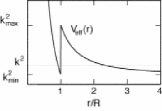
Figure 10: Effective potential picture for whispering gallery resonances of the cylinder; $k_{min}=m/(nR)$ and $k_{max}=m/R$.

At nonzero angular momentum one sees that a metastable well is formed within the dielectric. The electric field inside is separated from the propagating field outside by a tunnel barrier, and one may expect solutions of the wave equation in which the intensity inside the well is exponentially larger than outside the well. In order to complete the formal analogy to the one-dimensional Schrödinger equation we make a substitution of variables to eliminate the first derivative term in the radial equation (277). This can be achieved by introducing a new coordinate $\xi:=\ln(kr)$; the resulting equation is

$$\left[\frac{d^{2}}{d\xi^{2}}+q^{2}(\xi)\right]\vec{E}(r)=\vec{0}\;,$$ (279)

where $q(\xi)=(n^{2}\exp(2\xi)-m^{2})^{1/2}$, and $q(\xi)$ is the effective wave vector of the rescaled problem. In order that there are any resonant solutions, $kR$ must be sufficiently large so that $q$ is real for some value of $r$ within the dielectric. The largest value of the argument of the square root within the dielectric occurs when $r=R$, so we deduce the condition

$$k_{\rm min}=\frac{m}{nR}\;.$$ (280)

On the other hand, if infinitesimally outside the dielectric where $n=1$, $q$ is real, then there is no region of exponential decay, and no sharp resonances exist. The maximum value of $k$ such that $q$ is imaginary just outside the dielectric is given by

$$k_{\rm max}=\frac{m}{R}\;.$$ (281)

Consequently, we expect narrow resonances of angular momentum $m$, broadened only by tunnelling decay (evanescent leakage), for wave vectors satisfying

$$\frac{m}{nR}<k<\frac{m}{R}$$ (282)

or equivalently

$$\frac{1}{n}<\frac{m}{nkR}<1\;.$$ (283)

We will label these metastable well states by a discrete index $\nu$ which corresponds to the number of radial nodes. If the refractive index is changed, the barrier top in Fig. 10 remains the same, but the well grows deeper so that the lowest allowed $k$ will give rise to a narrower resonance. Later we will show that essentially all of the metastable states satisfying (282) are discrete in the sense that their spacing in $k$ is larger than their decay width through the barrier. In this way they will give rise to isolated resonances in the scattering functions which are well set apart from the background.

It is worth quoting here the main features of the numerically observed resonances in plane-wave scattering off a dielectric cylinder at normal incidence, as given in Ref. [48] (but using our notation):

…their widths decrease as $m$ [angular momentum] increases for a given $\nu$ [radial node number], and their widths increase as $\nu$ increases for a given $m$. Also, as the index of refraction [$n$] is increased, the positions of the resonances shift to lower $kR$, and their widths become narrower. Resonances having relatively narrow widths occur in the range $x$ to $n\,x$.

All of the above phenomena can already be understood qualitatively by inspecting the effective potential picture.

The inequality (283) can be brought into a very suggestive form which can be justified by considering the short-wavelength limit in the WKB approximation [54]:

$$\sin\chi:=\frac{m}{nkR}\;,$$ (284)

then (283) leads to

$$\frac{1}{n}<sin\chi<1\;.$$ (285)

The right inequality is trivial, but the left relation is precisely the condition for total internal reflection which must be satisfied by the angle of incidence $\chi$ on the high-index side at an interface to air, cf. (275). At this point we have provided no reason why $\chi$, as defined here, should be the classical angle of incidence. Let us try a non-rigorous argument: If we interpret the ray trajectories as classical particles with momentum $\hbar(nk)$ inside the resonator, and angular momentum $L=\hbar m$, then the classical relation between angular and linear momentum would imply $\vec{L}=\vec{r}\times\vec{p}\leadsto L=R\,(\hbar nk)\,\sin\chi\leadsto m=R\,nk\,\sin\chi$, where $\sin\chi$ arises from the vector product of linear momentum and radius vector ${\bf r}$, which in turn has magnitude $R$ at every reflection from the boundary. At such a reflection, $\chi$ is then just the angle of incidence.

The introduction of $\hbar$ into the present optical context is somewhat arbitrary. The question is, does the optical field in the cavity truly acquire angular momentum. We know that photons, as massless fundamental particles, carry a unit spin angular momentum, but no orbital angular momentum in the physical sense. Therefore, when we refer to $m$ as an angular momentum quantum number, we invoke a formal analogy that arises between the mathematical structure of bound photonic states and bound quantum systems: There are, in our case, two degrees of freedom which are associated with a finite region of space, giving rise to a discrete frequency spectrum. The modes are then labeled by as many discrete indices, or “quantum” numbers as there are confined degrees of freedom. For a rotationally symmetric problem, the indices, or quantum numbers, are simply the number of radial and azimuthal nodes of the wave function. The azimuthal quantum number is what we call $m$. Its relation to the angle of incidence is rigorously derivable from the eikonal (or WKB) limit [54].

There is an additional complication to this argument if the cavity is not closed. Due to the openness of the system, it is then not clear how to define the photons in a resonant mode. However, the cavity can approach the closed limit as $n\to\infty$. Before we discuss this problem, we will elucidate the concept of modes in the leaky cavity setting, where discrete resonances appear but have a finite width in $k$. We will return to this issue under the heading of quasibound states in section 6.4.

For this moment let us nevertheless dwell on (285), which we can use to interpret some results. For example, it indicates that states at the bottom of the well correspond to a ray motion tangential to the boundary, whereas states at the top correspond to rays colliding with the boundary at exactly the critical angle. As next we turn to a more detailed discussion of the actual wave solutions for the dielectric cylinder where the incident wave propagation is normal to the axis.

6.3.2 Matching conditions for TM polarization

Our general considerations so far have not addressed the boundary conditions at the interface between dielectric and vacuum (or air) – conditions which also depend on the polarization of $\vec{E}$. The arguments given above for the existence of narrow resonances are, however, independent of the boundary conditions, because we rely only on the fact that a tunnel barrier is formed where the field decays. Thus there should exist resonances corresponding to two different polarization states. Henceforth we will focus on the transverse magnetic polarization for which the boundary conditions lead to the simplest matching conditions for the electric field inside and outside the dielectric. For this polarization state we assume an incident plane wave of the form $\vec{E}=E(x,y)\,\vec{e}_{z}$, where the unit vector $\vec{e}_{z}$ points parallel to the cylinder axis (and hence the magnetic field is transverse to the cylinder axis). From now on we will focus on the scalar function $E(x,y)=E(r,\phi)$ which is the amplitude of the electric field in $z$-direction. Since a pure dielectric is an insulator, there is no current flowing on its surface in response to the incident field and $\vec{H}$ is continuous everywhere (neglecting any variation in the magnetic permeability). From (268), we derive the azimuthal component of the magnetic field, which in polar coordinates has the form

$$H_{\phi}=\frac{\mbox{i}}{k}\left[\nabla\times E\vec{e}_{z}\right]_{\phi}=-\frac{\mbox{i}}{k}\,\frac{\partial E}{\partial r}\;.$$ (286)

Therefore the radial derivative of $E(r,\phi)$ is continuous at the dielectric surface. Since the tangential component of $E$ is always continuous at such an interface, we arrive at the simple matching conditions that both $E$ and ${\partial E}/\partial r$ are continuous at the cylinder surface. TE polarization ($\vec{H}$ along $\vec{e}_{z}$) does not result in these familiar requirements [46, 47], however one can still obtain a scalar wave equation, which can be treated with a generalization of the methods used below. Most conveniently, one writes the wave equation for the magnetic field $H$, which is again continuous, but exhibits a jump of magnitude $n^{2}$ in the normal derivative at the interface. The effective potential picture with purely tunneling escape for the whispering gallery modes remains unchanged by this, since our arguments above did not involve polarization. Note that for TE polarization the electric field is in the plane of incidence. Transmission out of the dielectric becomes unity at the Brewster angle which neglecting the finite curvature of the interface is given by

$$\sin\chi_{B}=\frac{1}{\sqrt{1+n^{2}}}\;.$$ (287)

The whispering gallery mode criterion $\sin\chi>1/n$ is clearly not modified by this effect since $\sin\chi_{B}<1/n$.

An important point is that the same matching conditions remain valid even when the cross section of the cylinder is non-circular, because for TM polarization $\vec{E}$ remains tangential to the surface. As long as we consider only convex surfaces, the continuity of $\partial E/\partial r$ in polar coordinates implies the continuity of the normal derivative of $E$. These boundary conditions are identical to those for quantum scattering from a potential well. Hence, we are allowed to use the terms familiar from quantum theory, such as tunneling, as we did in the previous sections. However, as was already noted with (276), it should be kept in mind that the analogy is incomplete, because the dispersion relation in quantum mechanics is $\omega=\hbar\,k^{2}/(2m)$ and not $\omega=n\,c\,k$ as in optics. The results presented here can therefore not be obtained by simply copying known quantum mechanical calculations. An important difference between the quantum and optical wave equations can be read off (278), where the effective potential well is seen to become progressively deeper with increasing $k$. As a consequence, above barrier reflection remains significant even for large $k$, whereas it would become negligible in an attractive circular quantum well at high energies. This effect is just the well known classical Fresnel reflection at a dielectric interface, which independently of the wavelength has the value $R=(1-n)^{2}/(1+n)^{2}$ at normal incidence, i.e. $\sin\chi=m/(nkR)\to 0$.

6.3.3 Resonances in elastic scattering

The wave equation for TM (or TE) polarization as defined above is of the scalar form

$$\nabla^{2}\psi+n^{2}k^{2}\,\psi=0\;,$$ (288)

where $\psi$ denotes the electric field for the TM case, and the refractive index $n$ is a constant different from $1$ inside the dielectric. The wavenumber $k$ is not position dependent because it enters the problem simply through the definition $\omega=c\,k$ for the harmonic time dependence. All the scattering functions for the elastic scattering of light (i.e. scattering at the fixed frequency $\omega$) by a dielectric cylinder can be calculated if we know the scattering states

$$E_{m}(r)=\begin{cases}A_{m}\,J_{m}(nkr)&(r<R)\\ H^{(2)}_{m}(kr)+S_{m}\,H^{(1)}_{m}(kr)&(r>R),\end{cases}$$ (289)

for all $m$ ($J_{m}$ and $H_{m}$ denote the Bessel and Hankel functions, respectively). These are solutions to the radial equation(277), assuming that the refractive index is unity outside the cylinder and $n(r)=1+(n-1)\Theta(R-r)$ inside. The amplitudes $A_{m},S_{m}$ are determined by the matching conditions for $E$ and its radial derivative $E^{\prime}$,

$$A_{m}\,J_{m}(nkR) = H^{(2)}_{m}(kR)+S_{m}\,H^{(1)}_{m}(kR)$$

$$A_{m}\,nJ^{\prime}_{m}(nkR) = H^{(2)\prime}_{m}(kR)+S_{m}\,H^{(1)\prime}_{m}(kR)\;,$$ (290)

where, the primes denote differentiation. e.g. $J^{\prime}(x)=dJ/dx$. This can be solved for the scattering amplitude $S_{m}$ as a function of the size parameter $x\equiv kR$. In terms of quantum mechanical scattering theory, $S_{m}$ is a diagonal element of the scattering or S-matrix which for the rotationally invariant scatterer is diagonal in the basis of angular momentum states $m$. Using these solutions, one can for example calculate the scattering properties for an incident plane wave. A plane wave can be decomposed into a combination of Bessel functions [52] as

$${\rm e}^{-{\rm i}kx}=\sum\limits_{m=-\infty}^{\infty}(-\mbox{i})^{m}{\rm e}^{{\rm i}m\phi}J_{m}(kr).$$ (291)

This then determines the coefficients with which the partial waves (289) are superimposed to get the full solution. The conventional representation of this solution is [48]

$$E(r,\phi)=\begin{cases}\sum\limits_{m=-\infty}^{\infty}e^{im\phi}\,(-i)^{m}d_{m}\,J_{m}(nkr)&(r<R)\\ \sum\limits_{m=-\infty}^{\infty}e^{im\phi}\,(-i)^{m}\left[J_{m}(kr)-b_{m}\,H^{(1)}_{m}(kr)\right]&(r>R)\end{cases}$$ (292)

Using $J_{m}=\frac{1}{2}(H^{(1)}_{m}+H^{(2)}_{m})$ in the incoming wave, this becomes for $r>R$

$$E(r,\phi)=\frac{1}{2}\,\sum\limits_{m=-\infty}^{\infty}{\rm e}^{{\rm i}m\phi}\,(-\mbox{i})^{m}\left[H^{(2)}_{m}(kr)+(1-2\,b_{m})\,H^{(1)}_{m}(kr)\right],$$ (293)

so that we can extract the relationship between $S$- and the $b$-coefficients,

$$S_{m}=1-2\,b_{m}\;.$$ (294)

Hence the $b_{m}$ are analogous to the quantum mechanical transition matrix $T$, defined by $S=1-2\pi\mbox{i}\,T$. The S-matrix satisfies an additional condition as a consequence of flux conservation, namely [14]

$$S^{\dagger}S=1.$$ (295)

This unitarity relation also holds for deformed resonators, where $S$ is not diagonal. It provides an independent equation with which to check the accuracy of the wavefunction matching. For the circular cylinder, unitarity just implies that all $S_{m}$ have modulus one. For numerical calcultions borrowing this formalism from quantum-mechanics is therefore an added advantage.

If a plane wave is incident on the cylinder, the scattered intensity has the angular dependence [46, 47]

$$I(\phi)\propto\left|\sum\limits_{m=-\infty}^{\infty}b_{m}\,{\rm e}^{{\rm i}m\phi}\right|^{2}\;,$$ (296)

where $\phi$ is the angle with the beam. From the matching conditions (290), one finds that the expansion coefficients can be written in the form

$$b_{m} = \frac{1}{1+i\,\beta_{m}}\;,$$ (297)

$$\beta_{m} = \frac{n\,{\rm J}_{m-1}(nx)\,{\rm Y}_{m}(x)-{\rm J}_{m}(nx)\,{\rm Y}_{m-1}(x)}{n\,{\rm J}_{m-1}(nx)\,{\rm J}_{m}(x)-{\rm J}_{m}(nx)\,{\rm J}_{m-1}(x)}\;,$$ (298)

where we have used the abbreviation

$$x\equiv kR\;,$$ (299)

and the function ${\rm Y}_{m}(x)$ is the Bessel function of the second kind. This provides an explicit formula for the scattering intensity $I(\phi)$, an example of which is plotted in Fig. 11. As is seen in the figure, the scattered intensity shows rapid resonant variations. The resonances are not simply Lorentzian peaks, but are of the Fano shape [56] with varying values of the Fano asymmetry parameter. This asymmetric shape is due to interference between the nonresonant scattered waves and the resonant scattering. As long as the resonance is sufficiently isolated the resonance widths can be extracted by fitting a Lorentzian to the Fano function. It can immediately be observed that the resonances have widely varying widths corresponding to how close they are to the top of the barrier in the effective potential well.

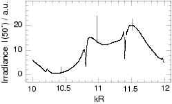
Figure 11: Irradiance $I$ which is scattered off a circular cylinder with refractive index $n=2$ at $\phi=50^{\circ}$ with respect to the direction of the incoming wave which is assumed to be plane and TM polarized.

The decomposition (297) is analogous to the case of a scattering sphere [53], and in the same way one observes that intensity maxima occur near the value of $k$ at which one of the $b_{m}$ has a maximum (if there is no interference with other nonresonant waves then it will be at exactly that value of $k$). This in turn occurs when $\beta_{m}=0$. Thus, we set (298) to zero and obtain an implicit equation for the resonance positions $x=kR$ in each angular momentum channel $m$:

$$n\,{\rm J}_{m-1}(nx)\,{\rm Y}_{m}(x)={\rm J}_{m}(nx)\,{\rm Y}_{m-1}(x).$$ (300)

It should be noted that the denominator of (297) is nonzero only for the regime of below barrier resonances, $x<$. Otherwise, additional resonances arise whenever $\beta_{m}$ becomes infinite, i.e. when

$$n\,{\rm J}_{m-1}(nx)\,{\rm J}_{m}(x)={\rm J}_{m}(nx)\,{\rm J}_{m-1}(x).$$ (301)

Above-barrier resonances thus occur if either (300) or (301) is satisfied. Yet, these resonances will typically be so broad that they do not give rise to isolated peaks in the scattering functions.

6.3.4 Quasibound states at complex wavenumber

Having obtained the condition for when a resonance is excited in elastic scattering, we now turn to a complementary approach in which no incident wave is present. Resonances can also be excited without any incoming wave at that frequency, e.g. if the light is generated inside, such as in a laser. Also the specific lineshape of a resonance in elastic scattering depends on the nature of the incident wave and is not a property of the scatterer alone. It is thus useful and important to consider an alternative definition of the resonant state which is independent of the manner of its excitation. We will first introduce the concept of the quasibound state. We will discuss this concept using the example of the dielectric cylinder we have have considered above, and then turn to the more general significance of such states.

Solutions of the wave equation with no incoming wave are termed quasibound states (or in the recent literature on resonances of dielectric spheres, quasinormal modes [57], hinting at the fact that they are not an orthonormal set in the usual sense). Due to the unitarity of the $S$-matrix for real $k$, there can be no such solutions for real values of $k$. Instead quasibound states are directly connected with the complex poles of the $S$-matrix (or in our simple case the matrix element $S_{m}$), the real part of $k$ giving the resonance frequency, and the imaginary part giving the resonance width. This is because the condition for having a solution to the matching equations with no incoming wave is just the condition for a pole of the $S$-matrix [58]: If in (289) we give the incoming wave ($H^{(2)}_{m}$ an arbitrary amplitude $A_{i}$, then the outgoing wave will have amplitude

$$A_{o}=S_{m}\,A_{i}\;.$$ (302)

If we now set $A_{i}\to 0$, there can be a finite outgoing radiation if at the same time $S_{m}$ has a divergence, requiring us to tune $k$ to the complex value where $S_{m}$ has a pole.

Thus the complex wavenumber of the quasi-bound state is determined by

$${\tilde{E}}_{m}(r)=\begin{cases}A_{m}\,J_{m}(nkr)&(r<R)\\ {\tilde{S}}_{m}\,H^{(1)}_{m}(kr)&(r>R)\;,\end{cases}$$ (303)

and the accompanying condition for continuity of the derivatives. These matching conditions for $\tilde{E}$ can be satisfied only for a discrete set of complex $k$ at which there exists a nontrivial solution to the homogenous part of the linear system (290). The latter occurs only at the zeroes of the determinant

$$D=\left|\begin{array}[]{cc}J_{m}(nkR)&-H^{(1)}_{m}(kR)\\ nJ^{\prime}_{m}(nkR)&-H^{(1)\prime}_{m}(kR)\end{array}\right|\;,$$ (304)

which leads to

$$nJ^{\prime}_{m}(nkR)\,H^{(1)}_{m}(kR)=J_{m}(nkR)\,H^{(1)\prime}_{m}(kR)\;.$$ (305)

Using the recursion relations for the Bessel functions to eliminate the derivatives, we obtain the resonance condition

$$n\left[J_{m-1}(nkR)-\frac{m}{nkR}J_{m}(nkR)\right]\,H^{(1)}_{m}(kR)$$

$$=J_{m}(nkR)\,\left[H^{(1)}_{m-1}(kR)-\frac{m}{kR}H^{(1)}_{m}(kR)\right]$$

$$\Rightarrow nJ_{m-1}(nkR)\,H^{(1)}_{m}(kR)=J_{m}(nkR)\,H^{(1)}_{m-1}(kR)\;.$$ (307)

This can be solved numerically to find the real and imaginary parts of $kR$ at which a metastable state occurs. Equation (307) is a complex equation for a complex variable. If we restrict $kR$ to be real, then the real and imaginary parts of the equation are precisely (300) and (301) which we obtained for the scattering resonances. This shows the direct relationship between the quasibound states and the scattering resonances: For real $kR$, (307) cannot be exactly fulfilled, but the closest one can get to satisfying it with real $kR$ is given by the scattering resonance conditions.

The exact results obtained numerically for the real parts of the quasibound state wavevectors are summarized in Fig. 12. For each $m$, there exists an infinite sequence of discrete points in this grid, corresponding to an increasing number of radial nodes in the effective potential well. The quasibound states are hence labeled by angular momentum and radial quantum numbers (which we call $m$ and $\nu$), as in the closed circle. We have drawn in Fig. 12 a line of slope $m/kR=1$ corresponding to the condition $\sin\chi=\frac{1}{n}$; resonances to the right of that line are true whispering gallery modes and we expect their widths to be much less than the resonance spacing, with the narrowest resonances corresonding to the points with the largest distance from this line.

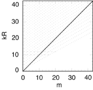
Figure 12: Resonance positions in the circle of refractive index $n=2$ with TM polarization for the lowest $44$ angular momentum numbers $m$. Each dot corresponds to one resonance, and the solid line $kR=m$ represents the dividing line between broad and narrow resonances, with narrow widths expected below it. The horizontal dashed lines enclose a $kR$ interval in which we count a total of $9$ resonances below the critical line. Compare this observation with the scattered intensity in Fig. 11. The three narrowest resonances there correspond to the three lowest $kR$ points at $m=17,\,18,\,19$. The closer the points are to the critical line, the broader the resonances get.

Note that the spacing in $k$ of resonances for a given value of $m$ is roughly constant above the line $m/kR=1$, whereas the spacing of resonances below the line increases and hence is not independent of $kR$ for a given $m$. The latter are the whispering gallery mode resonances of primary interest to us.

The uniform spacing of the above barrier resonances can be demonstrated by using the large argument expansions of the Bessel functions in (307). This is justified at large enough size parameter $nkR\gg m$, noting that $nkR>m$ always holds. One obtains

$$n\cos\left(nkR-\frac{\pi}{2}m-\frac{3\pi}{4}\right)\,H_{m}^{(1)}(kR)$$ (308)

$$= \cos\left(nkR-\frac{\pi}{2}m-\frac{\pi}{4}\right)\,H_{m-1}^{(1)}(kR).$$

Noting that $\cos(\alpha-\pi/2)=\sin\alpha$, this simplifies to

$$\tan\left(nkR-\frac{\pi}{2}m-\frac{\pi}{4}\right)=\frac{1}{n}\;\frac{H_{m}^{(1)}(kR)}{H_{m-1}^{(1)}(kR)}\;.$$ (309)

An important limiting case is $n\to\infty$, for which the large argument expansion always applies if $m$ and $kR$ are fixed. Then the righthand side becomes negligible, so that the resonance position is given by

$$kR=\frac{\pi}{n}\left[\frac{m}{2}+\nu+\frac{1}{4}\right]\>,$$ (310)

where the nonnegative integer $\nu$ is the radial quantum number. This is just the limit of a closed system with Neumann boundary conditions, $J^{\prime}_{m}(kR)=0$, in the limit $nkR\gg m$, and it clearly leads to a purely real $kR$, i.e. to truly bound states.

On the other hand large $n$ is not always necessary to get an approximate result: one obtains the same expression for the resonance position independently of $n$, provided the quotient of the Hankel functions is purely imaginary. This is precisely the case for above-barrier resonances, where $kR>m$, and hence we can use the large argument expansion for the Hankel functions, too. The righthand side in (309) then becomes equal to $-\mbox{i}/n$, and one can solve exactly for

$$nkR=\frac{\pi}{2}m+\frac{\pi}{4}+\frac{i}{2}\left[\ln\frac{1-1/n}{1+1/n}-i2\pi\nu\right].$$ (311)

Thus the real and imaginary parts of $kR=x+iy$ can be given analytically in the limit $kR>m$:

$$x = \frac{\pi}{n}\left[\frac{m}{2}+\nu+\frac{1}{4}\right]$$ (312)

$$y = \frac{1}{2n}\ln\frac{1-1/n}{1+1/n}\;.$$ (313)

Since the righthand side in (309) has no real part when $kR\ll m$, it does not affect the condition for the real part of $kR$. The approximations made here are thus valid either for large $n$ or for above barrier resonances.

Of greatest interest to us, however, are the long-lived resonances with $kR>m$. For this case, the ratio of Hankel functions will acquire an $m$- and $k$-dependent real and imaginary part, which will emerge in both resonance positions and widths. Approximate explicit expressions for resonance widths and positions can be obtained, but are not generally valid for the entire range of interesting parameters $n$, $kR$, $m$ [55] – therefore, we can for now be content with the simple limiting cases considered here. They are already of practical use because a numerical solution of the implicit equation (307) for the real and imaginary part of $k$ at given $m$ and $n$ is made more efficient by using the approximate resonance positions from (312) as an initial guess in finding the roots of (307).

6.4 Quasibound states in lasing and fluorescence

The previous considerations have brought us to the quasibound state concept via the resonances in elastic light scattering. Even if we allow the cross section of our dielectric cylinder to be deformed, TE and TM polarization can still be decoupled (see the remarks in section 6.3.2), provided we continue to restrict ourselves to propagation normal to the cylinder axis. After we clarified the role a complex wavenumber $k$ can play in the original wave equation, we deduce a rather general statement about quasibound states. To arrive at the time-independent wave equation (273), we assumed a monochromatic time variation ${\rm e}^{-{\rm i}ckt}$, with $k=\omega/c$ according to (270). With the quasibound state boundary condition (no incoming wave), this same wave equation admits solutions only at discrete complex $k=\omega/c-\mbox{i}\,\gamma/c$, where we have split the frequency into its real and imaginay part. Returning to the ansatz for the time dependence, this implies that the quasibound state decays in time as $\exp[-\mbox{i}\omega\,t-\gamma\,t]$.

This decay is of course a consequence that the system is open and radiates energy away to infinity. Consequently, the corresponding “radiation boundary condition” is composed only of outgoing waves which are present far away from the cavity. This is the type of boundary condition that occurs in many emission problems, in particular in lasing. To see how these “leaky modes”, which we found in the treatment of the passive cavity, arise in lasing, we have to take a new point of view: Consider a scalar wave equation of the form

$$\nabla^{2}\psi+{\tilde{n}}^{2}k^{2}\,\psi=0,$$ (314)

as it arises for each of the coupled polarization directions in the cylinder. This is similar to (273) where we made the ansatz of a steady-state time dependence with real $k$. If we do indeed require $k$ to be real, then in order to find a solution satisfying the radiation condition, we permit the refractive index to be complex inside the resonator, which we denote by $\tilde{n}=n-\mbox{i}\,n^{\prime}$, where $n$ is the real part. The imaginary part allows to introduce an amplifying medium. Consider the simple example of a plane wave $\exp[\mbox{i}\tilde{n}kx]$ which will clearly grow with $x$ in the direction of propagation. This is the “energy source”, but note that the detailed mechanism of this energy production, for example the pumping mechanism, is not defined in this way. Nevertheless, outside the cavity, we again assume air with $\tilde{n}=1$ with matching conditions that are appropriate for the given polarization. Finally, let us assume TM polarization as before in the scattering problem. The solutions for the exterior and interior field are $\psi_{\rm ext}$ and $\psi_{\rm int}$.

Let us now recast (314) as

$$\nabla^{2}\psi+n^{2}\tilde{k}^{2}\,\psi=0\;,$$ (315)

where $n$ is the real part of $\tilde{n}$ as defined above, and $\tilde{k}=k-\mbox{i}\,k\,n^{\prime}/n$ is the complex wavenumber inside the cavity, which reduces to $\tilde{k}=k$ outside. This recast equation is almost of the form of (288), except that $k$ has different values inside and outside the cavity. If instead, we also had $\tilde{k}=k-\mbox{i}\,k\,n^{\prime}/n$ outside, the solutions of (315) were exactly the quasibound states of the passive resonator (i.e. solutions of the Helmholtz equation at complex $k$) if the deacy rate was defined as as

$$\gamma=ck\,n^{\prime}/n.$$ (316)

We now may argue that adding or dropping the imaginary part of $\tilde{k}$ outside the resonator makes only a small difference if $\gamma$ is small: In fact, as can be checked (cf. [55]) by inspecting the large-argument asymptotics of the Hankel function $H^{(2)}$, the field of a quasibound state at distances larger than $\approx c/(2\gamma)$ from the cavity grows exponentially due to retardation, but within this physical range $\psi_{\rm ext}$ vanishes as $\gamma\to 0$. Therefore one can write $\psi_{\rm ext}({\bf r})\approx\gamma\zeta({\bf r})$. If we expand $\psi_{\rm int}(\gamma)$ and $\zeta(\gamma)$ in a Taylor series in $\gamma$, then to linear order the $\gamma$-dependence of $\zeta$, but not that of $\psi_{\rm int}$, can be dropped in the full solution. Therefore, the stationary state of the active medium described by (314)) or (315), as well as the metastable decaying state obtained by replacing the real valued outside wavenumber $k$ by $k-\mbox{i}\,k\,n^{\prime}/n$ are identical to first order in $\gamma$ within an area of order $\gamma^{-2}$.

In conclusion, we have seen that long-lived quasibound states appear not only as resonances in elastic light scattering but also as stationary states in emission problems at low pump rate (characterized by $\gamma=ck\,n^{\prime}/n$). When asking for the intrinsic properties of such long-lived states, it is often a good starting point to consider first the limiting case of no losses, i.e. the closed cavity. In the next section, we discuss the familiar concept of Gaussian beams as freely propagating waves, and how they can be used to describe resonator modes. Although since the work of Fox and Lee [62] this is the standard approach to describe laser resonators [28], this approach has some severe limitations for microresonators.

6.5 Paraxial approximation and the parabolic equation

In free space, the spectrum of electromagnetic waves is not only continuous but highly degenerate, as can be seen, for example, by choosing plane-wave solutions of the Helmholtz equation and noting that at each frequency an infinite number of propagation directions can be chosen. There exists a class of approximate free space solutions of the Helmholtz equation, the Gaussian beams. Gaussian beams are obtained by introducing the slowly-varying envelope approximation in the wave equation. This is a special case of a frequently encountered approximation which is labelled with different names, for example adiabatic approximation, paraxial approximation, or Born-Oppenheimer approximation. In the theory of partial differential equations one also finds the name “parabolic-equation” method, because the main step is to neglect the second derivative of a slowly-varying “envelope” function, which results in an equation of the type of the time-dependent Schrödinger equation for the latter. In optics, this approximation leads to the Fresnel propagator describing diffraction in the limit of small angles with the optical axis.

6.5.1 Gaussian beams and the short-wavelength limit

Gaussian beams play a prominent role in traditional laser optics, because they arise naturally as solutions in parallel-mirror resonator structures, and they also represent diffraction-limited propagation. However, they are not in general acceptable functions to describe the modes of a microcavity. In contrast to free space, it is not even clear a priori how to define the equivalent of the paraxial condition in a general microresonator structure, such as for example a circular disk. To clarify this point, we will discuss the paraxial approximation as next.

Behind the paraxial approximation is the picture of a “light beam” propagating in $z$-direction. Let us assume that the beam is described by the envelope function

$$\psi(x,y,z)\equiv u(x,y;z)\,{\rm e}^{{\rm i}kz}$$ (317)

which we insert into the Helmholtz equation

$$\nabla^{2}\psi+k^{2}\psi=0\;.$$ (318)

As aresult we obtain

$$u_{xx}+u_{yy}+u_{zz}+2\mbox{i}\,ku_{z}=0\;.$$ (319)

With this step we have formally reduced the wavenumber exponent by one, without loss of information.

In the paraxial approximation we take (319), but neglect the second order derivative $u_{zz}\equiv\partial^{2}u/\partial z^{2}$. In what situation is this appropriate? The name “paraxial” comes from a comparison between length scales over which wave solution extends along $z$ and in the transverse directions, respectively. Let $L$ be the relevant length in the $z$ direction. Now let us introduce rescaled coordinates which measure the transverse space in dimensionless form as [59]

$$x^{\prime}=x\,\sqrt{k/L},\quad y^{\prime}=y\,\sqrt{k/L},\;,$$ (320)

while for the longitudinal dimension we set

$$z^{\prime}=z/L\;.$$ (321)

With this (319) appears as

$$\frac{k}{L}\left(u_{x^{\prime}x^{\prime}}+u_{y^{\prime}y^{\prime}}\right)+\frac{1}{L^{2}}\,u_{z^{\prime}z^{\prime}}+2ik\,\frac{1}{L}\,u_{z^{\prime}}=0\;.$$ (322)

With multiplication by $L/k$ we obtain

$$u_{x^{\prime}x^{\prime}}+u_{y^{\prime}y^{\prime}}+\frac{1}{kL}\,u_{z^{\prime}z^{\prime}}+2iu_{z^{\prime}}=0\;.$$ (323)

Thus, the second order $z^{\prime}$ derivative can be neglected, if $1/kL\ll 1$. In cases in which this is fulfilled the paraxial approximation is appropriate.

As $1/kL=\lambda/2\pi L\ll 1$ implies $\lambda\ll L$, the paraxial approximation corresponds in fact to a short-wavelength approximation. The approximation consists in the assumption that the envelope $u$ is slowly-varying compared to the wave fronts along $z$. The resulting equation in the original coordinates reads as

$$-\left(\frac{\partial^{2}}{\partial x^{2}}+\frac{\partial^{2}}{\partial y^{2}}\right)u=2\mbox{i}k\frac{\partial u}{\partial z}\;.$$ (324)

This equation is mathematically of a fundamentally different type than the Helmholtz equation: whereas the former is an elliptic partial differential equation, the latter is parabolic. The difference is that solutions of an elliptic equation are determined by solving a boundary-value problem, while solutions of (324) are specified by initial conditions along a line $z=z_{0}$, for example. If we try to impose boundary conditions on (324) by specifying the values of $u$ on a closed surface in $x,\,y,\,z$ (e.g. a microresonator), there will in general be no solution for any $k$, whereas the original eigenvalue problem (318) always exhibits solutions satisfying the boundary conditions for a discrete set of $k$-values. This well-known consequence of the theory of characteristcs [61] by which second-order partial differential equations are classified explains why paraxial approximations in general do not allow to find all the modes of a resonator.

Let us put it in other words: Equation (324) is formally analogous to the time-dependent Schrödinger equation in which we substitute $z\leftrightarrow t$ and $k\leftrightarrow m/\hbar$. We know that this equation uniquely determines the time evolution of any initial wave packet prepared at time $t=t_{0}$. This corresponds to specifying the solution of (324) at some $z=z_{0}$. Clearly, if in addition to the initial condition we also want to impose an arbitrary “final distribution” of $u$ at some other time $t=t_{1}$, then, in general, a contradiction will arise to the unique time evolution. Only for special choices of initial distributions can the final condition be met. Boundary conditions on a closed surface in the “spacetime” spanned by $x,\,y,\,z$ are therefore not generally consistent with (324). Now, based on this parabolic equation how can we find the modes of a closed resonator?

6.6 Gaussian beams in free space

There are various schemes by which this can be accomplished for some subset of modes, and the vast majority of conventional resonator calculations in optics are based on such methods [28]. In order to discuss these approaches and their limitations for microcavities, we first recall how the propagation along $z$ (or the “time evolution”) can be expressed in terms of the retarded Green function $G$:

$$u(x^{\prime},y^{\prime};z^{\prime})=\int G(x^{\prime},y^{\prime},z^{\prime};\,x,y,z_{0})\,u(x,y;z_{0})\,dx\,dy\;.$$ (325)

The Green function of the free particle time dependent Schrödinger equation, also called its propagator [60], is well known from quantum mechanics [14] as well as from the theory of thermal conduction [61] (where it appears with an imaginary time scale):

$$G(\vec{r}\,^{\prime},t^{\prime};\,\vec{r},t)=\left[\frac{k}{2\pi\,\mbox{i}\,(t^{\prime}-t)}\right]^{d/2}\,{\rm e}^{{\rm i}k(\vec{r}\,^{\prime}-\vec{r})^{2}/2(t^{\prime}-t)}\quad(k\equiv m/\hbar).$$ (326)

Here, $d=1,2,3$ is the number of spatial dimensions. This result reminds us of another important feature of the parabolic equation: The above function describes how a wavepacket localized at a single point $\vec{r}$ at time $t$ spreads with time. Such pulse spreading is completely absent in the time dependent Green function of Maxwell’s wave equation, $(\nabla^{2}-\partial^{2}/\partial(ct)^{2})\,u=0$, where the time dependence is simply given by the effect of retardation, $G\propto\delta(t^{\prime}-t-\sqrt{x^{2}+y^{2}+z^{2}}/c)$ (in three dimensions).

The discussion in quantum mechanics textbooks usually applies to three space dimensions ($d=3$). However, we require the analogous objects for the case of two spatial dimensions ($d=2$) – in the paraxial approximation, $z$ takes the role of a time parameter and hence leaves only $x$ and $y$ as spatial coordinates. The reduced dimensionality introduces different prefactors in Green’s function but leaves the basic implications of the paraxial approximation (including pulse spreading) unchanged. With $d=2$, (325) describes the transverse profile of a paraxial beam, as it propagates along the $z$ axis. The equation is identical to the Fresnel wave propagation formula [63] for the field $\psi$, if we use the definition of $u$ in (317).

The Green function in 325, alias the Fresnel propagation kernel, defines an integral equation for the transverse mode functions $u(x,y)$, which is a frequent starting point for determining resonator modes in the paraxial approximation. Before we turn to the problem of resonator modes, it is useful to consider first the eigenfunctions of (325) in free space which are called Gaussian beams. The derivation of the fundamental Gaussian beam profile follows the analogy between (324) and the time dependent Shrödinger equation. An important solution is the minumum-uncertainty wavepacket,

$$u(x,z)=\frac{1}{(2\pi)^{1/4}}\,\frac{1}{\sqrt{\sigma+\frac{{\rm i}\,z}{2k\sigma}}}\,\exp\left[-\frac{x^{2}}{4\sigma^{2}+2\mbox{i}z/k}\right],$$ (327)

where $\sigma$ is the width of the wavepacket in $x$ direction at “time” $z=0$. An analogous form can be found for the other transverse direction, $y$, and the full wave function requires taking the product of both profiles. This separability is a consequence of the fact that we have imposed no boundary conditions on the free-space propagation. We can therefore restrict ourselves without loss of generality to wave functions that depend only on one transverse coordinate ($x$) for now.

Note that (327) is a special minimum uncertainty wavepacket with zero average $x$-momentum. By the uncertainty relation, $\sigma$ is related to to the spread in wavenumber $k_{x}$ through

$$\sigma\,\Delta k_{x}=1/2\;.$$ (328)

The wavepacket therefore has a nonzero width $\Delta k_{x}$ in Fourier space, which will lead to divergence as a function of “time” $z$. By decomposing prefactor and exponent into their real and imaginary parts, it is straightforward to show that (327) describes a standard Gaussian beam [64], if we reinstate the definition $\psi=u\,\exp(\mbox{i}kz)$ and interpret $2\,\sigma$ as the minumum spot size at $z=0$. The divergence, or angular beam spread, is given by

$$\theta=\arctan\left(\frac{1}{k\,\sigma}\right)\;.$$ (329)

It must be emphasized that the Gaussian beam is not an exact solution of the free-space Helmholtz equation (318), but becomes exact only in the paraxial limit. The beam spreading is, however, not an artefact of this parabolic equation method. It correctly describes the conjugate relation between spot size and transverse wavenumber which is a consequence of diffraction.

6.7 Gauss-Hermite beams

The spot size $2\,\sigma$ is a parameter at our disposal, by which we can determine the relative uncertainties in position and momentum according to (328). This freedom is important when one attempts to construct approximate resonator modes by properly adjusting Gaussian beams, as we will see below. Further generalizations of the fundamental Gaussian beam are possible in free space, by allowing the transverse amplitude to vary. An important special case are the Gauss-Hermite beams which are constructed as follows. If we set $z=0$ in (327), then the resulting instantaneous Gaussian

$$u_{0}(x)=\frac{1}{(2\pi)^{1/4}}\,\frac{1}{\sqrt{\sigma}}\,e^{-x^{2}/4\sigma^{2}}$$ (330)

can be formally interpreted as the ground state wavefunction of a one dimensional harmonic oscillator,

$$-\frac{\hbar^{2}}{2m}\;\frac{d^{2}u_{n}}{dx^{2}}+\frac{1}{2}\,m\omega^{2}\,u_{n}=E_{n}\,u_{n},$$ (331)

in which formally identify the oscillator length with the beam spot size,

$$\ell=\sqrt{\frac{\hbar}{m\omega}}\equiv\sqrt{2}\,\sigma\;.$$ (332)

Higher order eigenfunctions can be generated by acting on $u_{0}$ with the formal creation operator

$$a^{\dagger}\equiv\frac{1}{\sqrt{2}}({\hat{Q}}-\mbox{i}\,{\hat{P}}),$$ (333)

where we defined the operators

$${\hat{Q}} \equiv \frac{x}{\ell}=\frac{x}{\sqrt{2}\sigma}\;,$$ (334)

$${\hat{P}} \equiv \frac{\ell}{\mbox{i}}\,\frac{d}{dx}=\frac{\sqrt{2}\sigma}{\mbox{i}}\,\frac{d}{dx}\;.$$ (335)

The solutions are products of Hermite polynomials and the Gaussian $u_{0}$. From this construction at $z=0$, however, it is not directly obvious how the beam shape changes as it propagates along $z$. To see this we will define a generalized creation operator $c^{\dagger}$ which properly describes the spreading (divergence) of the beam, and which, when applied to the $z$-dependent $u(x,z)$ of (327), generates functions which are solutions of the parabolic equation (324).

For propagation in the $x-z$ plane to which we restricted our attention, the transverse beam coordinate is $x$, whereas $z$ is the propagation direction playing the role of a time variable. Let us define the following dimensionless quantities

$$p \equiv \frac{1}{2k\sigma}\;,$$ (336)

$$q(kz) \equiv p\,kz-2\,\mbox{i}p\,(k\sigma)^{2}\;,$$

where $k$ and $\sigma$ are the parameters from (327) for which we thus obtain

$$u(kx,kz)=\frac{1}{(2\pi)^{1/4}}\,\sqrt{\frac{-\mbox{i}k}{q(kz)}}\,\exp\left[\mbox{i}p\frac{(kx)^{2}}{2\,q(kz)}\right].$$ (337)

We can now define a generalized form of the creation operator (333) as

$$c^{\dagger} \equiv p^{*}k\,x+\mbox{i}\,q^{*}\frac{\partial}{\partial(kx)}\;,$$ (338)

$$c \equiv p\,k\,x-\mbox{i}\,q\frac{\partial}{\partial(kx)}\;,$$ (339)

which in the limit $z=0$ reduces to (333) because then $q=-\mbox{i}k\sigma$. One can verify that (338) and (339) lead to the correct commutation relation $[c,c^{\dagger}]=1$, as a direct consequence of the fact that the quantities defined in (336) satisfy the relation

$$q^{*}p-q\,p^{*}=\mbox{i}$$ (340)

for all $z$. We included complex conjugation of $p$ even though it is real, in order to highlight the similarity to the quantum commutation relation between conjugate operators – and indeed, $p$ can be interpreted formally as the conjugate momentum of the complex trajectory $q(kz)$ because it satisfies the equation of motion $p=dq/d(kz)$ with dimensionless time $kz$.

For $c^{\dagger}$ generating Gauss-Hermite beams, this operator must exhibit two additional qualities which we check in the following.

• First, we verify by direct application of (339) that $c$ annihilates the fundamental beam $u(x,z)$ given in (327).

• Second, we verify that $(c^{\dagger})^{m}\,u(x,z)$ with $m=1,2\ldots$ is again a solution of the free-space parabolic equation (324).

This latter property requires that $c^{\dagger}$ commutes with the differential operator

$${\sf L}\equiv\frac{\partial^{2}}{\partial(kx)^{2}}+2\mbox{i}\frac{\partial}{\partial(kz)}$$ (341)

which in fact corresponds to (324) written in operator form. Thus, in operator notation the parabolic equation simply reads as

$${\sf L}\,u=0,$$ (342)

where we still assume that the $y$ dependence can be separated off. Using the definitions in Eqs. (338) and (336), we obtain

$$c^{\dagger}\,{\sf L}-{\sf L}\,c^{\dagger}=2\,\left(\frac{{\rm d}\,q^{*}}{{\rm d}(kz)}\,\frac{\partial}{\partial(kx)}-p^{*}\,\frac{\partial}{\partial(kx)}\right)\;,$$ (343)

where the righthand side vanishes because of the equation of motion ${\rm d}\,q^{*}/{\rm d}(kz)=p^{*}$. This result means that if $u$ is a solution with ${\sf L}\,u=0$, then $c^{\dagger}u$ is also a solution, because

$${\sf L}(c^{\dagger}u)=c^{\dagger}({\sf L}\,u)=0.$$ (344)

Thus, we have shown that the set of Gauss-Hermite beams are solutions of the free space wave equation in paraxial approximation.

6.8 Resonator modes in the parabolic equation approximation

The construction of resonator modes using the results obtained so far requires us first to identify what is meant by the $z$ axis along which the beams propagate, if the system is bounded by some surface. For simplicity, we first assume that this boundary is perfectly reflecting, what corresponds to Dirichlet boundary conditions. We can approach this situation from two logically distinct directions.

Traditionally it is assumed that the mirrors are shaped such that they precisely match the wavefronts of a Gaussian beam for some value of spot size $\sigma$ and wavenumber $k$. On the other logical side one can start with a desired field configuration for which the shape of suitable mirrors is sought. The goal is to find modes with a predefined form which is optimally adapted to a given practical problem. In contrast to the traditional approach this procedure has the form of an inverse boundary-value problem. It has been addressed in Ref. [65], and plays a role whenever beams have to be matched to a given situation.

The molecular sieve crystals on which this review focuses, as well as all other self-assembled realizations of dielectric microresonators such as aerosol or polymer droplets, pose instead a well defined boundary value problem with little or no freedom of adjusting the cavity shape. This forces us to take a different route if we wish to extend the results of the previous subsections.

The application of the parabolic equation method in the diffraction theory of resonators is presented in great detail in Ref. [59], where, however, the salient features are at times obscured by the mathematical apparatus that is necessary to treat wave propagation in three dimensions with inhomogenous refractive index. In the folloeing we do not take such complications into account, but approach the solution of the Helmholtz equation (318) with only $x$ and $z$ as variables, and Dirichlet boundary conditions on the cavity wall which in view of the situation with microresonators, we assume to be a two dimensional closed surface. The idea of this approach is that since the Gaussian beam is an approximate short wavelength solution near some $z$ axis, we can piece together a resonator mode by using Gaussian beams which follow a closed ray trajectory in the cavity. An example for such a closed orbit is shown in Fig. 13. It is a nontrivial example where a ray based mode analysis of the present type leads to accurate results [67].

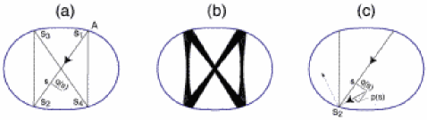
Figure 13: (a) A stable periodic orbit in an oval cavity. The path can be parametrized by the arc length $s$, i.e. the longitudinal distance along the ray from the (arbitrary) starting point A. reflections occur at lengths $s_{k}$. The stability of this bow tie shaped pattern is apparent in (b) where a ray is launched with initial position and direction slightly off the periodic path: the trajectory is nevertheless confined to the vicinity of the bow tie, performing an oscillation transverse to the trajectory in (a). The transverse deviation in position can be measured by a coordinate $q$ as shown in (c), and likewise $p$ denotes a deviation in momentum (or direction) of the initial ray. The outcome of the reflection for such a perturbed ray is shown dashed. Deviations are exaggerated for clarity.

Each straight segment of the trajectory between two successive reflections defines a $z$ axis for which the analysis of the previous subsections can be carried out. Assuming a solution of the form 337 in each segment, we determine $p$ and $q$ in a generalization of (336) such that two requirements are satisfied: The boundary conditions must be met to the accuracy of the paraxial approximation, and the full solution must be single valued (i.e. reproduce itself) after a complete round trip around the ray orbit (constructive interference condition). We retain the form given in (336), with one modification. Without modification, the minimum width of the Gaussian beam is located always at $z=0$. We can shift this location by allowing $p$ to be complex, and still maintaining the relation $q^{*}p-p\,q^{*}=\mbox{i}$ underlying the construction of the Gauss-Hermite modes. Thus we define

$$\begin{split}p&\equiv A_{1}\;,\\ q(kz)&\equiv A_{1}\,kz+A_{0}\;,\end{split}$$ (345)

where $A_{0,1}$ are complex but restricted to ${\rm Re}(A_{0}\,A_{1})=0$.

To follow the wave around the closed trajectory, we introduce a new longitudinal coordinate $s$ which measures the distance along the whole ray loop from some arbitrary starting point, say point A in Fig. 13. Then the individual reflections occur after the lengths $s_{k}$, $k=1,\ldots N$, where $N$ is the number of bounces. Furthermore, let $L$ be the length of the close path. In order for the wave function to be single-valued, the parameter $q$ governing the spreading in the transverse wave function must be periodic as a function of $s$ with period $L$, for example

$$q(s+L)=q(s)$$ (346)

for all $s$ in the interval of straight propagation we consider.

6.9 Monodromy matrix

From the boundary condition of vanishing wavefunction at the point of reflection, we get additional relationships for $p$ and $q$. Firstly, the phase of the Gaussian beams before and after reflection must exhibit a jump by $\pi$. Moreover, considering a reflection at the point $s=s_{k}$, one finds that the vector $(q,p)$ before and after reflection (at $s=s_{k}-\Delta s^{\prime}$ and $s=s_{k}+\Delta s$, respectively) must obey the equation

$$\begin{pmatrix}q(s_{k}+\Delta s)\\ p(s_{k}+\Delta s)\end{pmatrix}=M^{(k)}(\Delta s,\Delta s^{\prime})\,\begin{pmatrix}q(s_{k}-\Delta s^{\prime})\\ p(s_{k}-\Delta s^{\prime})\end{pmatrix}\;,$$ (347)

where, $M^{(k)}(\Delta s,\Delta s^{\prime})$ is a $2\times 2$ matrix which depends on the distances $\Delta s,\Delta s^{\prime}$ from the reflection point. It is called the monodromy matrix of the given reflection $k$. Its explicit form can be stated in terms of the local radius of curvature $R=R^{(}k)$ of the reflecting surface and the angle of incidence $\chi=\chi^{(}k)$ with respect to the local normal [66] as,

$$M^{(k)}(\Delta s,\Delta s^{\prime})=\begin{pmatrix}\frac{2\Delta s}{2\cos\chi}-1&\frac{(\Delta s)\,(\Delta s^{\prime})}{\alpha\cos\chi}\\ \frac{2}{R\,\cos\chi}&\frac{2\,\Delta s^{\prime}}{R\,\cos\chi}-1\end{pmatrix}\;,$$ (348)

where

$$\alpha=\left(\frac{2}{R}-\frac{\cos\chi}{\Delta s^{\prime}}-\frac{\cos\chi}{\Delta s}\right)^{-1}\;.$$ (349)

The linear matrix equation (347) holds only within the paraxial approximation, which for the reflections means that the transverse spreading at the reflection points shall be small, as measured by the real part of the exponent of (337), which is

$$\frac{1}{2}\,(kx)^{2}{\rm Im}\frac{p}{q}=\frac{1}{4}\,(kx)^{2}\lvert q\rvert^{-2},$$ (350)

where we used $q^{*}p-q\,p^{*}=\mbox{i}$. A small extent in $x$ relies therefore on $|q|/k$ being small. Away from the beam waist $\lvert q\rvert$ grows with $z$, and the growth is smaller when $k$ is large. Hence, the required limit is again that of large $k$. For details of the calculations, the reader is referred to Ref. [59].

6.10 Round trip stability of periodic orbits

As is expected from a short-wavelength aproximation, the monodromy matrix itself has a ray interpretation. Equation (347) is precisely the transformation that determines how a small deviation from the periodic ray path changes the outcome of the reflection. As noted earlier, $q$ and $p$ behave like conjugate variables, and here this fact emerges again. If we interpret formally $q$ as a cartesian coordinate transverse to the ray direction along which $s$ varies, and $p$ as the conjugate transverse momentum, then the true periodic orbit would be described by $q=p=0$ and $s=0\ldots L$. Nonvanishing $p$ and $q$ at some point $s=s_{k}-\Delta s^{\prime}$ denote transverse deviations from the periodic orbit. This leads to straight line trajectories hitting the surface slightly off the locations where the exactly periodic orbit has its reflections. The outcome of the reflection of this displaced ray is then a ray deviating from the periodic path by $q(s_{k}+\Delta s)$ in position and $p(s_{k}+\Delta s)$ in momentum. To show that these classical quantities are related by (347) in the linear way of a Taylor expansion for small deviations requires straightforward but tedious trigonometry [59, 66].

The connection between the two requirements of (346) and (347) becomes apparent, if we extend the monodromy matrix from a single reflection to include all $N$ reflections of a full round trip, and ask for the cumulated deviation of the ray, as a function of the initial displacement in position $q$ and direction (momentum) $p$. As a result we can see that in a linear approximation we simply can replace $M^{(k)}(\Delta s,\Delta s^{\prime})$ in (347) with the product $M(s)$ of the $N$ individual monodromy matrices. Assume that we start a ray at longitudinal coordinate $s$ in the first leg of the ray path, $s_{1}\leq s<s_{2}$, with deviation $q$ and $p$ from the periodic orbit [cf. Fig. 13(a)]. We are then interested in the deviation incurred along one round trip $s+L$.

The distance from $s$ to the first reflection is $\Delta s^{\prime}=s_{1}-s$, and the distance between the first and second reflection accordingly is $\Delta s=s_{2}-s_{1}$. If we denote the length between reflections at $s_{k}$ and $s_{k+1}$ by $l_{k}$, then the round-trip deviation is obtained from

$$\begin{pmatrix}q(s+L)\\ p(s+L)\end{pmatrix}=M(s)\,\begin{pmatrix}q(s)\\ p(s)\end{pmatrix}\;,$$ (351)

where for the product $M(s)$ of the $N$ individual monodromy matrices is given by

$$\begin{split}M(s)&=M^{(N)}(s-s_{N},l_{N-1})\times M^{(N-1)}(l_{N-1},l_{N-2})\\ &\quad\times\ldots\times M^{(2)}(l_{2},l_{1})\times M^{(1)}(l_{1},s_{1}-s)\;.\end{split}$$ (352)

The periodicity condition (346) requires that the vector $\vec{d}=(q(s),\,p(s))$ is an eigenvector of matrix $M(s)$. Up to now we retained the dependence on the starting coordinate $s$. However, the investigation of the eigenvalue problem becomes simpler when we eliminate this dependence. This is possible because we know how any given trajectory depends on $s$: Rays in the cavity follow straight lines, so that $q$ is a linear function of $s$, whereas $p$ is in fact a constant. (This can be compared to the similar assumption we made in (345) with $kz$ instead of $s$ as the longitudinal coordinate). For the vector $\vec{d}$ we can therefore write

$$\begin{pmatrix}q\\ p\end{pmatrix}=\begin{pmatrix}1&s\\ 0&1\end{pmatrix}\begin{pmatrix}A_{0}\\ A_{1}\end{pmatrix}=\Pi(s)\,\begin{pmatrix}A_{0}\\ A_{1}\end{pmatrix}\;,$$ (353)

where the matrix $\Pi(s)=\bigl{(}\begin{smallmatrix}1&s\\ 0&1\end{smallmatrix}\bigr{)}$ appearing here obviously has unit determinant, independently of $s$. Thus we can rewrite the periodicity condition (351) as

$$\begin{pmatrix}A_{0}\\ A_{1}\end{pmatrix}=\Pi^{-1}(s+L)\,M(s)\Pi(s)\,\begin{pmatrix}A_{0}\\ A_{1}\end{pmatrix}\;,$$ (354)

which is an eigenvalue equation. We know that the coefficient vector $\bigl{(}\begin{smallmatrix}A_{0}\\ A_{1}\end{smallmatrix}\bigr{)}$ here is by construction $s$-independent, and as a consequence, the $s$ dependence of the matrix product $E=\Pi^{-1}(s+L)\,M(s)\Pi(s)$ must cancel out. The matrix $E$ is the monodromy matrix of one whole periodic orbit, because it characterizes the propagation of small deviations along one round trip irrespective of where exactly we started. Recall, however, that we set the starting point $s$ on a specific branch of the periodic orbit. Clearly, the same arguments would apply with $s$ starting in any other branch, but then the resulting matrix equation will in general be different.

6.11 Eigenvalues of the monodromy matrix

Since $E$ is a $2\times 2$ matrix, its eigenvalues and eigenvectors are easily classified, especially since $E$ can also be shown to have unit determinant [59]. This follows from ${\rm det}(\Pi)=1$ together with classical area preservation (Liouville’s theorem) for the ray dynamics; the latter implies that also ${\rm det}(M(s))=1$. As ${\rm det}\,E=1$ the two eigenvalues $\lambda_{1,2}$ satisfy

$$\lambda_{1}\lambda_{2}=1\qquad\text{and}\qquad\lambda_{1}+\lambda_{2}={\rm Tr}(E)\equiv t$$ (355)

so that determinant and trace of $E$ fix its eigenvalues via the quadratic equation

$$\lambda_{1,2}=\frac{1}{2}\,t\pm\frac{1}{2}\sqrt{t^{2}-4}.$$ (356)

Three cases can be distinguished depending on the value of $t$:

$t>2$:

The eigenvalues are real and have different magnitude.

$t=2$:

Both eigenvalues are degenerate, $\lambda_{1}=\lambda_{2}=1$.

$t<2$:

The eigenvalues are complex and both have unit magnitude,

$$\lambda_{1,2}=\frac{1}{2}\,t\pm\frac{\mbox{i}}{2}\sqrt{4-t^{2}}=e^{\pm{\rm i}\phi}\;.$$ (357)

In this case the eigenvectors $\vec{h}_{1,2}$ are also complex conjugates of each other.

The periodic ray orbit under consideration is called linearly stable if and only if case $t<2$ holds. If this is satisfied in one branch of the path, one can show that it also holds in all others.

The difference between these cases can be appreciated if one writes a general vector $\vec{d}=(q,\,p)$ as a linear combination of the eigenvectors,

$$\vec{d}=a\,\vec{h}_{1}+b\,\vec{h}_{2}$$ (358)

and asks for its evolution under repeated application of the round trip mapping $E$. For a $\nu$-fold round trip we obtain

$$E^{\nu}\vec{d}=a\,E^{\nu}\vec{h}_{1}+b\,E^{\nu}\vec{h}_{2}=a\,\lambda_{1}^{\nu}\vec{h}_{1}+b\,\lambda_{2}^{\nu}\vec{h}_{2}=a\,e^{i\nu\phi}\vec{h}_{1}+b\,e^{-i\nu\phi}\vec{h}_{2}.$$ (359)

If $\vec{d}$ is a real vector – as it should be if it describes real ray trajectories – then $E^{\nu}\vec{d}$ is also real because $E$ is a real matrix, describing only the trigonometry of the successive reflections and the straight line ray motion in between (cf. the definitions of $\Pi$ and $M(s)$). Therefore, we know that in the last equation there can be no imaginary part, and thus nothing is changed by taking the real part. If $\vec{h}_{1}=(A_{0},\,A_{1})$, then we have

$$E^{\nu}\vec{d}=\begin{pmatrix}{\rm Re}[(a+b^{*})A_{0}]\,\cos\nu\phi-{\rm Im}[(a+b^{*})A_{0}]\,\sin\nu\phi\\ {\rm Re}[(a+b^{*})A_{1}]\,\cos\nu\phi-{\rm Im}[(a+b^{*})A_{1}]\,\sin\nu\phi\end{pmatrix}.$$ (360)

Remember that $\phi$ is a fixed eigenphase, characteristic of the given branch of the periodic orbit. If we assume for the moment that $\nu$ is not an integer but instead varies continuously, then the above equation describes an ellipse in the plane spanned by $q$ and $p$. For integer $\nu$, the trajectory simply visits discrete points on this elliptical curve every time it completes a loop. This means that the small initial deviation $\vec{d}$ from the periodic ray orbit leads to a trajectory which stays close to this original periodic path for all times. The perturbed ray only performs a small oscillation in transverse position and momentum around this original path.

In case $t>2$, the curve described by $E^{\nu}\vec{d}$ is also a conic section, but in this case a hyperbola instead of an ellipse. To see this, we go back to (360) but with real eigenvalues of the form $\lambda_{1}=1/\lambda_{2}$, cf. (355). Since for real eigenvalues the eigenvectors of the real matrix $E$ can also be chosen real, we obtain with $\xi\equiv\lambda^{\nu}$

$$E^{\nu}\vec{d}=\xi\,a\,\vec{h}_{1}+\frac{1}{\xi}\,b\,\vec{h}_{2}\;,$$ (361)

which describes a hyperbola if $\xi$ is formally allowed to vary continuously. This construction tells us that the perturbed ray deviates more and more from the periodic path with increasing $\nu$. Hence a periodic orbit whose monodromy matrix has trace $t>2$ is unstable, and for $t<2$ it is stable.

The question of stability is crucial for the applicability of the paraxial approximation in constructing resonator modes. Only if a ray orbit is stable can the paraxial approximation be justified over the whole round trip. In this case one can say that the mirror configuration as seen by the closed ray trajectory and determined by the radii of curvature $R$ at the successive reflection points acts in a focussing way. Recall that the spreading of the Gaussian beam in each ray segment is given by (350). This will be unchanged upon a round-trip if $q$ acquires only a phase, not a change in absolute value. If we determine $q$ according to (353) with $\vec{h}=(A_{0},A_{1})$ being an eigenvector of the monodromy matrix $E$, then $q(s)$ indeed changes only by the eigenvalue $e^{{\rm i}\phi}$ when after a round trip we return to the starting point $s$. This is a mere phase change provided that the orbit is stable. For unstable orbits, the eigenvalues are real and different from unity, making it impossible to recover a beam with the original spread after one period of the orbit.

6.12 Resonator eigenfrequencies in the parabolic approximation

The use of the parabolic (Gaussian beam) approximation requires that we identify the stable periodic ray orbits of the resonator at hand. This can in general be a difficult task in itself, because their number and location can depend rather sensitively on the shape of the boundary. Furthermore, it must be kept in mind that there may also be modes which are not in any way associated with stable ray orbits at all.

Assuming that we have found a set of stable orbits, we can then use the Gaussian beam solutions to construct the corresponding eigenfrequencies (within the parabolic approximation). This is done by recalling that the longitudinal coordinate $s$ along the orbit plays the role of a time-like variable due to the approximation made in (324). In order for the modal wave function to be single-valued upon a round-trip, the dependence on $s$ has to be periodic. The imposition of periodic boundary conditions introduces a longitudinal “quantum number” $m$ counting the nodes along the ray path. The equations determining the wave solutions are themselves periodic in $s$, and hence the problem is analogous to that of a periodically driven time dependent system to which Floquet’s theorem applies [59], or equivalently to Bloch’s theorem governing the band structure of spatially periodic solids. The central observation there is that the wavefunction acquires only a phase factor when a translation amounting to the periodicity interval is carried out. This is precisely the content of (357) which however holds only when a stable orbit is present.

Allowing for transverse excitations according to the harmonic oscillator ladder as described by the generalized operators (338), an additional transverse mode number $n$ labels the number of nodes in the two-dimensional Gauss-Hermite beam perpendicular to the propagation axis. The resulting quantized wavenumber is found to be [59]

$$k\,L=2\,\pi\,\left(m+\frac{N}{4}\right)+\left(n+\frac{1}{2}\right)\,\phi.$$ (362)

where $L$ is the round-trip path length of the stable orbit. $N$ is the number of reflections the ray undergoes, and this number enters here to take into account the phase shifts associated with reflection. The phase $\phi$ multiplying the transverse excitation state is the eigenphase of the monodromy matrix as defined in (357). A simple application of this formula would consist in determining the longitudinal mode spacing. The intuitively expected result is that an integer number of wavelengths must fit around the ray path.

6.13 Polygonal resonators

6.13.1 Marginally stable orbits

The stability considerations of section 6.11 provide a conceptual background helping us to understand why pathological effects can occur when the resonator is bounded by a polygon with straight sides. The example most relevant here are the hexagonal facets of a molecular sieve crystal we will present in section 7. In case of the hexagon, the boundary allows neither stable nor unstable orbits. We have precisely the marginal case $t=2$, where the round-trip monodromy matrix exhibits ${\rm Tr}(E)=2$, so that both of its eigenvalues are unity. The sides of the cavity are then neither focussing nor defocussing, and the rays deviating slightly from a closed ray path do not describe an elliptical transverse envelope as they would for a stable ray. One obtains this result by evaluating the monodromy matrix for a plane interface. The resonator modes for a straight sided cavity are thus not well approximated by Gaussian beams, as can also be seen from the simple example of a rectangular cavity, for which the solutions of the scalar wave equation are (for propagation in the $xy$ plane)

$$\psi(x,y)\propto\sin k_{x}(x-x_{0})\,\sin k_{y}(y-y_{0})$$ (363)

with suitably chosen discrete wavenumbers $k_{x,y}$ and offsets $x_{0}$, $y_{0}$.

This simple example bears no resemblance to Gaussian modes but can be solved exactly because the problem is separable in cartesian coordinates. However, not all polygonal resonator geometries permit a separation of variables. This applies in particular to hexagonal resonators – the geometry exhibited by the facets of the molecular sieves microcrystals with which microlasers were realized; cf. 7. For a polygon with precisely $120^{\circ}$ angles between adjacent sides, any ray lauched at some angle to the surface will go through only a finite number of different orientations[69], just as in the more familiar rectangular resonator where there are at most two non-parallel orientations for any ray path. In the hexagon, a ray encounters the interface with at most three different angles of incidence. Despite this apparent simplicity, there exists no orthogonal coordinate system in which the wave equation for the hexagonal cavity can be solved by separation of variables. This property is not surprising, since there is only a finite number of suitable coordinate systems available, and on the other hand there are infinitely many shapes one can think of.

6.13.2 Triangular and hexagonal resonators

Even when separability is lacking, the resonator problem may sometimes be solvable by an appropriate ansatz. An example for this is a resonator composed of three straight sides forming an equilateral triangle on which the fields are assumed to vanish (Dirichlet boundary conditions). The wave solutions in cartesian coordinates are given by [68]

$$\begin{split}\psi_{m,n}(x,y)=&\sin\left(\frac{2\pi}{3}(2m-n)\,x\right)\,\sin\left(\frac{2\pi}{\sqrt{3}}\,n\,y\right)-\\ &\sin\left(\frac{2\pi}{3}(2n-m)\,x\right)\,\sin\left(\frac{2\pi}{\sqrt{3}}\,m\,y\right)+\\ &\sin\left(\frac{-2\pi}{3}(m+n)\,x\right)\,\sin\left(\frac{2\pi}{\sqrt{3}}(m-n)\,y\right)\;.\end{split}$$ (364)

This solution is slightly more complicated than the one for the rectangular resonator of (363). In (364) there is a degenerate set of solutions ${\tilde{\psi}}_{m,n}$ of different symmetry type which are obtained by replacing $\sin$ with $\cos$ in the $x$-dependent factors. We get identical wavefunctions if we exchange the quantum numbers $m$ and $n$, replace $n$ by $m-n$, or replace $m,\,n$ by $-m,\,-n$ (simultaneous sign change); the solutions differ only in sign so that they do not represent different eigenfunctions. There are, however, true degeneracies as well. They are characterized by combinations of $m$ and $n$ giving the same wavenumber

$$k_{m,n}=\frac{4\pi}{3}\,\sqrt{m^{2}+n^{2}-m\,n}\;.$$ (365)

Since any linear combination of eigenfunctions with the same $k$ is also an eigenfunction, there is a considerable ambiguity in the spatial distribution of the wave function whenever there are degeneracies. For example, for any given $m,\,n$ we can form the superposition

$$\Psi_{m,n}=\psi_{m,n}+\mbox{i}\,{\tilde{\psi}}_{m,n}\;.$$ (366)

Shown in Fig. 14 are the three functions $\psi_{m,n}$, ${\tilde{\psi}}_{m,n}$ and $\Psi_{m,n}$ for the particular case $m=14,\,n=21$.

Figure 14: In the equilateral triangle with Dirichlet boundary conditions, degenerate wave functions (a) and (b) with $m=14,\,n=21$ are superimposed according to (366) to obtain a completely different spatial intensity pattern (c). Plotted is the absolute square of the wave function in a grayscale representation with black as the highest intensity.

The wavefunction shown in Fig. 14 (c) has nodal lines along the edges of a set of smaller triangles inscribed into the original one. The self similarity exhibited by this solution bears an intriguing resemblance to the intensity patterns recently reported in unstable laser resontors with a mirror in the shape of an equilateral triangle [70]. Although further investigations of this emerging field of open, unstable resonators are needed, it seems possible that the transverse mode structure observed in the above laser experiment is given by a two dimensional wave equation with solutions similar to the ones shown in Fig. 14. The particular linear combinations appearing in any given experimental realization can be a result of the measurement setup or perturbations that lift the degeneracies. In particular, complex-valued superpositions as given by (366) become relevant in open resonators such as those in Ref. [70]. Whereas for a closed resonator with Dirichlet boundary conditions one can always choose the solutions to be real without losing any modes, this is not generally possible in open systems, when travelling waves are assumed to describe the field outside the resonator.

The subdivision into smaller triangles in Fig. 14(c) suggests that modes of other polygonal resonators can be constructed in an analogous way if the boundary can be decomposed into eqal equilateral triangles. This is the case in particular for the hexagon, which is composed of six equilateral triangles. A hexagon mode can hence be pieced together from six copies of any given solution of the triangle problem. However, solutions obtained in this way do not represent all the possible modes of the larger hexagon resonator. This is because the triangle solutions necessarily satisfy Dirichlet boundary conditions on all the sides – also on those which form the diagonals in the hexagon composition. Clearly, we can expect that there should also be solutions with even parity under reflection at such a diagonal. These would then have vanishing derivative on the respective diagonals, i.e., satisfy Neumann boundary conditions. Unfortunately, there is no exact ansatz such as (364) for these different symmetry classes of the hexagon.

The hexagon with Dirichlet boundary conditions on its faces therefore is an example of how not only separation of variables breaks down, but also the more general concept of integrability fails. The latter essentially means that one can find as many (globally valid) “good quantum numbers” as there are confined degrees of freedom; we managed to do this in the equilateral triangle but cannot label the solutions of the hexagon using only these same numbers. Integrability carries over to the classical ray dynamics in the form of constants of the motion. Nonintegrability is known to be one of the central characteristics exhibited by wave equations whose classical (short wavelength) limit exhibits chaos [60]. When the ray dynamics is chaotic, this does not imply that the rays move in a stochasitc way. They are still governed by the deterministic laws of total internal reflection and refraction, and in particular infinitely many periodic orbits can be found. However, if for the extreme case of a fully chaotic system we calculate the monodromy matrices for these periodic orbits, they all turn out to yield ${\rm TrE}>2$ and hence describe unstable (hyperbolic) orbits.

Hexagonal resonators are therefore an example of a “pathological” intermediate class of microresonators for which the ray dynamics is not chaotic, but not integrable as well. These systems have been termed pseudo-integrable [68]. It is interesting to observe that the modes with which the pathological nature of the problem manifests itself are precisely those which are not required by symmetry to vanish on the diagonals of the hexagon. Or with other words, parity with respect to the diagonal does not in itself predetermine the value of the wave function at the corners of the hexagon. Thus, the corners are the root of pseudointegrabilty in these polygons with Dirichlet boundary conditions, because they give rise to corner diffraction. Corners are singularities at which the tangent direction changes discontinuously. Diffraction arises here because the length scale over which the tangent direction changes (the radius of curvature) is ideally zero, and hence certainly much smaller than the wavelength [71]. The angle subtended by the corners determines whether or not a pseudointegrable cavity is created. In the rectangular cavity, as well as in the equilateral triangle, the effects of diffraction at the corners cancel each other out.

An interesting wavelength effect was reported in Ref. [72]. Sharp corners of a polygonal billiard are smoothed over the distance of one wavelength. This means that the system becomes indistinguishable from a slightly “streamlined” billiard that would be obtained by rounding the corners in such a way as to obtain an everywhere smooth boundary. This leads to an apparent contradiction: classically chaotic billiards with a continuously varying tangent (“smooth” walls) can be infinitesimally well approximated by polygonal domains that are themselves never chaotic, but at most pseudointegrable. From a stability analysis of the periodic orbits in either the original chaotic system or the inscribed polygonal approximant, one finds that the former exhibits unstable periodic orbits, whereas the latter displays only marginally stable periodic paths. Although one should thus expect the resulting mode structure to be qualitatively different, the spectral structure in a fixed frequency interval can become indistinguishable for the two cases. In section 7.2 we will discuss numerical solutions of the Helmholtz equation, and how this smoothing on a wavelength scale manifests itself in specific realisations of molecular sieve microresonators.

Because we are interested in dielectric materials forming open resonators, we shall not go into further detail concerning the intriguing problem of semiclassically quantizing pseudointegrable cavities, but instead we discuss briefly the relevance of corners in the presence of leaky boundary conditions. The breakdown of the short wavelength approximation near corners will also manifest itself in the emission from hexagonal dielectric cavities. The concept of pseudointegrability loses its significance in the case of an open resonator, because dielectric interfaces can destroy integrability as easily as sharp corners do. An example is the rectangular cavity made up of a homogenous dielectric surrounded by air. The dielectric constant can be written as $\epsilon(x,\,y)=1+\epsilon_{m}\Theta(|a-x|)\,\Theta(|b-y|)$ where $\epsilon_{m}$ is the permittivity of the medium. Due to the term $1$, the Helmholtz equation cannot be reduced to two one-dimensional problems for the $x$ and $y$ coordinate separately, as was the case in (363). In the limiting case of large permittivity the offending $1$ can be dropped, which restores separability, because this corresponds precisely to the case of a closed resonator. As was observed in Ref. [73], the boundary conditions of a polygonal resonator (determined in this case by the spacial distribution of the refractive index) can be of greater significance than diffraction for essential (in that study statistical) properties of the spectrum. It is thus not clear at present if dielectric resonators are suitable to search for signatures of pseudointegrability as it was defined for closed resonators.

7 Actual realizations of microlasers based on molecular sieve-dye compounds

After the discussion in previous sections we can now venture to give a definition of what a microlaser is. A microlaser is a structure in which only a few (in the limit one) mode of the light field interacts with a collection of atoms or molecules, so that spontaneous emission processes are enhanced or inhibited, or in which lasing occurs without a visible threshold. It is in principle possible to observe these cavity effects in large ($10^{3}\dots 10^{4}\,\lambda$) resonators with small mode volume (confocal resonators). But because of the small frequency spacing (free spectral range) of the longitudinal resonator modes, cavity effects in large resonators can only occur when the linewidth of the atomic transition is smaller than the free spectral range of the cavity – a condition which can only be met by very dilute atomic systems such as an atom beam, but not by atoms or molecules in a condensed state. As the condensed state linewidth of atoms or molecules is in the order of 1 nm to 100 nm, cavity effects will only be observable with resonators exhibiting a correspondigly large mode frequency spacing, that means resonator sizes of a one half to few wavelengths. In the past, wavelength size resonators were realized with semiconductors as microdisks [74, 75] or VCSELs (Vertical Cavity Surface Emitting Lasers) [76]–[80], and with organic dyes in planar resonators as Langmuir-Blodgett [81] or liquid films [35], or embedded in polymer spheres [82]–[84]. This work was discussed recently in several reviews [85]-[89] so that here we will concentrate on microlasers based on organic dye molecules embedded in molecular sieve microcrystals [3]. Before we turn to the proper optical and laser properties, we will shortly discuss the synthesis of the compounds.

Table 1: Lattice constants and free pore diameter $\phi$ of molecular sieves with linear channels [90].

	$a$/nm	$b$/nm	$c$/nm	$\phi$/nm
	hexagonal
mazzite	1.84		0.76	0.74
AlPO4-5	1.34		0.84	0.73
zeolite L	1.84		0.75	0.71
gmelinite	1.38		1	0.7
offretite	1.33		0.76	0.68
CoAPO-50	1.28		0.9	0.61
cancrinite	1.28		0.51	0.59
	orthorhombic
AlPO4-11	1.35	1.85	0.84	0.63$\times$0.39
mordenite	1.81	2.05	0.75	0.70$\times$0.65

7.1 Molecular sieve crystals as host material for microlasers

As is reviewed in the previous chapter Nanoporous compound materials for optical applications – Material design and properties, molecular sieve materials are characterized by a crystallographically defined framework of regularly arranged pores. In Table 1 we list some sieves with wide channel pores, in which optically effective organic molecules can be inserted. Among the listed materials especially the aluminophosphate AlPO₄-5 (molecular mass 1463.4 g/mol) can be synthesized with good optical transparency and low internal scattering losses. In addition, the AlPO₄-5 channel pores exhibit a diameter of 0.73 nm, fit to accommodate a variety of laser active organic dye molecules. The structure is shown in Fig. 15. AlPO₄-5–crystals are crystallized from aqueous or alcoholic solutions under hydrothermal conditions, with the addition of an organic structurizing agent, called template. The template is a necessary device in the synthesis of molecular sieves to direct the chemical reactions towards the desired crystal structure. For the synthesis of the AlPO₄-5 laser crystals tri-n-propylamine was used as template. The preferred pH range for the synthesis is mildly acidic to mildly basic, while the source of phosphor is mostly orthophosphoric acid, and the sources of aluminum are pseudoboehmite or alkoxides [91]. It was shown that single crystals with nearly perfect morphology can be grown using hydrofluoric acid [92], and with a specially prepared and aged aluminum hydroxide gel crystal sizes around 1 mm in $c$-axis direction were obtained [93]. In addition, microwave heating proved to increase the crystallization rates by more than one order of magnitude [92, 94].

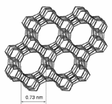
Figure 15: Structure of the hexagonal AlPO₄-5 molecular sieve. The corners of the polygons are occupied alternately with aluminum and phosphorus, while the polygon sides represent oxygen. The hexagonal $c$-axis is oriented along the channel pores.

Pure AlPO₄-5 crystals are optically transparent from below 400 nm to above 800 nm and exhibit a refractive index of $n(500\,{\rm nm})=1.466$. After removing the template (usually by heating) they show practically no birefringent properties. X-ray diffraction revealed patterns which are consistent with space group $\rm P\frac{6}{\rm m}cc$ as well as P6cc. The latter group, however, corresponds to a polar structure: In fact, the 4 in the formula AlPO₄-5 is the result of the strict alternation of Al and P in the tetrahedral nodes of the framework, which prevents the corner-sharing oxygen tetrahedra to occur with odd numbers, and which leads to an alternating stacking of Al and P in the direction of the channels ($c$-axis); cf. Fig. 15. This alternance is assumed to cause the crystallographic polar nature [95] of the framework [96]. The macroscopic polar nature of AlPO₄-5 single crystals was proven recently in scanning pyroelectric microscopy investigations [97], and it was observed that AlPO₄-5 crystals are usually twinned. The murky stripes inside the pyridine 2-loaded crystals shown in Fig. 18 and their slightly bowed side faces could well be a result of this kind of twinning. At this moment it is not clear, however, to what extent twinning should affect the properties relevant for luminescence and lasing discussed here.

Up to now laser action was obtained in two different compounds, namely in AlPO₄-5 loaded with 1-ethyl-4-(4-(p-dimethylaminophenyl)-1,3-butadienyl)-pyridinium perchlorate (pyridine 2 [98]), and with a modified rhodamine B dye. In the following we will discuss the two materials in more detail.

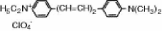
Figure 16: Structure formula of the dye 1-ethyl-4-(4-(p-dimethylaminophenyl)-1,3-butadienyl)-pyridinium perchlorate (pyridine 2 [98]); molecular mass 378.9 g/mol.

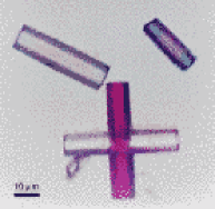
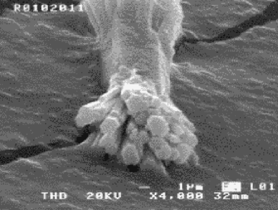
Figure 17: Morphology of typical pyridine 2/AlPO₄-5 crystals; left: without lasing properties, right: with lasing properties.

7.1.1 AlPO4-5/pyridine2 compound

These AlPO₄-5–dye compounds were synthesized [99] following a procedure in which the dye 1-ethyl-4-(4-(p-dimethylaminophenyl)-1,3-butadienyl)-pyridinium perchlorate (trade name pyridine 2 [98]), cf. Fig. 16, is added to the template or to the aluminum hydroxide suspension [100, 101, 102]. After 1 h of hydrothermal synthesis dark red crystals with a length of up to 100 $\mu$m are obtained. As the linear dye molecules fit snugly into the 0.73 nm wide channel pores of the nanoporous AlPO₄-5 host, they become aligned along the crystal $c$-axis. As a result the compound exhibits strong dichroism, and the emitted fluorescence light is polarized parallel to the $c$-axis. This is documented in Fig. 18. It is also observed that with the inclusion of pyridine 2 the entire compound acquires pyroelectric properties and an optical second order susceptibility [3].

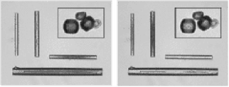
Figure 18: Transmission micrographs of the dichroism in dye-loaded AlPO₄-5 crystals; the rod-shaped crystals contain ca. 0.1 wt-% or 1 pyridine 2 molecule per 260 unit cells, while the barrel-shaped ones (shown in the inset) enclose rhodamine BE50 (ca. 0.5 wt-% or 1 molecule per 75 unit cells). Only the polarization component parallel to the optical transition moment of the molecules is absorbed. In the rod-shaped crystal the pyridine 2 dyes are completely aligned, whereas with the rhodamine BE50 dye in the barrel-shaped crystals we observe only a weak dependence of the color upon the incident polarization. Left: incident light horizontally polarized; Right: incident light vertically polarized.

Even though the size of the dye molecules is well compatible with the channel diameter, the dye content visibly affects the crystal morphology. Regular hexagonal crystals with a rodlike form, as e.g. the ones shown in Fig. 17(left), or Fig. 18, are obtained when the dye content is low, around 0.1 wt% or 1 molecule per 260 unit cells. At higher concentrations the dye accumulates in the middle of the crystal, and the disturbances grow: at a dye content of $\gtrapprox$ 0.2 wt%, crystals with a characteristic fascicular shape resulted; cf. Fig 17(right). Given the small size of the crystals the dye content was determined by chemically dissolving them. With this method, however, it is not possible to accurately determine the spatial distribution of the dye. Therefore the content was also evaluated qualitatively by comparing the depth of the color. It is only with these fascicled pyridine 2-loaded crystals where laser emission was observed. Apparently, in the undisturbed rod-shaped crystals the low concentration of dye does not spoil the growth, but it is not sufficient to provide the necessary optical gain for compensating all losses either.

7.1.2 AlPO4-5/rhodamine BE50 compound

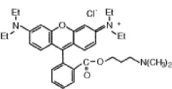
Figure 19: Structure formula of the new dye rhodamine BE50 (ethanaminium, $N$-[6-(diethylamino)-9-[2-($N,N$-dimethyl-3-amino-1-propoxycarbonyl)phenyl]-3H-xanthen-3-ylidene]-$N$-ethyl-chloride) molecular mass 564 g/mol [103].

The second molecular sieve dye compound which exhibited lasing properties was obtained by including a modified rhodamine B dye in an AlPO₄-5 crystal. The size of rhodamine molecules exceeds the dimensions of the channel pores in AlPO₄-5 crystals. As a result the rhodamine B is normally not accepted inside crystal pores but adheres at the exterior. The group of Schulz-Ekloff and Wöhrle started an attempt to accomplish rhodamine inclusion in AlPO₄-5 crystals, even so the pores are too small. Their idea is to modify the dye molecule in a way that makes the dye molecule electrically resemble a template molecule. Their new derivative rhodamine BE50 (ethanaminium, $N$-[6-(diethylamino)-9-[2-($N,N$-dimethyl-3-amino-1-propoxycarbonyl)phenyl]-3H-xanthen-3-ylidene]-$N$-ethyl-chloride; cf. Fig. 19) was synthesized by esterification of rhodamine B (Rh B) with 3-dimethylamino-1-propanol [103]. It was shown that the concentration of rhodamine BE50 (Rh BE50) achievable by crystallization inclusion in AlPO₄-5 exceeds the possible Rh B concentration by a factor of 3–4. This was attributed to the different molecule structures, i.e., to the zwitterionic nature of Rh B on one hand, and to the additional positive charge of a protonated aliphatic amino group of Rh BE50 on the other hand [103]. The latter molecules with the localized positive charge are more compatible with the AlPO₄-5 framework than the delocalized charge of Rh B. As a consequence they observe that at a given dye concentration Rh BE50 inclusion leads to a better crystal morphology than Rh B inclusion [104].

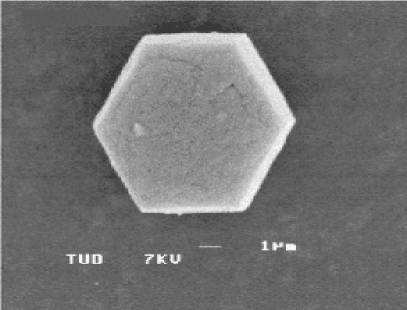
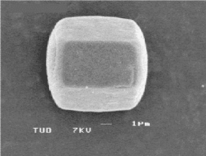
Figure 20: Morphology of typical rhodamine BE50/AlPO₄-5 crystals with lasing properties; dye content ca. 0.5 wt-% or 1 dye molecule per 75 unit cells.

The gel for the synthesis of the AlPO₄ crystals is prepared according to recipes [95, 105] which are modified for the purpose of crystallization inclusion of dyes [106]. To a suspension of 61.6 mmol $\rm Al_{2}O_{3}$ as aluminum source [107] and 75 g deionized water, 61.6 mmol $\rm P_{2}O_{5}$ [108] in 11.3 g deionized water is added under mechanical stirring. After 5 min a uniform gel formed and then 92.4 mmol tripropylamine [109] is added slowly. Subsequently, the appropriate amount (0.1–10 mmol) of Rh BE50 dye powder is mixed with the gel. The synthesis of the Rh BE50/AlPO₄-5 crystals is performed by microwave heating [110], which proved to be superior in respect of avoiding damage of sensitive dyes like coumarines [111] as well as of reducing the time of synthesis [103]. Unlike the pyridine 2 molecules, which with a diameter of 0.6 nm fit into the 0.73 nm wide pores of the AlPO₄-5 host, the Rh BE50 molecules with dimension of 0.91 $\times$ 1.36 nm² are accommodated in defect sites, or mesopores, of the host crystal. Remarkably, up to concentrations of 1 molecule per 75 unit cells this remains without any visible negative consequences for the crystal morphology, as is documented in Fig. 20.

In Fig. 18 the dichroic properties of the compound are illustrated. In comparison with the pyridine-2/AlPO₄-5 compound, the dichroism of the Rh BE50 compound is reduced and the fluorescence emission is only partially polarized. This is an indication that the electrical anisotropy of the host structure does not fully carry through the mesopores, resulting in a weak dye alignment in the statistical average.

7.2 Microresonator structure

As is visible in Fig. 18 – and as the polarization of the emitted fluorescence of the compounds indicates – the absorption, as well as the emission dipole moment of the included dyes are oriented preferentially along the crystal $c$-axis (in the pyridine 2/AlPO₄-5 compound the orientation is complete). As dipole emission along the dipole axis is not possible, the emission parallel to a plane perpendicular to the prevailing dipole orientation (i.e. the hexagonal axis) is enhanced. Here a bundle of emission directions meets the condition for total internal reflection (TIR) at the hexagonal side faces inside the crystal. In a whispering-gallery-mode-like way the corresponding emission can circulate sufficiently often to accumulate the gain required to overcome the lasing threshold; cf. Fig. 2 in which this intuitive model is illustrated for a particular ray bundle of high symmetry. However in section 6 we have shown that for resonators with a sizes in the order of a few wavelengths the naive ray picture does not correctly represent the field modes. E.g. the ray picture insinuates a mode concentration in the center of the faces but field-free corners. This, however, is not consistent with the experimental evidence, which clearly shows that the emission occurs at the corners; cf. Fig. 26. As we already pointed out in section 6.13, the main feature that distinguishes the hexagonal resonator from other common whispering-gallery type cavities such as microdroplets [112] or semiconductor disk lasers [67, 113], is that the latter do not exhibit sharp corners and flat sides. There we described that portions of the boundary in convex resonators act as focussing or defocussing elements, whereas the straight sides of a hexagon are neither one nor the other. As a result we have shown that ray paths in the hexagon display a degree of complexity that cannot be classified as chaotic and was called pseudointegrable.

The closed ray path underlying Fig. 2 is only one member of an infinite family of periodic orbits of the hexagon billiard that all have the same length, $L=3\times WoF$. Long-lived cavity modes exist only if the corresponding rays satisfy the condition of TIR at the interface, $\sin\chi>1/n$, where $\chi$ is the angle of incidence with respect to the surface normal. In a naive ray approach one would furthermore obtain the spectrum of modes by requiring an integer number of half wavelengths to fit into $L$, leading to constructive interference on a round-trip. As we shall see shortly, this estimate is justified, even though a proper treatment of the ray-wave connection has to take into account that any given mode is in fact made up of a whole family of different ray paths. The ultimate breakdown of the ray model, however, occurs when a ray orbit hits the corners where the classical laws of refraction and reflection are no longer defined. To characterize the size of the samples, we can specify either the radius $R$ of the hexagon at the corner points or – more conveniently – the width over flats (WoF) characterized by $R=WoF/\sqrt{3}$.

7.2.1 Wave picture: spectral properties

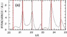
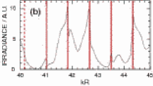
Figure 21: Calculated scattering intensity spectra of a hexagonal cylinder for plane-wave incidence at $15^{\circ}$ to a side face and detection at $60^{\circ}$ from incidence. (a) corresponds to a spectral interval $\lambda\approx 653\ldots 816$ nm for width over flats (WoF) $4.5\,\mu$m; (b) covers the interval $\lambda\approx 605\ldots 680$ nm for WoF $7.5\,\mu$m. Vertical lines are guides to the eye, indicating narrow resonances. The spacing between resonances is $\Delta(kR)\approx 0.84$ in (a) and $\Delta(kR)\approx 0.83$ in (b), in good agreement with the characteristic mode spacing $\Delta(kR)_{c}\approx 0.83$ of a closed hexagonal orbit. Expected resonances not clearly seen in the above spectra are marked by dashed lines; they appear at other detection angles.

Because the hexagonal faces are neither focussing nor defocussing, there is no obvious way of determining the weight that should be given to individual members of a ray family in order to predict the spatial structure of the resulting mode. Full solutions of Maxwell’s equations have therefore been carried out for the TM polarized modes of a dielectric hexagonal prism, using methods previously applied in [67, 113] and discussed in section 6. In anticipation of the experimental spectra discussed in section 7.3, we focus on three different sample sizes characterized by a WoF of $4.5\,\mu$m, $7.5\,\mu$m, and $22\,\mu$m. The aim is to understand the observed laser line spacings and the emission directionality.

To document that orbits of different families determine the characteristic mode spacing of the cavity, Fig. 21 shows scattering spectra for different sample sizes in the vicinity of the experimental wavelengths. Intensity is plotted versus dimensionless wavenumber $kR$, where $k=2\pi/\lambda$. This is the natural scale for comparison with semiclassical predictions because modes differing by one node along a closed path should then be equally spaced, with a characteristic separation $\Delta(kR)_{c}=2\pi\,R/(n\,L)=2\pi/(3\sqrt{3}n)=0.825$ independent of the sample size. The expected wavelength spacing of the modes (free spectral range $FSR$) is $\Delta\lambda=\lambda^{2}\times\Delta(kR)_{c}/(2\pi R)\approx 23$ nm in (a) and $\Delta\lambda\approx 11$ nm in (b). For $WoF=22\,\mu$m, we obtain $\Delta\lambda\approx 4.9$ nm. Figure 21 indeed shows a series of resonant features with approximately the predicted wavevector spacing.

Each of the peaks marked in Fig. 21(b) is in fact a multiplet which is not resolved, because the splittings of the individual modes comprising the multiplet are smaller than their passive linewidths. There is evidence for this because several of the peaks are very asymmetric, and in particular exhibit a steep slope on one side. For an isolated resonance, the most general lineshape that could arise is the Fano function (of which the Lorentzian is a special case), which however does not yield satisfactory fits here.

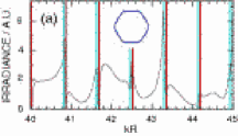
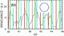
Figure 22: Calculated scattering intensity spectra for slightly rounded hexagonal cavities (shapes depicted as insets). The incoming plane wave is at an angle of $15^{\circ}$ to a facet in (a) and $30^{\circ}$ in (b); detection occurs at $60^{\circ}$ from incidence. Spacings between modes of the same color agree well with $\Delta(kR)_{c}\approx 0.83$, cf. Fig. 21. All resonances in (a) appear as doublets. At $kR\approx 42.5$ the doublet structure is seen most clearly. In (b), stronger deviation from hexagonal shape leads to further lifting of degeneracies. Dashed lines mark expected resonances not seen at this observation angle.

To further expose the multiplet structure, we modeled deviations from the ideal hexagonal shape which could lead to narrower individual linewidths and increase the multiplet splitting. Shape perturbations were chosen that preserve the $D_{6h}$ point group symmetry and hence remove only “accidental” quasi-degeneracies. The actual perturbation that is present in the samples of Figs. 24 and 25 eluded experimental characterization, so that a model calculation can reproduce only generic features which are insensitive to the precise type of perturbation. One such feature is the average mode spacing after degeneracies have been lifted sufficiently.

Figure 22(a) shows the spectrum of a rounded hexagon where the radius of curvature at the corners is $\rho\approx 0.9\,\lambda$ (assuming $\lambda\approx 610$ nm for definiteness). No qualitative difference to Fig. 21(b) is seen, except that the resonant features have become somewhat narrower, thus enabling us to identify two distinct series of modes with caracteristic spacing $\Delta(kR)_{c}$. This indicates that departures from sharp corners are not resolved in the wave equation when their scale is smaller than $\lambda$. A qualitatively different spectrum is observed in Fig. 22(b) where $\rho\approx 3.7\,\lambda$. Here, the perturbation reveals three well-separated, interpenetrating combs of modes, again with period $\Delta(kR)_{c}$. There are $21$ distinct resonances in the wavelength interval of Fig. 22(b), which translates to an average mode spacing of $\Delta\lambda\approx 3.6$ nm for a $WoF=7.5\;\mu$m resonator, well in agreement with the experiment; cf. Fig. 25.

In order to verify that no further modes will be revealed by other choices of deformation, an independent estimate of the average density of modes can be made based on semiclassical considerations [114]:

$$\left\langle\frac{dN}{d(kR)}\right\rangle = \frac{n^{2}\,k\,R}{4}$$ (367)

$$\times \left[1-\frac{2}{\pi}\,\left(\arcsin{\frac{1}{n}}+\frac{1}{n}\,\sqrt{1-\frac{1}{n^{2}}}\right)\right]$$

Here, $dN$ is the number of modes in the interval $d(kR)$. The result is $\langle\frac{dN}{d(kR)}\rangle\approx 4.6$, and hence we expect $\approx 22$ modes in the interval of Fig. 22(b), again in good agreement with the actual count.

7.2.2 Wave picture: intensity profile

There is one class of quasi-degeneracies that is not removed by any of the perturbations in Fig. 22. Their physical origin is time reversal symmetry for the ray motion inside the cavity. Any of the periodic orbits can be traversed either clockwise or counterclockwise, and the same holds for more general ray paths. The different propagation directions can be linearly combined in various ways to obtain nearly-degenerate standing-wave patterns that differ only in their parity with respect to some of the crystal’s reflection axes. A minute splitting does exist because the nonintegrability of the ray motion implies that the propagation direction itself is not a “good quantum number”, i.e. reversals of the sense of rotation are unlikely but not impossible in the wave equation. This is analogous to quantum tunneling and hence leads only to exponentially small splittings that can be neglected on the scale of the individual resonance linewidths [115]. These multiplets have been counted as one resonance in (367).

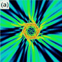
Figure 23: False-color representation of the cross-sectional intensity in the ideal hexagon for a mode with (a) $kR=22.89$ [cf. Fig. 21 (a)] and (b) $kR=42.78$ [cf. Fig. 21 (b)]. The resonance width is $\delta(kR)=0.10$ in (a) and $\delta(kR)=0.04$ in (b).

Following this reasoning, in Fig. 23 the traveling-wave patterns belonging to one of the resonances in Fig. 21(a) and (b), respectively, is plotted. High intensity ridges inside the resonator form a whispering-gallery-like pattern that decays from the interface into the cavity center. The number of ridges in the radial direction (perpendicular to a side face) provides an approximate analogue of a transverse mode order, however upon closer examination one sees that the number of ridges and nodal lines is not uniquely defined, in particular along a diameter joining opposite corners. The modes can therefore not be properly labeled by “good quantum numbers” characterizing the number of radial and azimuthal nodes – this is a direct consequence of the nonintegrability of the problem. The most significant difference to the whispering-gallery modes of a circular cavity is clearly the anisotropic emission. High intensity is seen to emanate predominantly from the corners and is directed almost parallel to an adjacent crystal facet. The overall emission pattern is very similar in both modes despite the large difference in size (or $kR$) between the two hexagons.

7.3 Laser properties

The dye loaded molecular sieve microcrystals presented in section 7.1.1 and 7.1.2 were excited with 10 ns pulses from the 532 nm second harmonic of a Nd:YAG-laser, and the emitted luminescence was collected with a 42^∘ aperture lens relaying the microlaser emission to a spectrometer and an imaging system consisting of a cooled low noise CCD-camera.

7.3.1 Pyridine2 AlPO4-5 compound

In Fig. 24 the emission and lasing spectra of three pyridine 2-loaded compounds with different dye content are compared. Fig. 24a represents the class of regularly shaped samples with a low dye content around 0.1 wt% [cf. also Fig. 17(left)]. In this class the fluorescence emission maximum was observed between 645 nm to 665 nm, where the shift to longer wavelength correlates with the increase of dye content that was assessed by the saturation of the red color. In none of these rod-shaped crystals laser emission was observed.

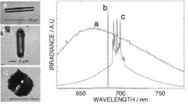
Figure 24: Emission and lasing spectra of different pyridine 2-loaded compounds with from a to c increasing amounts of included dye. The dye concentration was estimated empirically based on the sample color depth. The width over flats of sample b is 4 $\mu$m. The free spectral range (FSR) of this resonator is so large (ca. 25 nm) that only one emission mode acquires the available gain, resulting in single line emission. On the other hand, sample c is ca. 5 times larger. In this case the FSR is around 5 nm so that laser emission can occur on a multitude of modes simultaneously.

However, narrow laser emission peaks were observed in fascicled samples with a detected linewidth of ca. 0.3 nm which was limited by the spectrometer resolution. Here the emission maxima were observed at wavelenghts up to 695 nm, and again, increasing dye concentration correlated with increasing redshift (cf. Figs. 24b and c). As already mentioned, together with the increasing dye content the crystal morphology becomes more and more disturbed. The observation of a disturbed morphology and the red-shift of the emission spectrum are consistent with the hypothesis of a host-guest interaction which increases with dye content. In fact both, the pyridine 2 molecules, as well as the AlPO₄-5 framework, carry a static dipole moment [95, 96]. As a consequence, the increased buildup of electrostatic energy in the crystal lattice has to be compensated by an increasing amount of stacking faults. On the other side, the mechanism of the redshift is not unequivocally identified, yet, but is probably related to the one discussed in [116, 117].

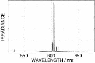
Figure 25: Lasing spectrum of a rhodamine BE50-loaded AlPO₄-5 microcrystal with a concentration around 75 unit cells per dye molecule and size of 7.5 $\mu$m width over flats.

7.3.2 Rhodamine BE50 AlPO4-5 compound

Also with these samples the same correlation between the emission wavelength and dye concentration was observed; cf. also [103]. In contrast to the pyridine 2-loaded samples, the fluorescence emission was not completely polarized. The observed polarization contrast $c_{p}=\frac{I_{\parallel}-I_{\perp}}{I_{\parallel}+I_{\perp}}$ was around 10%, indicating that in the average the Rh BE50 molecules are only weakly aligned with respect to the host crystal. Laser emission was observed in samples with a dye concentration around 75 unit cells per dye molecule, corresponding to 0.5 wt%; cf. Fig. 25.

7.3.3 Laser properties of molecular sieve dye compounds

Independent of the type of loading, in most microcrystals with $WoF\gtrapprox$ 8 $\mu$m lasing was observed to occur on several sharp lines with instrument resolution limited width (a typical example is shown in Fig. 25). In general the laser emission lines are not equally spaced. In fact, the free spectral range ($FSR$) of 11 nm corresponding to the resonator size of $WoF=8\;\mu$m is far above the line spacing of 3.2, 4.3 and 3.4 nm shown in Fig. 25. This is in agreement with the theoretical model of paragraph 7.2.1, in which the average lasing mode spacing (after lifting the quasi-degeneracies in the ideal hexagon) was estimated to be $\Delta\lambda=$ 3.6 nm. Also in agreement with the theoretical discussion are the regions where the laser light leaves the hexagonal resonators. Figure 26(left) shows the laser emission as bright spots. Clearly the emission is concentrated along the crystal edges. The complex emission distribution is compatible with the simultaneously recorded spectrum (cf. Fig. 25) which reveals emission on four modes.

While the average line spacing of 3.6 nm observed in the sample of Fig. 25 is not compatible with the free spectral range of $\Delta\lambda=12$ nm of the corresponding resonator, the 4.2 nm spacing of the 3 dominant peaks in the sample shown in Fig. 24c is in accord with the $FSR$ resulting from the 22-$\mu$m-WoF hexagonal resonator. On the other hand, the theoretical model for the $22\,\mu$m-WoF hexagonal resonator (cf. Eq. (367)) yields an average mode spacing of $\Delta\lambda\approx$ 0.5 nm which is close to the spectrometer resolution. This high spectral density explains the large background in the lasing spectrum of Fig. 24: It is likely that not all the individual lasing modes in this sample are resolved, and hence part of the shoulder on which the three peaks of curve c sit is probably shaped by a series of closely spaced lasing modes.

On the other hand, samples with smaller resonator ($WoF\gtrapprox$ 4 $\mu$m), as e.g. the one shown in Fig. 24b, emitted one single laser line. Thus the emission is unadulterated by hole burning induced multimode beating and interference, and this results in the simple emission pattern shown in Fig 26(right), where two ca. 1 $\mu$m-spots ($\approx$ microscope resolution limit) mark the region of laser emission, which, again, is located at the crystal edges. Remarkably, compared to larger samples, the ratio of the line peak to the underlying fluorescence shoulder of these small lasers is an order of magnitude higher (cf. Figs. 24 and 27).

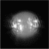
Figure 26: Patterns of the laser emission show that the emission originates from regions along side edges. Left: rhodamine BE50/AlPO₄-5 compound; width over flats 7.5 $\mu$m. An electron micrograph of the sample is shown in Fig. 20 with horizontal $c$-axis. Here the $c$-axis orientation is nearly vertical. The corresponding emission spectrum is shown in Fig. 25. Right: pyridine 2/AlPO₄-5 compound; width over flats 4.5 $\mu$m. The corresponding sample and emission spectrum is represented in Fig. 24 b.

7.3.4 Laser threshold

Figure 27 illustrates the differential efficiency behavior of a typical microlaser with $WoF<10\,\mu$m and one with $WoF>10\,\mu$m. Lasing threshold for the latter size samples was around 0.5 MW/cm², regardless of the type of dye loading. On the other side, crystals of smaller size ($WoF=4\;\mu$m) from the same synthesis batch revealed a considerably smaller threshold (0.12 MW/cm²) and a factor of $>7$ larger differential gain. We assume that this is a consequence of the quantum size effects which we described in section 5.

It is informative to compare the threshold of molecular sieve microlasers with vertical cavity surface emitting lasers (VCSELs). For that we convert the pump irradiance $I$ (incident optical power per unit area) into a flux of photons $\phi$ (number of pump photons per second incident on the mode cross section $A$)

$$\phi=\frac{I\;A}{h\,\nu}=\frac{I\;A\;\lambda_{p}}{h\,c}\;.$$ (368)

If $\eta$ denotes the efficiency with which an incident pump photon actually contributes to an excitation, then $\phi\times\eta$ corresponds to the number of quantum processes per second required to reach a given level of inversion. Multiplication of this number with the charge of an electron $q_{e}=1.6\times 10^{-19}$As gives the electric current which corresponds to the pump current flowing in a comparable electric device, such as a VCSEL. According to (368) the threshold power density of 0.12 MW/cm² incident on the surface of the molecular sieve laser shown in Fig. 24b of $1\times 4\;\mu$m (cf. Fig. 26b) corresponds to a flux of $1.4\times 10^{16}$ s^-1 532-nm-photons. If we take into account that the pump field was not polarized, but the dye molecules are aligned, then only 50% of the pump photons could contribute to the inversion. In addition the absorption length for 532 nm radiation is longer than the crystal size so that only a fraction of the incident pump is absorbed by the dye molecules. If we assume that 50% of the pump are absorbed, then the effects of polarization and absorbtion length together result in a quantum efficiency of $\eta=0.25$. With this quantum efficiency we obtain a comparable electric threshold current of 560 $\mu$A, which compares well with the threshold current of VCSELs of comparable size. Thus, in terms of elementary (quantum) pump processes needed to reach lasing threshold the molecular sieve lasers are as good as actual VCSELs.

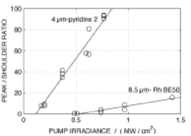
Figure 27: Lasing threshold and differential efficiency of typical AlPO₄-5/dye compounds. Shown is the peak of the laser emission spectrum normalized by the fluorescence shoulder as a function of the pump power density for the sample shown in Figs. 24b and 25.

7.4 Photostability

Photostability is usually a critical issue with organic dyes. Corresponding investigations were carried out with pyridine 2, as well as rhodamine BE50 loaded samples, revealing some unexpected results.

7.4.1 Photostability of pyridine 2 compounds

The photostability of pyridine 2 compounds was studied with samples exhibiting an undisturbed morphology, similar to the one shown in Fig. 18. The samples were irradiated with 10 Hz trains of 10 ns pulses of the 532 nm second harmonic of a Nd:YAG-laser and a power density of 5 MW/cm². Figure 28 illustrates the wane of fluorescence activity of a pyridine 2-loaded AlPO₄-5 sample under such bleaching irradiation. After a bleaching period of 140 seconds the exposure was interrupted for 18 minutes. Then the bleaching procedure was resumed. The figure shows that the fluorescence recovers during the intermission.

The physical origin of this unexpected fluorescence recovery is not clear yet. If we assume that bleaching consists in breaking bonds of the dye molecules, then we have to consider bond energies in the eV-range. Even if we assume that the dye debris stay encaged in their pores, spontaneous or thermally activated self healing of broken eV-bonds seems not very probable. Considering the stereometrically restricted possibilities inside the molecular sieve framework together with diffusion distances of several $\mu$m, and the observed recovery time in the range of minutes, we believe that diffusion of new, intact dye molecules into the irradiated crystal volume is more plausible than self healing.

Figure 28: Fluorescence activity of a pyridine 2-loaded AlPO₄-5 sample under bleaching laser irradiation. Left: Micrograph of the sample crystal. Center: Fluorescence activity as a function of time: After a first bleach period of 140 seconds the bleach beam is interrupted for 18 minutes. During this intermission the fluorescence recovers to start the second bleach period with $3\times$ stronger emission. Right: The bleaching laser is incident from the left and concentrated in the center of the crystal. Shown is the fluorescence distribution at the end of the first bleach period of 140 s. Clearly visible is the bleached hole in the center, where the bleach beam was concentrated.

As bleaching reduces the concentration of dye, a blueshift of the fluorescence is expected with increasing photobleaching [95, 96]. However, the 656-nm-fluorescence emission maximum of this sample is already at the shortest observed wavelength (cf. Fig. 24), corresponding to a low dye concentration, and consequently, to weak dipole interactions. Thus, the blueshift under these circumstances must be rather small. This explains that a blueshift was not observed with these pyridine 2-loaded samples.

7.4.2 Photostability of rhodamine BE50 compounds

The rhodamine BE50-loaded samples under investigation contained dye at a concentration of around one Rh BE50 molecule per 75 unit cells, and therefore bleaching caused a detectable 4 nm shift of the fluorescence towards the blue. The 532 nm bleach irradiance was 0.5 MW/cm² with this samples. In contrast to the pyridine 2 samples these crystals exhibited laser emission. Observing the laser emission spectrum while bleaching the samples, a further consequence of the blueshift was revealed: Blueshift of the fluorescence reduces the overlap of the fluorescence band with the absorption spectrum, and as a result, laser modes at lower wavelengths will suffer less losses with increasing bleaching. This is documented in Fig. 29, where the intensity of mode b with the shortest oscillating wavelength increases, while longer-wavelength-modes a and c decrease during the bleach procedure. At the same time a 0.2 nm blueshift of the oscillation wavelength was detected. We attribute this to a weak decrease of the refractive index of the resonator material due to the smaller polarizability of the dye debris. In contrast to the pyridine 2 samples, however, recovery of the fluorescence was not detected. As we mentioned in section 7.1.2 the Rh 50BE molecules are considerably larger than pyridine 2 molecules, and are encaged in mesopores. As a result their mobility in the molecular sieve framework is severly hampered. So, diffusion of intact molecules into the bleached volume occurs – if ever – on timescales considerably larger than minutes. This is probably the reason why fluorescence recovery was not observed in rhodamine BE50 compounds.

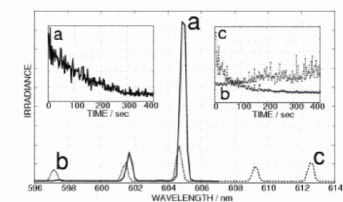
Figure 29: Effect of photobleaching on the laser emission intensity: short wavelength line b grows with progressive bleaching, while longer wavelength lines a and c decrease.

8 Conclusion

This chapter was centered on microscopic lasers realized with nanoporous materials, especially molecular sieve dye compounds. We discussed the effects of a microresonator on spontaneous and stimulated emission properties, and we showed that wavelength scale laser resonators may exhibit lasing without threshold. Such effects are not just thoughtful observations, but were investigated in real devices as well, and we reviewed observations of threshold reduction in molecular sieve lasers.

The microresonators of the molecular sieve lasers which were presented up to now exhibit a hexagonal resonator geometry. Hexagonal microresonators in which the light field is confined by total internal reflection at the dielectric boundary define a new class of pseudointegrable optical structure of which we reviewed the properties in some detail.

As mentioned, molecular sieve microlasers can be fabricated in large amounts with the same large scale processes which are used to produce the molecular sieve crystallites in the petrochemical industry. Although applications of such laser powders have not been reported yet, many practical uses can be envisaged, such as for example in efficient fluorescent, or even lasing paint pigments or lasing pixels.

8.1 Acknowledgements

We thank the following individuals for their help in preparing this text as well as for their contributions on the way to realize lasing in molecular sieves: P. Behrens, I. Braun, G. Ihlein, O. Krauß, F. Marlow, G. Schulz-Ekloff, F. Schüth, U. Vietze, Ö. Weiss, and D. Wöhrle. Some of the work reviewed here was supported by the “Deutsche Forschungsgemeinschaft” and the “Max-Planck-Gesellschaft”.

References

- [1] J. Kräger, K. Hahn, V. Kukla, and C. Rödenbeck, Phys. Bl., 54, 811 (1998)
- [2] N. Gfeller, S. Megelski, and G. Calzaferri, J. Phys. Chem. B 102, (1998) 2433; J. Phys. Chem. B 103, 1250 (1999)
- [3] U. Vietze, O. Krauß, F. Laeri, G. Ihlein, F. Schüth, B. Limburg, and M. Abraham, Phys. Rev. Lett., 81, 4628 (1998)
- [4] R. P. Feynman, R. B. Leighton, and M. Sands, The Feynman Lectures on Physics Vol. II, Addison-Wesley, Reading (Massachusetts), 1964, p. II-27-5
- [5] E. Merzbacher, Quantum Mechanics, 2nd. edn., Wiley, New York, 1970, S. 356
- [6] W. Heitler, The Quantum Theory of Radiation, 3rd. edn., Oxford University Press, London, 1954
- [7] W. H. Louisell, Quantum Statistical Properties of Radiation, Wiley, New York, 1973
- [8] R. J. Glauber, Phys. Rev., 131, 2766 (1963)
- [9] T. Basché, W. E. Moerner, M. Orrit, and U. P. Wild, eds., Single-Molecule Optical Detection, Imaging, and Spectroscopy, VCH-Verlagsgesellschaft, Weinheim (Germany), 1996
- [10] W. E. Moerner and M. Orrit, Science 283, 1670 (1999).
- [11] L. Allen and J. H. Eberley, Optical resonance and two-level atoms and ions, Wiley, New York, 1975
- [12] I. I. Rabi, Phys. Rev., 51, 652 (1937)
- [13] F. Bloch, Phys. Rev., 70, 460 (1946)
- [14] L. I. Schiff, Quantum mechnics, McGraw-Hill, New York, 1968
- [15] E. Hecht, Optics; 2nd ed., Addison-Wesley, Reading, 1987, p. 322.
- [16] R. P. Feynman, F. L. Vernon, and R. W. Hellwarth, J. Appl. Phys., 28, 49 (1957)
- [17] H. Walther, Phys. Bl., 33, 653 (1977)
- [18] M. Dagenais and L. Mandel, Phys. Rev. A, 18, 2217 (1978)
- [19] B. W. Shore, P. Meystre, and S. Stenholm, J. Opt. Soc. B., 8, 903 (1991)
- [20] V. Weisskopf and E. P. Wigner, Z. Phys., 63, 54 (1930)
- [21] P. Meystre ans M. Sargent III, Elements of Quantum Optics, 2nd ed., Springer, Berlin, 1991
- [22] N. Gisin and I. Percival, Phys. Rev. A, 46, 4382 (1992)
- [23] K. Moelmer, Y. Castin, and J. Dalibard, J. Opt. Soc. Am. B, 10, 524 (1993)
- [24] E. M. Purcell, Phys. Rev., 69, 681 (1946)
- [25] D. Kleppner, Phys. Rev. Lett., 47, 233 (1981)
- [26] M. G. Raizen, R. J. Thompson, R. J. Brecha, H. J. Kimble, and H. J. Carmichael, Phys. Rev. Lett., 63, 240 (1989)
- [27] F. Bernardot, P. Nussenzweig, M. Brune, J. M. Raimond, and S. Haroche, Europhys. Lett., 17, 33 (1992)
- [28] A. E. Siegman, Lasers, University Science Books, Mill Valley(CA), 1986
- [29] J. Parker and C. R. Stroud, Phys. Rev. A, 35, 4226 (1987)
- [30] R. G. Cook and P. W. Milonni, Phys. Rev. A, 35, 5071 (1987)
- [31] H. J. Carmichael, R. J. Brecha, M. G. Raizen, H. J. Kimble, and P. R. Rice, Phys. Rev. A, 40, 5516 (1989)
- [32] E. T. Jaynes and F. W. Cummings, Proc. IEEE, 51, 89 (1963)
- [33] D. Meschede, H. Walter, and G. Müller, Phys. Rev. Lett., 54, 551 (1985)
- [34] H. Yokoyama, K. Nishi, T. Anan, Y. Nambu, S. D. Brorson, E. P. Ippen, and M. Suzuki, Opt. Quantum Electron., 24, S245 (1992)
- [35] F. De Martini and G. R. Jacobovitz, Phys. Rev. Lett., 60, 1711 (1988)
- [36] K. J. Blow, R. Loudon, S. J. D. Phoenix, and T. J. Shepherd, Phys. Rev. A, 42, 4102 (1990)
- [37] J. D. Jackson, Classical electrodynamics, 3rd ed., Wiley, New York, 1998
- [38] R. J. Glauber and M. Lewenstein, Phys. Rev. A, 43, 467 (1991)
- [39] S. Scheel, L. Knöll, and D. G. Welsch, Phys. Rev. A, 58, 700 (1998)
- [40] R. Houdré, C. Weisbuch, R. P. Stanley, U. Oesterle, P. Pellandini, and M. Ilegems, Phys. Rev. Lett., 73, 2043 (1994)
- [41] V. V. Klimov, M. Ducloy, and V. S. Letokhov, Phys. Rev. A, 59, 2996 (1999)
- [42] T. B. A. Senior and J. L. Volakis, Approximate boundary conditions in electromagnetics, IEE Electromagnetic waves series 41, London, 1995
- [43] L. G. Guimares, H. M. Nussenzveig, and W. J. Wiscombe, Opt. Commun., 89, 363 (1992)
- [44] M. C. Cross and P. C. Hohenberg, Rev. Mod. Phys., 65, 851 (1993)
- [45] C. O. Weiss, M. Vaupel, K. Staliunas, G. Slekys, V. B. Taranenko, Appl. Phys. B, 68, 151 (1999); C. O. Weiss, Phys. Rep., 219, 311 (1992)
- [46] H. C. van de Hulst, Light scattering by small particles, Dover Publications, New York, 1981
- [47] M. Kerker, The scattering of light and other Electromagnetic Radiation, Academic Press, New York, 1969
- [48] P. W. Barber and S. C. Hill, Light scattering by particles: Computational methods, World Scientific, Singapore (1990)
- [49] A. W. Snyder and J. D. Love, Optical waveguide theory, Chapman and Hall, London (1991)
- [50] A. W. Poon, R. K. Chang, and J. A. Lock, Opt. Lett., 23, 1105 (1998)
- [51] J. C. Ahn, K. S. Kwak, B. H. Park, H. Y. Kang, J. Y. Kim, and O’Dae Kwon, Phys. Rev. Lett., 82, 536 (1999)
- [52] R. Courant and D. Hilbert, Methoden der Mathematischen Physik I, Springer, Berlin, 1968
- [53] B. R. Johnson, J. Opt. Soc. Am. A, 10, 343 (1993)
- [54] J. U. Nöckel and A. D. Stone, in: Optical processes in microcavities, edited by R. K. Chang and A. J. Campillo, World Scientific, Singapore, 1996
- [55] J. U. Nöckel, PhD Thesis, Yale University (1997)
- [56] U. Fano, Phys. Rev., 124, 1866 (1961)
- [57] E. S. C. Ching, P. T. Leung, and K. Young, in Optical processes in microcavities, R. K. Chang and A. J. Campillo, eds., World Scientific, Singapore, 1996
- [58] J. U. Nöckel and A. D. Stone, Phys. Rev. B, 50, 17415 (1994)
- [59] V. M. Babič and V. S. Buldyrev, Short-wavelength diffraction theory, Springer, Berlin, 1972
- [60] M. C. Gutzwiller, Chaos in classical and quantum mechanics, Springer, New York, 1990
- [61] A. Sommerfeld, Vorlesungen über Theoretische Physik VI: Partielle Differentialgleichungen der Physik, Akademische Verlagsgesellschaft, Leipzig, 1947
- [62] A. G. Fox and T. Li, Bell Syst. Tech. J., 40, 453 (1961)
- [63] J. Turunen and F. Wyrowski, eds., Diffractive optics for industrial and commercial applications, Wiley-VCH, Berlin, 1997
- [64] A. Yariv, Quantum electronics, Wiley, New York, 1975
- [65] G. Angelow, F. Laeri, and T. Tschudi, Opt. Lett., 21, 1324 (1996)
- [66] H. J. Stöckmann, Quantum chaos – an introduction, Cambridge University Press, 1999
- [67] C. Gmachl, F. Capasso, E. E. Narimanov, J. U. Nöckel, A. D. Stone, J. Faist, D. L. Sivco, and A. Y. Cho, Science, 280, 1556 (1998)
- [68] P. J. Richens and M. V. Berry, Physica, 2D, 495 (1981)
- [69] A. Hobson, J. Math. Phys., 16, 2210 (1975)
- [70] G. P. Karman, G. S. McDonald, G. H. C. New, and J. P. Woerdman, Nature, 402, 138 (1999)
- [71] J. B. Keller, J. Opt. Soc. Am., 52, 116 (1962); M. Sieber, N. Pavloff, and C. Schmit, Phys. Rev. E, 55, 2279 (1997)
- [72] J. L. Vega, T. Uzer, and J. Ford, Phys. Rev. E, 52, 1490 (1995)
- [73] D. Biswas, Phys. Rev. E 57, R3699 (1998)
- [74] S. L. McCall, A. F. J. Levi, R. E. Slusher, S. J. Pearton, and R. A. Logan, Appl. Phys. Lett., 60, 289 (1992)
- [75] A. F. J. Levi, R. E. Slusher, S. L. McCall, S. J. Pearton, and W. S. Hobson, Appl. Phys. Lett., 62, 2021 (1993)
- [76] F. Koyama, S. Kinoshita, and K.Iga, Trans. Inst. Electron. Inf. Commun. Eng. E, E71, 1089 (1988)
- [77] J. L. Jewell, S. L. McCall, Y. H. Lee, A. Schere, A. C. Gossard, and J. H. English, Appl. Phys. Lett., 55, 1400 (1989)
- [78] A. Schere, J. L. Jewell, Y. H. Lee, J. P. Harbison, and L. T. Florez, Appl. Phys. Lett., 55, 2724 (1989)
- [79] R. S. Geels and L. A. Coldren, Appl. Phys. Lett., 57, 1605 (1990)
- [80] C. J. Chang-Haanain, Y. A. Wu, G. S. Li, G. Hasnain, K. D. Choquete, C. Ceneau, and L. T. Florez, Appl. Phys. Lett., 63, 1307 (1993)
- [81] K. H. Drexhage, in Progress in Optics, Vol. XII, edited by E. Wolf, North Holland, Amsterdam, 1974, p. 165
- [82] H.-M. Tzeng, K. F. Wall, M. B. Long, and R. K. Chang, Opt. Lett., 9, 499 (1984)
- [83] A. J. Campillo, J. D. Eversole, and H.-B. Lin, Phys. Rev. Lett., 67, 437 (1991)
- [84] M. Kuwata-Gonokami, K. Takeda, H. Yasuda, and K. Ema, Jpn. J. Appl. Phys., 31, L99 (1992)
- [85] P. R. Berman, ed., Cavity quantum electrodynamics, Academic Press, Boston, 1994
- [86] H. Yokoyama and K. Ujihara, eds., Spontaneous Emission and Laser Oscillation in Microcavities, CRC Press, Boca Raton, 1995
- [87] R. K. Chang and A. J. Campillo, eds., Optical processes in microcavities, World Scientific, Singapore, 1996
- [88] M. Ducloy and D. Bloch, eds., Quantum optics of confined systems, (Proc. of the NATO ASI Ser. E, Vol. 314) Kluwer, Dordrecht, 1996
- [89] J. Rarity and C. Weisbuch, eds., Microcavities and photonic bandgaps: Physics and applications, (Proc. of the NATO ASI Ser. E, Vol. 324) Kluwer, Dordrecht, 1996
- [90] W. M. Meier, D. H. Ohlson, and C. Baerlocher, Atlas of Zeolite Structure Types, Elsevier, London, 1996. cf. also the URL: http://www.iza-sc.ethz.ch/IZA-SC/Atlas/AtlasHome.html
- [91] S. T. Wilson, in H. van Bekkum, E. M. Flanigen, and J. C. Jansen (Eds.), Introduction to Zeolite Science and Practice, Elsevier, Amsterdam, 1991, Stud. Surf. Sci. Catal., vol. 58, p. 137
- [92] I. Girnus, K. Jancke, R. Vetter, J. Richter-Mendau, and J. Caro, Zeolite, 15, 33 (1995); I. Girnus, M. Poll, J. Richter-Mendau, M. Schneider, M. Noack, D. Venzke, and J. Caro, Adv. Mater., 7, 711 (1995)
- [93] S. A. Schunk, D. G. Demuth, B. Schulz-Dobrik, K. K. Unger, and F. Schüth, Microporous Mater., 6, 273 (1996); Ö. Weiss, G. Ihlein, and F. Schüth, Micrporous and Mesoporous Mater., in press.
- [94] H. Du, M. Fang, W. Xu, X. Meng, and W. Pang, J. Mater. Chem., 7, 551 (1997)
- [95] J. M. Bennett, J. R. Cohen, E. M. Flanigen, J. J. Pluth, and J. V. Smith, in Intrazeolite Chemistry, edited by G. D. Stucky and F. G. Dwyer, ACS Symp. Series, vol. 218, Am. Chem. Soc., Washington DC, 1983, p. 109
- [96] J. A. Martens and P. A. Jacobs, in Advanced Zeolite Science and Applications, edited by J. C. Jansen, M. Stöcker, H. G. Karge, and J. Weitkamp, Elsevier, Amsterdam, 1994, Stud. Surf. Sci. Catal., vol. 85, p. 653
- [97] G. J. Klap, S. M. van Klooster. M. Wübbenhorst. J. C. Jansen, H. van Bekkum, and J. van Turnhout, in Proc. 12th Intern. Zeolite Conf., edited by M. M. J. Treacy, B. K. Marcus, M. E. Bisher, and J. B. Higgins, Materials Research Society, Warrendale(PA), 1999, vol. 3, p. 2117
- [98] U. Brackmann, Lambdachrome Laser Dyes, Lambda Physik, Göttingen, 1994, p. 198
- [99] G. Ihlein, PhD Thesis, University of Frankfurt, Frankfurt a. M., 1998
- [100] R. Hoppe, G. Schulz-Ekloff, D. Wöhrle, E. S. Shpiro, P. P. Tkachenko, Zeolites, 13, 222 (1993)
- [101] D. Demuth, G. D. Stucky, K. K. Unger, F. Schüth, Microporous Mater., 3, 473 (1995)
- [102] G. Ihlein, F. Schüth, O. Krauß, U. Vietze, F. Laeri, Adv. Mater., 10, 1117 (1998)
- [103] M. Bockstette, D. Wöhrle, I. Braun, G. Schulz-Ekloff, Microporous and Mesoporous Mater., 23, 83 (1998)
- [104] I. Braun, G. Schulz-Ekloff, G. Schnurpfeil. D. Wörle, K. Hoffmann, in preparation.
- [105] S. T. Wilson, B. M. Lok, C. A. Messina, T. R. Cannan, E. M. Flanigen, J. Am. Chem. Soc., 104, 1146 (1982)
- [106] S. Wohlrab, R. Hoppe, G. Schulz-Ekloff, D. Wöhrle, Zeolites, 12, 862 (1992); D. Wöhrle, A.K. Sobbi, O. Franke, G. Schulz-Ekloff, Zeolites, 15, 540 (1995)
- [107] 8.44 g; Pural SB, Condea Chemie
- [108] 14.20 g phosphoric acid; 85 wt%, p.a. Merck
- [109] 13.25 g , Merck
- [110] I. Braun, G. Schulz-Ekloff, D. Wöhrle, W. Lautenschläger, Microporous and Mesoporous Mater., 23, 79 (1998)
- [111] I. Braun, M. Bockstette, G. Schulz-Ekloff, D. Wöhrle, Zeolites 19, 128 (1997)
- [112] A. Mekis, J. U. Nöckel, G. Chen, A. D. Stone, and R. K. Chang, Phys. Rev. Lett., 75, 2682 (1995)
- [113] J. U. Nöckel and A. D. Stone, Nature, 385, 45 (1997)
- [114] J. U. Nöckel and A. D. Stone, unpublished
- [115] M. J. Davis, J. E. Heller, J. Chem. Phys., 75, 246 (1981)
- [116] T. Förster, Z. Naturforsch. A, 4, 321 (1949)
- [117] T. Förster, Fluoreszenz Organischer Verbindungen (Vandenhoeck & Ruprecht, Göttingen, 1951) p. 139ff