A simplified model of the source channel

of the Leksell Gamma Knife^®: testing

multisource configurations with PENELOPE

Feras M.O. Al-Dweri and Antonio M. Lallena
Departamento de Física Moderna, Universidad de Granada, E-18071 Granada, Spain.

A simplification of the source channel geometry of the Leksell Gamma Knife^®, recently proposed by the authors and checked for a single source configuration (Al-Dweri et al2004), has been used to calculate the dose distributions along the $x$, $y$ and $z$ axes in a water phantom with a diameter of 160 mm, for different configurations of the Gamma Knife including 201, 150 and 102 unplugged sources. The code PENELOPE (v. 2001) has been used to perform the Monte Carlo simulations. In addition, the output factors for the 14, 8 and 4 mm helmets have been calculated. The results found for the dose profiles show a qualitatively good agreement with previous ones obtained with EGS4 and PENELOPE (v. 2000) codes and with the predictions of GammaPlan^®. The output factors obtained with our model agree within the statistical uncertainties with those calculated with the same Monte Carlo codes and with those measured with different techniques. Owing to the accuracy of the results obtained and to the reduction in the computational time with respect to full geometry simulations (larger than a factor 15), this simplified model opens the possibility to use Monte Carlo tools for planning purposes in the Gamma Knife^®.

1 Introduction

Leksell Gamma Knife^® (GK) is a high precision device designed to perform radiosurgery of brain lesions. It uses the radiation generated by 201 ⁶⁰Co sources in such a way that a high dose can be deposited into the target volume with an accuracy better than 0.3 mm (Elekta 1992), while the critical brain structures surrounding the lesion to be treated can be maintained under low dose rates. The four treatment helmets available together with the possibility to block individual sources permit to establish optimal dose distributions. These are determined by means of the GammaPlan^® (GP), the computer-based treatment planning system accompanying GK units (Elekta 1996).

To ensure GP quality, and due to the usual difficulties in measuring the physical doses, Monte Carlo (MC) calculations have played a relevant role as a complementary tool. Most of the simulations performed (Cheung et al1998, 1999a, 1999b, 2000, Xiaowei and Chunxiang 1999, Moskvin et al2002) have pointed out a good agreement with the GP predictions in the case of a homogeneous phantom. However, differences reaching 25% are found for phantoms with inhomogeneities, near tissue interfaces and dose edges (Cheung et al2001).

In a recent paper (Al-Dweri et al2004), we have proposed a simplified model of the source channel of the GK. This model is based on the characteristics shown by the beams after they pass trough the treatment helmets. In particular, the photons trajectories, reaching the output helmet collimators at a given point $(x,y,z)$, show strong correlations between $\rho=(x^{2}+y^{2})^{1/2}$ and their polar angle $\theta$, on one side, and between $\tan^{-1}(y/x)$ and their azimuthal angle $\phi$, on the other. This permits to substitute the full source channel by a point source, situated at the center of the active core of the GK source, which emits photons inside the cone defined by itself and the output helmet collimators. This simplified model produces doses in agreement with those found if the full geometry of the source channel is considered (Al-Dweri et al2004).

In this work we want to complete the test of this simplified model by calculating the dose distributions in a water phantom which is irradiated by a GK unit with different multisource configurations. The version 2001 of the code PENELOPE (Salvat et al2001) has been used to perform the Monte Carlo simulations. In addition to the dose profiles around the isocenter of the GK, the output factors for the 4, 8 and 14 mm helmets have been obtained. Our findings have been compared with various results obtained with other MC codes, such as EGS4 (Cheung et al1999a, 1999b, 2000, Xiaowei and Chunxiang 1999) or PENELOPE (Moskvin et al2002), predicted with GP (Elekta 1992, 1998) or measured with different techniques (Ma et al2000, Tsai et al2003).

2 Material and Methods

2.1 Leksell Gamma Knife^® model

Figure 1 shows a scheme of the simplified model of the source channel of the GK. It consists in a point source emitting the initial photons in the cone defined by itself and the helmet outer collimators, whose apertures $a$ are given in table 1, together with the maximum polar angle, $\theta_{\rm max}$, corresponding to each helmet. The water phantom is a sphere with 80 mm of radius. It simulates the patient head and its center coincides with the isocenter of the GK.

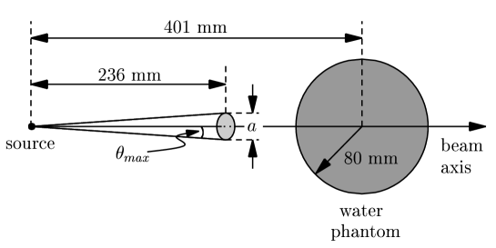
Figure 1: Schematic view of the simplified model of the source channel of the GK. A point source emits initial photons in a cone defined by itself and the apertures $a$, which are given in table 1. The water phantom used to simulate the patient head is also drawn.

Table 1: Apertures, $a$, and maximum polar angles, $\theta_{\rm max}$, of the emission cones for the initial photons in the simplified model of the source channel of the Leksell Gamma Knife^®. The values of the apertures correspond those of the helmet outer collimators and have been taken from Moskvin et al(2002).

Final beam diameter	4 mm	8 mm	14 mm	18 mm
$a$ [mm]	2.5	5.0	8.5	10.6
$\theta_{\rm max}$ [deg]	0.303	0.607	1.032	1.287

This simplified geometry has been considered for all the 201 source channels of the GK. Figure 2 shows a scheme of the situation of these sources. In the upper panel, the reference system we have considered is indicated. The origin of coordinates is situated at the isocenter of the GK and the $z$ axis is in the patient axis pointing from the head to the feet. The lower panel shows the disposal of the five rings in which the sources are distributed as well as the elevation angles of each one with respect to the isocenter plane. There are 44 sources in rings A and B, 39 in rings C and D and 35 in ring E. Table 2 shows the spherical coordinates of the 201 point sources. All of them have $r=401$ mm. On the other hand, the angles $\phi$ for each source in a given ring $\alpha$ are given by $\phi_{i}^{\alpha}=\phi_{1}^{\alpha}-i\Delta\phi^{\alpha}$, $i$ being the order label shown in the upper panel of figure 2.

Figure 2: Scheme of the situation of the 201 sources of the GK. The reference system used is indicated in the upper panel. Also the labeling of the sources is included. In the lower panel the elevation angles of the five rings in which the sources are distributed are shown.

Table 2: Spherical coordinates of the 201 point sources assumed in our calculations. We give the $\theta^{\alpha}$ coordinates of the five rings A to E in which the sources are distributed. The coordinates $\phi$ of each source are obtained as $\phi_{i}^{\alpha}=\phi_{1}^{\alpha}-i\Delta\phi^{\alpha}$, $i$ being the order label as shown in Fig. 2. All the sources have $r=40.1$ cm.

$\alpha$	A	B	C	D	E
$\theta^{\alpha}$ [deg]	96.0	103.5	111.0	118.5	126.0
$\phi^{\alpha}_{1}$ [deg]	266.25	266.0	261.0	255.5	260.0
$\Delta\phi^{\alpha}$ [deg]	7.5	8.0	9.0	9.0	10.0

It should be noted that the distribution of the sources in the rings is not completely uniform because some of them are not present (for example those labeled A₇, B₇, C₆, D₆, E₅, etc.) and this breaks the cylindrical symmetry of the system. Thus, the doses we have calculated depend on the three cartesian coordinates, $D(x,y,z)$. The scoring voxels we have used present $\Delta x=$0.5 mm and $\Delta y=\Delta z=1$ mm, for the 18 and 14 mm helmets, and $\Delta x=$0.25 mm and $\Delta y=\Delta z=$0.5 mm, for the 8 and 4 mm ones.

In connection with this point, we have studied the asymmetry between $x$ and $y$ axes, by calculating the quantity

$$A_{xy}(s)\,=\,\displaystyle\frac{D(s,0,0)-D(0,s,0)}{D(s,0,0)}\,,$$ (1)

and, also, the asymmetries between the negative and positive parts of the $x$ axis,

$$A_{x}(s)\,=\,\displaystyle\frac{D(s,0,0)-D(-s,0,0)}{D(s,0,0)}\,,s\geq 0\,,$$ (2)

and of the $y$ axis,

$$A_{y}(s)\,=\,\displaystyle\frac{D(0,s,0)-D(0,-s,0)}{D(0,s,0)}\,,s\geq 0\,.$$ (3)

In these calculations we have considered the configuration in which the 201 sources are unplugged. In addition, configurations with 150 and 102 sources have been considered. Figure 3 shows the corresponding plug patterns taken into account. Therein, the black circles represent the plugged sources.

Figure 3: Plug patterns for the configurations with 150 (left panel) and 102 (right panel) unplugged sources considered in this work. The black circles represents the plugged sources.

We have also calculated the dose output factors for the configuration with 201 sources. These are defined as the dose rate for a given collimator helmet, relative to that of the 18 mm helmet, at the isocenter, in presence of the phantom. To accumulate the energy, we have considered two kind of voxel centered at the isocenter. First, we have assumed a cubic voxel with dimensions $(2\Delta x,2\Delta y,2\Delta z)$, with $\Delta x$, $\Delta y$ and $\Delta z$ equal to the values given above for the scoring voxels. This corresponds to take the eight scoring voxels surrounding the isocenter as a unique voxel. Second, we have considered three spherical voxels with radii 0.5, 0.75 and 1 mm.

To calculate the output factors, the doses obtained have been renormalized to the case of a point source emitting isotropically,

$$D_{\rm norm}(x,y,z)\,=\,f_{\rm norm}\,D(x,y,z)\,,$$ (4)

where the normalization factor is

$$f_{\rm norm}\,=\,\displaystyle\frac{1-\cos\theta_{\rm max}}{2}\,,$$ (5)

with the corresponding $\theta_{\rm max}$ for each helmet.

2.2 Monte Carlo calculations

In this work we have used PENELOPE (v. 2001) (Salvat et al2001) to perform the calculations. PENELOPE is a general purpose MC code which permits the simulation of the coupled electron-photon transport. The energy range in which it can be applied goes from a few hundred eV up to 1 GeV, for arbitrary materials. PENELOPE describes in an accurate way the particle transport near interfaces.

PENELOPE performs analog simulation for photons and uses a mixed scheme for electrons and positrons. In this case, events are classified as hard (which are simulated in detail and are characterized by polar angular deflections or energy losses larger than certain cutoff values) and soft (which are described in terms of a condensed simulation based on a multiple scattering theory). Details can be found in Salvat et al(2001). The full tracking is controlled by means of five parameters. $C_{1}$, $C_{2}$, $W_{\rm cc}$, $W_{\rm cr}$ and $s_{\max}$. Besides the absorption energies for the different particles must be supplied. Table 3 shows the values we have assumed in our simulations for these parameters and for the two materials (air and water) present in the geometry.

Table 3: PENELOPE tracking parameters of the two materials assumed in our simulations. $E_{\rm abs}$($\gamma$) and $E_{\rm abs}$(e^-,e⁺) stand for the absorption energies corresponding to photons and electrons and positrons, respectively.

materials		Air	Water
$E_{\rm abs}$($\gamma$) [keV]		1.0	1.0
$E_{\rm abs}$(e-,e+) [keV]		0.1	50.0
$C_{1}$		0.05	0.1
$C_{2}$		0.05	0.05
$W_{\rm cc}$ [keV]		5.0	5.0
$W_{\rm cr}$ [keV]		1.0	1.0
$s_{\max}$ [cm]		$10^{35}$	$10^{35}$

Initial photons were emitted with the average energy 1.25 MeV. For each history in the simulation, a source was selected by sampling uniformly between the unplugged sources in the configuration analyzed. This determines the coordinates of the initial photon and the beam axis direction. Then the initial photon is emitted uniformly in the corresponding emission cone as defined in the simplified geometry.

The number of histories simulated has been chosen in each case to maintain the statistical uncertainties under reasonable levels. The uncertainties given throughout the paper correspond to 1$\sigma$.

Table 4: Composition of the materials assumed in the MC simulations performed in this work. The values correspond to the weight fraction of each element in the material. Also the densities are quoted.

	Air	Water
H		0.111894
C	0.000124
N	0.755267
O	0.231781	0.888106
Ar	0.012827
density [g cm-3]	0.0012048	1.0

The simulation geometry has been described by means of the geometrical package PENGEOM of PENELOPE. Table 4 gives the composition and densities of the two materials (air and water) assumed in our simulations.

To give an idea of the time needed to perform the simulations discussed below, we can say that it takes 11.2 minutes of CPU for each $10^{6}$ histories in a Origin 3400 of Silicon Graphics with a CPU R14000A at 600 MHz. In a PC with a CPU AMD Athlon XP 1800+ at 1600 Mhz the time needed is 16.6 minutes.

3 Results

In our first calculation, the configuration in which all the 201 sources are unplugged has been considered (see figure 2). A total of $15\cdot 10^{7}$ histories have been followed.

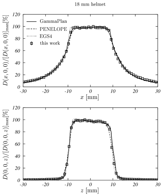
Figure 4: Dose profiles at the isocenter, relative to their respective maxima, in percentage, for the 18 mm helmet. Upper (lower) panel shows the results along $x$ ($z$) axis. Open squares are the results of our simulations. Dashed-dotted curves correspond to EGS4 results and have been obtained by scanning directly figures 4 and 5 of Xiaowei and Chunxiang (1999). Dashed curves have been obtained by Moskvin et al(2002) with PENELOPE for a polystyrene phantom. Solid curve corresponds to the predictions of GP quoted by Moskvin et al(2002). Both results have been obtained from figure 9 of Moskvin et al(2002).

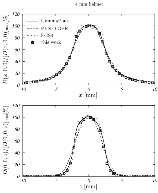
Figure 5: The same as in figure 4 but for the 4 mm helmet.

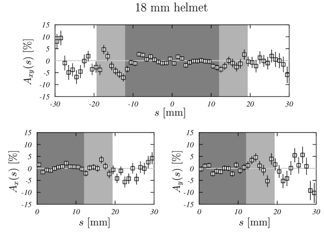
Figure 6: Asymmetries $A_{xy}$ (upper panel), $A_{x}$ (lower left panel) and $A_{y}$ (lower right panel), as given by equations (1), (2) and (3), in percentage, for the 18 mm helmet. The shadow areas mark the $s$ values for which the dose $D(s,0,0)$ is larger than 20% (clearer area) and 50% (darker area) of the maximum dose $[D(s,0,0)]_{\rm max}$.

Figures 4 and 5 show the dose profiles at the isocenter, $D(x,0,0)$ (upper panel) and $D(0,0,z)$ (lower panel), relative to their respective maxima, in percentage, for the 18 and 4 mm helmets, respectively. The results of our simulations (squares) are compared with those obtained with EGS4 by Xiaowei and Chunxiang (1999) (dotted curves), with PENELOPE (v. 2000) by Moskvin et al(2002) (dashed curves) and with the predictions of GP (Moskvin et al2002) (solid curves). The values quoted by Moskvin et al(2002) correspond to a polystyrene phantom.

For the 18 mm helmet (figure 4), we found a good agreement with the PENELOPE results of Moskvin et al(2002) and with those predicted by GP. Some differences with the calculation of Xiaowei and Chunxiang (1999) appear at the ending edges of the plateau of the maximum dose. For the 4 mm helmet (figure 5), the agreement with the GP predictions is rather good, while some discrepancies are observed with the other calculations, mainly for the $z$ profile (lower panel). Part of the disagreement with the PENELOPE results of Moskvin et al(2002) can be ascribed to the difference in the material forming the phantom (polystyrene in the case of these authors).

Due to lack of cylindrical symmetry shown by the source system of the GK, an interesting point to address concerns the asymmetry shown by the dose profiles. First, we have studied the asymmetry between $x$ and $y$ axes by means of $A_{xy}$ as given by equation (1). In the upper panel of figure 6, we show the values obtained for the 18 mm treatment helmet. The shadow regions indicate the $s$ values for which the corresponding dose $D(s,0,0)$ is larger than 20% (clearer) and 50% (darker) of the maximum dose, $[D(s,0,0)]_{\rm max}$. As we can see, the asymmetry is below 15% in absolute value for all $s$. This percentage reduces to around 5% and 2% in the two marked regions.

Also, we have determined for the same helmet, the asymmetries between the negative and positive parts of the $x$ axis, $A_{x}$ (see equation (2)) and of the $y$ axis, $A_{y}$ (see equation (3)). Results are plotted in the lower panels of figure 6, where the shadow regions have the same meaning mentioned above. Similar comments to those done for $A_{xy}$ can be stated in both cases. We have checked that the situation is the same for the remaining three helmets. The conclusion is that the loss of cylindrical symmetry in the GK, provoked by the absence of some source channels, has a rather slight effect on the dose profiles at the isocenter. These profiles show up cylindrical symmetry in practice.

As a second test of our simplified model, we have performed new simulations, in similar conditions to those of the previous configuration, but plugging 51 and 99 sources, as indicated in the schemes of figure 3.

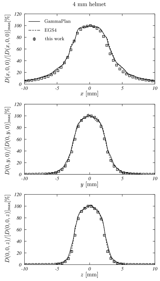
Figure 7: Dose profiles at the isocenter, relative to their respective maxima, in percentage, for the 4 mm helmet and for the configuration with 150 unplugged sources. The results along $x$, $y$ and $z$ axes are shown. Open squares are the results of our simulations. Dashed curves have been obtained by Cheung et al(1999a) with EGS4. Solid curve corresponds to the predictions of GP quoted by Cheung et al(1999a). Both results have been obtained by scanning directly figures 3-8 of Cheung et al(1999a).

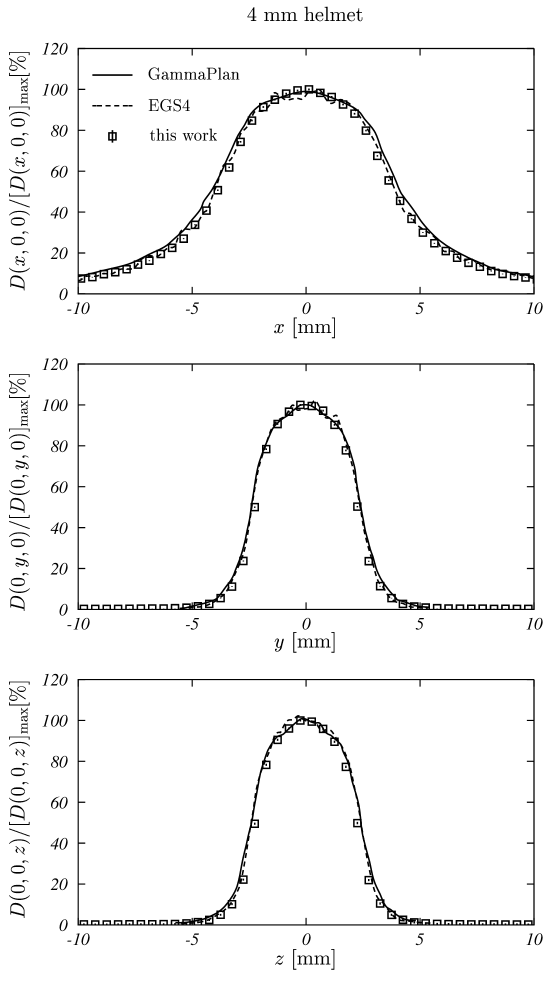
Figure 8: Same as in figure 7 but for the configuration with 102 unplugged sources.

In figures 7 and 8 we compare our results for the 4 mm helmet (squares) with those of Cheung et al(1999a) obtained with EGS4 (dashed curve) and with the GP predictions quoted by the same authors (solid curves). The three profiles along $x$ (upper panels), $y$ (medium panels) and $z$ (lower panels) axes are shown. As we can see, our results show a very good agreement with those obtained with EGS4. On the other hand, as in the case of the 201 source configuration, the agreement with the GP predictions is rather good.

As for the case of a single source (Al-Dweri et al(2004)), the simplified model of the source channel produces dose profiles which are in good agreement with other MC calculations and with the GP predictions. This ensures the feasibility of the simplified geometry model, which, in addition, permits a large reduction in the computation time (larger than a factor 15) with respect to the calculations with the full geometry.

Table 5: Comparison of the dose output factors quoted by different authors and obtained with MC simulations or measured with various techniques with those found in our calculations. The average value quoted by Tsai et al(2003) corresponds to a pool of measurements done with silicon diode, diamond detector, radiographic film, radiochromic film, and TLD cubes. The values of Moskvin et al(2002) were obtained with a spherical voxel of $R=$0.75 mm using a polystyrene phantom. The values we have obtained correspond to the cubic voxel described in the text (first row) and to spherical voxels with radii 0.5, 0.75 and 1 mm. In these three last cases a total of $2\cdot 10^{8}$ histories have been followed.

		14 mm	8 mm	4 mm
Elekta (1992)		0.984	0.956	0.800
Elekta (1998)				0.870
Cheung et al(1999b)	EGS4	0.974$\pm$0.009	0.951$\pm$0.009	0.872$\pm$0.009
	EGS4			0.876$\pm$0.005
	radiografic film			0.876$\pm$0.009
Ma et al(2000)	radiochromic film			0.870$\pm$0.018
	TLD			0.890$\pm$0.020
	Diode			0.884$\pm$0.016
Moskvin et al(2002)	PENELOPE
	$R=$0.75 mm	0.970$\pm$0.004	0.946$\pm$0.003	0.876$\pm$0.009
Tsai et al(2003)	average			0.868$\pm$0.014
this work	PENELOPE
	cubic voxel	0.982$\pm$0.007	0.967$\pm$0.007	0.876$\pm$0.006
	$R=$0.5 mm	0.99$\pm$0.03	0.95$\pm$0.03	0.86$\pm$0.03
	$R=$0.75 mm	0.99$\pm$0.02	0.96$\pm$0.02	0.86$\pm$0.01
	$R=$1 mm	0.978$\pm$0.009	0.950$\pm$0.008	0.846$\pm$0.006

Finally, we have calculated the dose output factors for the configuration with 201 sources. First, we have performed the calculations using the cubic voxel described in section 2.1. In table 5 we compare the results we have obtained (see first row labeled “this work”) with those found by other authors by means of MC simulations or different measurement procedures. Our results are in good agreement with the findings of the other authors in case of the 4 mm helmet. The value we have obtained for the 8 mm helmet agrees within the statistical uncertainties with the one quoted by Cheung et al(1999b), but it is noticeably larger than those of Elekta (1992) and Moskvin et al(2002). Finally, for the 14 mm helmet, our result agrees with those of Cheung et al(1999b) and the manufacturer (Elekta 1992), but differs (at the 1$\sigma$ level) from that of Moskvin et al(2002).

Out of the discrepancies noted, the most significant are those found with the calculations of Moskvin et al(2002). These authors have used the version 2000 of PENELOPE code, but the differences between this version and the 2001 we have used are not expected to produce such discrepancies. This is corroborated by the good agreement we have found when comparing the dose profiles discussed above.

In order to clarify this disagreement, we have investigated if it is due to differences in the scoring voxels chosen for the calculations. Moskvin et al(2002) considered a spherical voxel with radius 0.75 mm. Thus we have performed new simulations, following $2\cdot 10^{8}$ histories, and using the spherical voxels described in section 2.1. The results are shown in the last three rows of table 5. As we can see, there are not significant variations (within the statistical uncertainties) when the radius of the voxel is reduced. On the other hand, the results obtained for these spherical voxels are into agreement with the values quoted by Moskvin et al(2002). This points out a dependence of the dose output factors with the shape of the scoring voxel.

4 Conclusions

In this work we have investigated the dosimetry of the GK by considering a simplified model for the single source channels. Calculations have been done by using the Monte Carlo code PENELOPE (v. 2001) for different configurations including 201, 150 and 102 unplugged sources.

The use of the simplified model produce results for the dose profiles at the isocenter which are into agreement with previous calculations done with other MC codes and with the predictions of the GP. The absence of cylindrical geometry due to the lack of some source channels in the GK does not show up in the calculated dose profiles.

Besides, we have determined the dose output factors corresponding to the 14, 8 and 4 mm helmets. The results found show a good agreement with those obtained with EGS4 and measured by means of different procedures, mainly for the 4 mm helmet. The discrepancies observed with previous results obtained also with PENELOPE are largely reduced once one uses scoring voxels with the same shape. This voxel shape dependence deserves a deeper investigation which we are carrying out at present.

The results quoted here, together with those found for the single source configuration (Al-Dweri et al2004), prove the suitability of the simplified geometry proposed to perform dosimetry calculations for the GK. The simplicity of this model and the level of accuracy which can be obtained by using it opens the possibility to use MC tools for planning purposes in the GK, mainly if we take into account the reduction in the computational time (around a factor 15) with respect to the full geometry simulations. As an additional gain, MC simulations permit to take into account the presence of inhomogeneities and interfaces in the target geometry, which are not correctly treated by GP.

References

References

- [1]
- [2] [] Al-Dweri F M O, Lallena A M and Vilches M 2004 A simplified model of the source channel of the Leksell Gamma Knife® tested with PENELOPE Phys. Med. Biol. 49 2687-2703
- [3]
- [4] [] Cheung J Y C, Yu K N, Ho R T K and Yu C P 1999a Monte Carlo calculations and GafChromic film measurements for plugged collimator helmets of Leksell Gamma Knife unit Med. Phys. 26 1252-6
- [5]
- [6] [] Cheung J Y C, Yu K N, Ho R T K and Yu C P 1999b Monte Carlo calculated output factors of a Leksell Gamma Knife unit Phys. Med. Biol. 44 N247-9
- [7]
- [8] [] Cheung J Y C, Yu K N, Ho R T K and Yu C P 2000 Stereotactic dose planning system used in Leksell Gamma Knife model-B: EGS4 Monte Carlo versus GafChromic films MD-55 Appl. Radiat. Isot. 53 427-30
- [9]
- [10] [] Cheung J Y C, Yu K N, Yu C P and Ho R T K 1998 Monte Carlo calculation of single-beam dose profiles used in a gamma knife treatment planning system Med. Phys. 25 1673-5
- [11]
- [12] [] Cheung J Y C, Yu K N, Yu C P and Ho R T K 2001 Dose distributions at extreme irradiation depths of gamma knife radiosurgery: EGS4 Monte Carlo calculations Appl. Radiat. Isot. 54 461-5
- [13]
- [14] [] Elekta 1992 Leksell Gamma Unit-User’s Manual (Stockholm: Elekta Instruments AB)
- [15]
- [16] [] Elekta 1996 Leksell GammaPlan Instructions for Use for Version 4.0-Target Series (Geneva: Elekta)
- [17]
- [18] [] Elekta 1998 New 4-mm helmet output factor (Stockholm: Elekta)
- [19]
- [20] []Ma Ma L, Li X A and Yu C X 2000 An efficient method of measuring the 4 mm helmet output factor for the Gamma Knife Phys. Med. Biol. 45 729-733
- [21]
- [22] [] Moskvin V, DesRosiers C, Papiez L, Timmerman R, Randall M and DesRosiers P 2002 Monte Carlo simulation of the Leksell Gamma Knife: I. Source modelling and calculations in homogeneous media Phys. Med. Biol. 47 1995-2011
- [23]
- [24] [] Salvat F, Fernández-Varea J M, Acosta E and Sempau J 2001 PENELOPE, a code system for Monte Carlo simulation of electron and photon transport (Paris: NEA-OECD)
- [25]
- [26] [] Tsai J-S, Rivard M J, Engler M J, Mignano J E, Wazer D E and Shucart W A 2003 Determination of the 4 mm Gamma Knife helmet relative output factor using a variety of detectors Med. Phys. 30 986-992
- [27]
- [28] [] Xiaowei L and Chunxiang Z 1999 Simulation of dose distribution irradiation by the Leksell Gamma Unit Phys. Med. Biol. 44 441-5
- [29]