The measurements of 2200 ETL9351 type photomultipliers for the Borexino experiment with the photomultiplier testing facility at LNGS.

Abstract

The results of tests of more than 2200 ETL9351 type PMTs for the Borexino detector with the PMT test facility are presented. The PMTs characteristics relevant for the proper detector operation and modeling are discussed in detail.

A.Ianni, P.Lombardi, G.Ranucci², and O.Smirnov

1 Introduction

The Borexino detector is a large volume liquid scintillator detector designed especially for detection of Solar ${}^{7}Be$ neutrino [1]. The scintillation from the recoil electrons is registered by 2200 8” PMTs surrounding the detector’s active volume. All PMTs before installation in the detector were carefully tested in the specially designed test facility. The technical description of the PMT test facility at Gran Sasso for the Borexino experiment is presented in another paper [2]. Here we discuss in detail the most important PMT characteristics measured during the tests. The measured characteristics split naturally into 4 classes:

1. Dark noise measurements (using scalers);

2. Charge spectrum measurements (using charge amplitude-to-digital converters, ADC);

3. Transit time timing measurements on the short time scale of 100 ns (using time-to-digital converters (TDC) with 250 ps resolution);

4. Afterpulses timing measurements on the long time scale of 30 $\mu$s (using Multihit TDCs with 1 ns resolution).

In this paper the detailed description of the results of measurements for each of the 4 classes is given. The set of characteristics for the PMT, which passed the acceptance test was put into the database prepared for the experiment, but because of the huge amount of PMTs used in the detector, the straightforward use of the database for the detector’s modeling would slow down the calculations. Therefore, for the purpose of the detector modeling, the average characteristics of the PMTs for each class of measurement have been determined.

2 Dark noise

In order to minimize the probability of the random trigger in the detector, the PMTs with a high dark noise rate were rejected. Another drawback of the high dark noise rate is the shift of the energy scale of the detector by the amount of the random charge collected during the event window. The technical specification for the factory was set at the maximum level of 20000 counts per second (cps). Tests showed that the initial dark rate is decreasing exponentially during 3-4 hours, then it is still decreasing but much slower, with a characteristic time of up to 50 days. The typical example of the dark rate behaviour during a 3 days run is shown in Fig.1. It should be noted that this is mainly thermoelectron noise and correlated with it ionic/dynodes afterpulsing (at the level of $\simeq 5\%$).

The other components of the dark rate, namely signals induced by high energy cosmic rays and by natural radioactivity, are negligible. Furthermore, at the underground site of the Gran Sasso laboratory (built at a depth of 3500 meters of water equivalent) the cosmic muon flux is reduced by a factor $10^{6}$. As concerning the natural radioactivity of the PMT components, very strong limits on the content of the radioactive elements from the $U-Th$ chains, and potentially very dangerous ${}^{40}K$ in the glass of the PMT bulb, were set for the manufacturer.

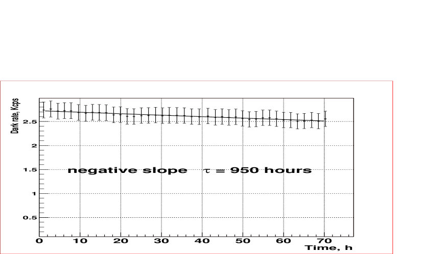
Figure 1: Dark rate of the ETL ser.No 5797.

Some of the PMTs demonstrate a very rapid decrease of dark rate, an example of such behaviour is demonstrated in Fig.2. The dark rate of the PMT has been changed by one order of magnitude after 1 day under dark conditions. Very probably this behaviour reflects some constructive peculiarities of the PMT. Usually, the dark rate after 3-4 hours was small enough to allow the starting of measurements. PMTs with a high dark rate noise were kept in the dark for much longer periods in order to exclude the possibility of rejection of devices with acceptable dark rate in stable regime. It should be noted that the dark rate measured at the test facility is usually a factor 2-3 higher than the dark rate at operating conditions in the detector, due to the much higher time of deexcitation and lower temperature at the underground site. An example of the dark rate behaviour in time for a PMT that does not demonstrate dark rate stabilization is presented in Fig.3.

The dark rate of each PMT has been measured every 10 minutes during the test. The results for 2000 PMTs are presented in Fig.4.

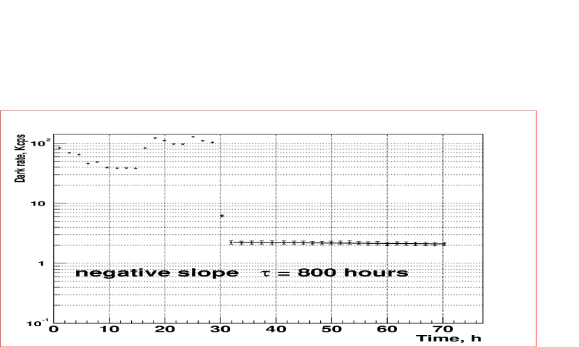
Figure 2: Dark rate of the ETL ser.No 5832.

It is a well-known fact that the dark rate of the PMTs shows significant deviations from Poisson statistics. In order to estimate the stability of the dark rate count we used the excess variation over the Poisson statistics:

$$S=\frac{\sqrt{<f_{dark}^{2}>-<f_{dark}>^{2}}}{<f_{dark}>}.$$

In the case of normal (or Poissonian) statistics of the dark rate measurements the variable $S$ should be close to unity. For the PMTs with a low dark rate (about 1 Kcps) left for a long period (at least 1 week) under dark conditions the stability $S$ was in a range of 1.2-1.5. The effect of the very slow decrease of the dark rate can be due to the slow variation of the average ambient temperature (for the same reason the $S$ factor is greater than 1 even for the very stable PMTs).

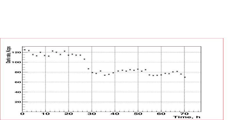
Figure 3: Dark rate of the ETL ser.No 5812.

In the bulk measurements the PMTs were kept in the dark only for the period necessary for the decay of the fast component of the dark rate (3-4 hours). The decrease of the dark rate during the measurements was the main source of the bigger values of the parameter $S$. The statistics of the parameter $S$ over the measured sample of 2300 PMTs is shown in Fig.5 (upper plot). One can see that high values of $S$ , up to 50 and even more, were observed. A strong correlation between the PMT dark rate and the parameter $S$ exists. The lower plots in Fig.5 represent parameter $S$ for the PMTs with low dark rate $f<1$ Kcps, and for the PMTs with high dark rate $f>10$ Kcps. It is clearly seen the increase of the relative variance of the dark rate for the PMTs with higher dark rate.

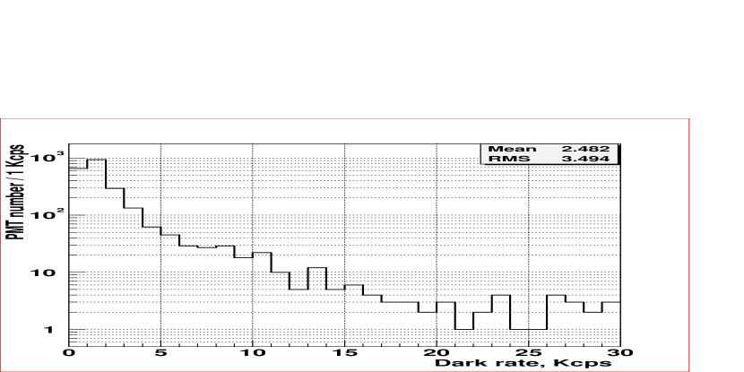
Figure 4: Statistics of the dark rate

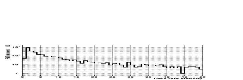
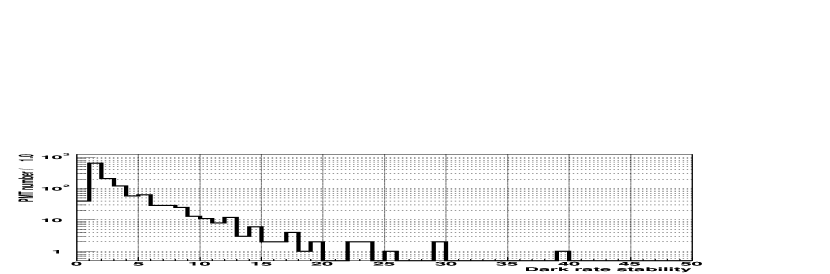
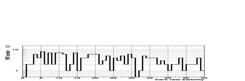
Figure 5: From up to down: stability, S, of the dark rate for all PMTs, S for the PMTs with low dark rate f<1 Kcps, and for the PMTs with high dark rate f>10 Kcps.

3 Charge spectrum

3.1 Charge spectrum structure

The charge spectra of the 8” ETL9351 series were studied at our test facility before the bulk test of the PMTs start. The results were presented in [3], where a simple phenomenological model was proposed to describe the data. In particular, it was shown that the single photoelectron amplitude spectrum of the PMT consists of two main contributions. The main contribution (>80% of all signals) is described with a Gaussian distribution; the remaining $\simeq 20\%$ of signals are underamplified and can be described by an exponential distribution with a negative slope. Examples of various charge spectra are shown in Fig.6 (PMT with a poor resolution) and Fig.7 (PMT with a good resolution).

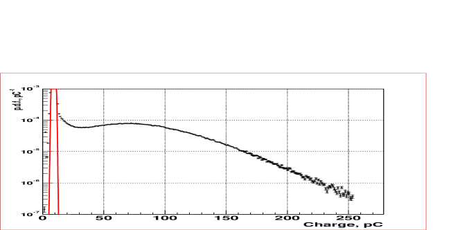
Figure 6: Example of the charge spectrum of the PMT with a poor peak-to-valley ratio ($p/V=1.35$ and $v_{1}=0.3$).

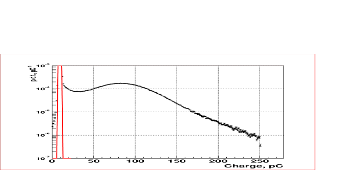
Figure 7: Example of the charge spectrum of the PMT with a high peak-to-valley ratio ($p/V=2.27$ and $v_{1}=0.46$).

The data of the charge spectra for 2200 PMTs were averaged in order to obtain a typical response of the photomultiplier. The procedure of spectra averaging consisted of the following steps:

1. The position of the pedestal in the charge spectrum is found and the histogram is shifted in order to put its pedestal at the position corresponding to $q=0$. The histogram is normalized to 1.

2. All the histograms are summed together and normalized to 1 once more. The obtained histogram contains the mean characteristics of a sample of the PMTs used with a pedestal position at $q=0$.

An ideal single electron charge response model consisting of a Gaussian and an exponential has been used to fit the experimental data ([3]):

$$SER_{0}(q)=\left\{\begin{array}[]{cc}\frac{p_{E}}{A}e^{-\frac{q-q_{p}}{A}}+\frac{1}{\sqrt{2\pi}\sigma_{0}}\frac{1-p_{E}}{g_{N}}e^{-\frac{1}{2}(\frac{q-q_{0}-q_{p}}{\sigma_{0}})^{2}},&q>q_{p}\\ 0,&q\leq q_{p}\end{array}\right.$$ (1)

with the following parameters:

- $A$ is the slope of the exponential part of the $SER_{0}(q)$

- $p_{E}$ is the fraction of events under the exponential function,

- $q_{p}$ is the pedestal position,

- $q_{0}$ and $\sigma_{0}$ the mean value and the standard deviation of the Gaussian part of the single p.e. response respectively;

and the factor

$$g_{N}=\frac{1}{2}\Big{(}1+Erf\Big{(}\frac{q_{0}}{\sqrt{2}\sigma}\Big{)}\Big{)}$$

takes account for the cut of the Gaussian part of the PMT response.

To account for the electronics noise one should perform the convolution of the ideal SER with a noise function, $Noise(x)$ :

$$SER(q)=SER_{0}(q)\otimes Noise(q),$$

where:

$$Noise(q)=\frac{1}{\sqrt{2\pi}\sigma_{p}}e^{-\frac{1}{2}(\frac{q-q_{p}}{\sigma_{p}})^{2}},$$

which fits the pedestal with a proper normalization. The convolution does not influence the Gaussian part of the SER since $\sigma_{1}>>\sigma_{p}$ (in our measurements $\sigma_{p}\sim 0.01\sigma_{1}$), but it does affect the exponential one which is closer to the pedestal. The analytical formula for the convolution of the exponential function with the Gaussian is:

$$\frac{p_{E}}{2A}\cdot e^{\frac{\sigma_{p}^{2}-2A(q-q_{p})}{2A^{2}}}\cdot(1+Erf(\frac{A(q-q_{p})-\sigma_{p}^{2}}{\sqrt{2}A\sigma_{p}})),$$

where $Erf(q)$ is the error function.

The PMT response for a low light intensity contains a certain amount of multiple primary p.e. signals. Assuming the linearity of the PMT response, one can write: $q_{n}=nq_{1}$ and $\sigma_{n}=\sqrt{n}\sigma_{1}$, where $q_{n}$ and $\sigma_{n}$ are the mean value and the standard deviation of the PMT response to n p.e., respectively. Taking into account the Poisson distribution of the detected light and using a Gaussian approximation for the responses to $Np.e.>2$, the multi-p.e. response will have the following form:

$$M(q)=\sum_{n=2}^{N_{M}}\frac{P(n;\mu)}{\sqrt{2n\pi}\sigma_{1}}e^{-\frac{1}{2n}(\frac{q-nq_{1}-q_{p}}{\sigma_{1}})^{2}}$$ (2)

where the response to n p.e. is approximated by a Gaussian and $P(n;\mu)$ is the Poisson distribution with mean value $\mu$ to account for the different contributions of $0\rightarrow n$ p.e. In (2) $N_{M}$, the maximum number of multiple-p.e. responses considered, depends on $\mu$ and on the ADC scale. The function $M(q)$ has three additional parameters $\mu$, $q_{1}$ and $\sigma_{1}$.

The approximate values of $q_{1}$ and $\sigma_{1}$ can be calculated from (1):

$$q_{1}\approx(1-p_{E})\cdot q_{0}+p_{E}A$$

$$\sigma_{1}^{2}\approx(1-p_{E})\cdot(\sigma_{0}^{2}+x_{0}^{2})+2p_{E}A^{2}-q_{1}^{2}.$$

The approximate character of these formulae come from the cut in the Gaussian part of the SER, whose portion below 0 is truncated.

The final fitting function for the PMT spectrum can be written as:

$$f(x)=N_{0}\cdot(P(0)\cdot Noise(x)+P(1)\cdot SER(x)+M(x))$$ (3)

where $N_{0}$ is a normalization factor.

A certain distortion of the spectra is expected due to the different PMTs illumination, sensitivity and amplification. All the electronics channels were carefully calibrated in order to provide exact knowledge of the amplification of the channel and the high voltage of the PMTs were adjusted with a precision of better than $2\%$ [2, 5]. Thus, the main expected source of the spectrum distortions is due to the effect of different PMT mean counts. The mean photoelectrons count was checked during the tests with a high precision, the results are presented in Fig.8. In order to account for the distortions of the spectrum due to the variations of the mean photoelectron count, the Poisson probabilities of formula (3) were transformed using the rule:

$$P_{exp}(N)=\int_{0}^{N_{max}}P(N,\mu)F_{\mu}(\mu)d\mu,$$

with $N_{max}\simeq 10$, which is big enough for the mean count of $\mu=0.05$ p.e. and $F_{\mu}(\mu)$ is the measured distribution of the mean photoelectrons count (see Fig.8). A Gaussian distribution was used as an approximation of $F_{\mu}(\mu)$.

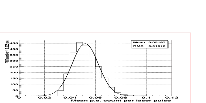
Figure 8: mean photoelectrons count per laser pulse. The Gaussian fit is superimposed with the parameters practically coinciding with the mean and r.m.s. value for the histogram.

The results of the fit are presented in Fig.9 and the parameters are given in Table.1. It should be noted that parameters $q_{1}$ and $\sigma_{1}$ are not independent. The value of $q_{1}$ was used to calibrate the scale in p.e., thus $q_{1}=1.00$ by definition.

parameter	$q_{0}$	$\sigma_{0}$	A	$p_{U}$	$\mu$	$q_{1}$	$\sigma_{1}$
value	1.16 p.e.	0.52 p.e.	0.19 p.e.	0.18	0.059 p.e.	1.00 p.e.	0.58p.e.

Table 1: The parameters of the charge spectrum fit

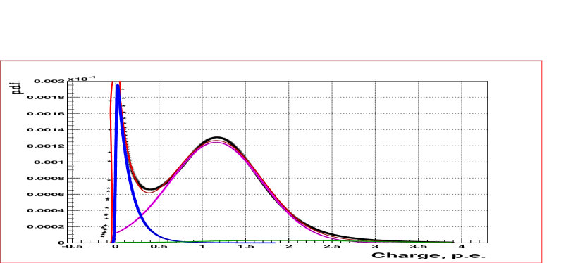
Figure 9: The fit of the average charge spectra of the PMT.

The mechanism of the electron multiplication allows to extract the gain on the first PMT dynode $g_{1}$. First, we note that the variance of the normally multiplied PMT signal (i.e. the part of the charge spectrum corresponding to a Gaussian contribute for which $v(M)\equiv v_{0}=(\frac{\sigma_{0}}{q_{0}})^{2}$) should satisfy the relation for the cascade processes (see i.e.[8]):

$$v(M)=v(g_{1})+\frac{v(g_{2})}{g_{1}}+\frac{v(g_{3})}{g_{1}g_{2}}+...,$$ (4)

where $M$ is total multiplication of the 12-stages dynode system, $g_{1}$ is the mean electron multiplication factor on the first dynode, $g_{2}$- on the second, etc. The divider used provided equal voltage on the last 9 stages of multiplication $U_{D}$, double voltage on the second stage of multiplication, and $1.5U_{D}$ on the third one. If $U_{D}$ is small enough to ensure the linearity of the multiplication in the region up to $2U_{D}$, then $g_{2}=2\cdot g$ and $g_{3}=1.5\cdot g$, where $g$ is the mean amplification on each of the remaining dynodes. In the case of the Poisson variances of the electron multiplication $v(g_{1})=\frac{1}{g_{1}}$, $v(g_{2})=\frac{1}{g_{2}}$ etc., and (4) reduces to:

$$v_{0}\equiv(\frac{\sigma_{0}}{q_{0}})^{2}=\frac{1}{g_{1}}\cdot\frac{6g^{2}-3g-1}{6g(g-1)}.$$ (5)

The mean gain of the multiplier is set to $M=2\times 10^{7}$, and the overall gain of the multiplier is the product of the gains at each stage: $M=3g_{1}g^{11}$ (on the last stages of the electron multiplier the gain can be reduced because of the spatial charge effect, as it was noted in [5], but it is of no significance for our calculations), and we have a system of two equations with two variables. Because of the 11-th degree in the equation for $g$ it is practically independent of $g_{1}$and lies in the region $3.6<g<3.3$ for $5<g_{1}<15$. The estimation of $g_{1}$ for 2000 PMTs is presented in Fig.10, in Fig.11 is presented the relative variance of the single electron charge spectrum in dependence on the gain on the first dynode. One can see, that the overall performance of the PMT depends on the gain on the first dynode. The average value of $v_{1}=0.34$ corresponds to the quite low mean values of $g_{1}=4-6$. This value is much less than expected for the type of the material used at the high voltage applied. Probably, this is the effect of the different conditions during the multiplication coefficient measurements, in which the incidence angle of the primary electrons is fixed, and the operational conditions in the PMT, when the angle of incidence is varying in a wide interval, and the effective gain is a result of averaging over all possible angles of incidence. Using the value $g=3.56$ (for $g_{1}=5.7$) one can write an approximate formula for the estimation of $g_{1}$ from the relative width of the main peak at the s.e.r. spectrum: $g_{1}\simeq\frac{1.18}{v_{0}}$.

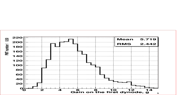
Figure 10: The statistics of the mean electrons gain on the first dynode, $g_{1}$

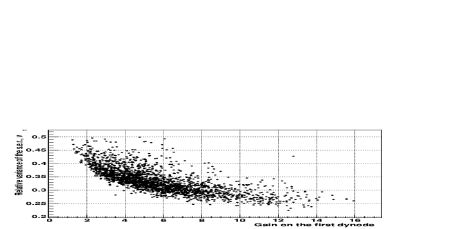
Figure 11: Relative variance of the single electron charge spectrum in dependence on the gain on the first dynode.

The relatively big amount of the small amplitude pulses is due to the fact that all the events in the 60 ns window are processed. As it will be discussed below, there is a notable amount of small amplitude pulses which arrives with a delay in respect to the main pulse. They correspond to the inelastic scattering of photoelectron on the first dynode. A special measurement was performed with a selection on the arrival time, showing the decrease of the contribution of the small amplitude pulses for the event arriving in time interval $t_{0}\pm\sigma_{t}$. The advanced study of the time-amplitude characteristics of the PMTs is now in progress, the results will be presented elsewhere.

It should be noted that the model fails to describe the s.e.r. in all details. Though the response to the more intense light sources with $\mu\simeq 1$ is fitted well [3], the very high statistics of the data allows to see the deviations from the model. One can note three features of the model in comparison to the experimental data: 1) the underfilled valley region between the main peak and the pedestal; 2) the lower peak value of the model; 3) the tail of the model is almost a factor 2 lower than the experimental data. The last feature is a consequence of the Poisson statistics of the multiplication on the first dynode. If one takes into consideration the mean value of $g_{1}\simeq 5.7$, then it is easy to check that at the position corresponding to $>2\times g_{1}$ primary electrons the Poisson distribution has factor 2 higher tail. The mean gain for the underamplified branch should correspond to the value $1/g_{1}$ in the case when a primary electron loses all its energy on the first dynode in inelastic scattering. One can see that the parameter $A=0.19$ p.e. from Table 1 is very close to the value $0.2$, that can be obtained dividing the mean amplification for a Gaussian part of the s.e.r. spectrum $q_{0}=1.16$ by the mean value of the $g_{1}$ coefficient $g_{1}=5.7$ (see below). This fact confirms that the major part of the underamplified signals are produced in totally inelastic scattering of the photoelectron on the first dynode.

3.2 Charge spectrum characterization

The PMT charge resolution is characterized by the manufacturer by the peak-to-valley ratio. The measured peak-to-valley ratio is presented in Fig.12.

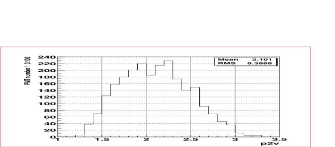
Figure 12: Peak-to-valley ratio

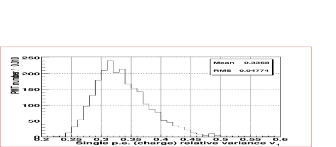
Figure 13: Relative variance of the single p.e. response

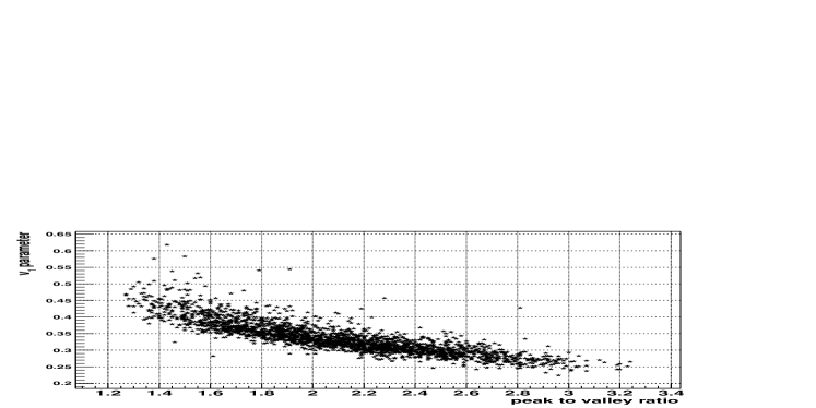
Figure 14: Relative variance of the single p.e. response versus peak to valley ratio.

For the numerical estimation of the detector resolution this parameter has no immediate significance. More informative is the relative resolution of the single photoelectron charge spectrum $v_{1}\equiv\frac{\sigma_{1}^{2}}{q_{1}^{2}}$. As it was shown in [4] the relative charge resolution of the detector with a spherical symmetry in the regime of the total charge measurement can be related to the average relative resolution of the single photoelectron charge spectrum $\overline{v_{1}}\approx\frac{1}{N_{PM}}\sum v_{1_{i}}$:

$$R=\sqrt{\frac{\sigma_{Q}^{2}}{Q^{2}}}=\sqrt{\frac{1+\overline{v_{1}}}{Q_{0}(E)<f_{s}>_{V}}+v(f_{s})}\>.$$ (6)

with constant parameters $v(f_{s})$ and $<f_{s}>_{V}\simeq 1$ characterizing the detector. The parameters $v_{1}$ and peak-to-valley ratio are correlated, as it can be seen in Fig.14, where the relative variance of the single p.e. response is plotted versus the peak-to-valley ratio.

The statistics of the measured values of parameter $v_{1}$ is presented in Fig.13. The relative single photoelectron charge variance averaged over all accepted PMTs turns out to be $\overline{v_{1}}\approx 0.34$. The mean relative variance of the Gaussian part of the s.e.r. is much less, $\overline{v_{0}}=0.24$ (see Fig.15). The presence of the exponential branch in the s.e.r. is the reason of such a resolution degradation. The relative strength of the exponential branch (underamplified signals fraction) is presented in Fig.16.

Figure 15: The mean relative variance of the Gaussian part of the s.e.r.

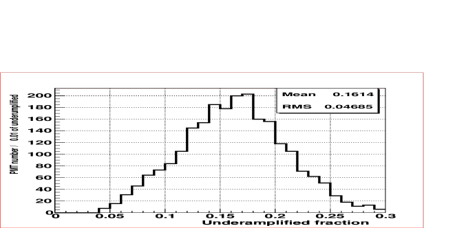
Figure 16: The fraction of the exponential branch

4 Transit time

4.1 Time spectrum structure

The most important characteristics of the time spectrum are the variance of the main peak in the spectrum, the relative amount of the late pulses and the relative amount of the prepulses.

The details of the transit time spectrum of the 8” ETL9351 series were studied in [6] using the results of the bulk tests. The spectra of 2200 PMTs were used to produce an averaged time spectrum. Because every PMT operates at its own voltage, and the lighting conditions depends on the position on the test tables, the procedure of averaging should be preceded by equalizing the difference in the measurement conditions. In [6] it was shown that the probability density function of the single photoelectron time arrival can be calculated as:

$$N_{1}(i)=\frac{1}{\mu}\frac{N_{Exp}(i)}{1-s\;(i)},$$ (7)

where

$$s\>(i)\equiv\frac{1}{N_{Triggers}}\sum_{k=1}^{k=i}N_{Exp}(k)$$ (8)

is the running sum of the histograms of the experimental data $N_{Exp}(i)$ normalized by the number of the system starts $N_{Triggers}$. For $N_{Triggers}$ large enough $s\>(\infty)=1-e^{-\mu}$.

The procedure of spectra averaging consisted in the following steps:

1. Using the measured value of the dark rate, the contribution $N_{dark}$ of the random coincidences at one bin was calculated.

2. Using equations (7) and (8) with $N_{exp}(i)$ substituted by $N_{exp}(i)$-$N_{dark}(i)$, the $N_{1}(i)$ function was calculated and normalized:

   $$n_{1}=\frac{N_{1}(i)}{\sum_{i=1}^{N_{bins}}N_{1}(i)}.$$ (9)

3. The peak in the distribution $n_{1}$ is found and the histogram is shifted in order to put its maximum at the position corresponding to $t=0$.

4. All the histograms are summed together and normalized to 1 once more. The obtained histogram contains the mean characteristics of a sample of the PMTs used with a peak (not mean time of the arrival) at the position $t=0$.

The resulting histogram is presented in Fig.17. This is the PMT transit time p.d.f. averaged over a 2200 PMT sample. The spectrum corresponds to an average level of the discriminator of $0.17$ p.e. The structure of the photomultiplier transit time exhibits the following main features: 1) an almost Gaussian peak at the position $t=0$ ns; 2) a very weak peak at $t=-24$ ns; 3) a weak peak at $t=48$ ns; 4) the continuous distribution of the signals arriving between the main peak and the peak at $t=48$ ns; and 5) another very weak peak at $t=20$ ns.

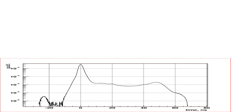
Figure 17: The averaged timing characteristics of the ETL9351 PMT.

Below we summarize briefly the results of the study of these features performed in [6]. A small peak at about -24 ns is a result of direct photoproduction of the electron on the first dynode. The amplitude of these pulses is a factor $g_{1}$(amplification of the first dynode) lower then the amplitude of the main peak. Because a typical value is $g_{1}\simeq 5.7$, these pulses are strongly suppressed by the discriminator threshold set at the 0.2 p.e. level. The shape of the peak is well approximated by a Gaussian one with a total intensity of $1.22\cdot 10^{-4}$. ˙This corresponds roughly to the ratio of the surfaces of the photocathode $S_{PMT}$ and the first dynode $S_{D_{1}}$. One can write the relative probability of the photoelectron production at the first dynode assuming the same efficiency of the photoproduction at the photocathode and the first dynode as:

$$p=\frac{S_{D_{1}}}{S_{PMT}}\cdot\tau\cdot r\cdot e^{-\frac{th}{1/g_{1}}},$$

where $\tau$ is transparency of the photocathode; $r$ is the ratio of the quantum efficiencies on the first dynode and on the photocathode, and $th$ is the threshold of the detection (in assumption of the exponential distribution of the amplitudes of prepulses). An estimation with $\tau=0.5$, $th=0.17$ p.e., $r=1$ and $g_{1}=5.7$ gives $p\simeq 1.5\cdot 10^{-4}$ which is in agreement with the measured value.

The difference $dt=23.2$ ns between the position of the main peak $t_{0}$, and the position of the prepulses peak $t_{pp}$ corresponds to the drift time of the electron from the photocathode to the first dynode $t_{d}$ with the time of flight of photon to the first dynode $t_{tof}$ subtracted: $dt=t_{0}-t_{pp}=t_{d}-t_{tof}$ . The time of flight can be calculated from the known distance between the photocathode and the first dynode, which is 123 mm (radius of the spherical photocathode is 110 mm, the focusing grid is situated at the center of the sphere, the distance between the focusing grid and the first dynode is 13 mm). Hence the time of flight of photon inside the PMT is $tof=0.4$ ns, and the drift time $t_{d}=dt+tof=23.6$ ns. The drift time is the same for all the PMTs tested, because the potential difference between the photocathode and the first dynode is stabilized.

In setups with a large number of PMTs in use, such as the Borexino detector, the presence of prepulses is a potential source of early triggers of the system. With a total number of the 2000 PMTs and the light yield of 400 p.e./MeV, the probability of early trigger for an event of 500 keV is about $2.5\%$.

The peak with probability $p_{r}=5.8\cdot 10^{-4}$ at $t=20.2$ ns corresponds to the electron’s transit time from the photocathode to the focusing grid and is caused by light feedback on the accelerating dynode. The spread of the peak $\sigma=1.07$ ns coincides with the main peak spread.

Pulses arriving with a delay relative to the main pulse in the time spectrum are called late pulses. The position of the last peak helps in clarifying its origin. The difference between the position of the last peak and the main peak is $\Delta t=47.6$ ns, and it coincides with a double drift time $2t_{d}=47.2$ ns. The double drift time can be explained by electrons which elastically backscatter on the accelerating grid, then go away from it, slow down and stop near the photocathode, and then are accelerated back to the first dynode to produce a signal. Two experimental facts are confirming this conclusion. First, the position of the last peak depends on the applied voltage, in the case of the backscattering on the first dynode the drift time should be constant because the potential of the first dynode is stabilized. The second argument is the geometry of the PMT dynode system entrance. The first dynode is designed to scatter electrons by 90^∘ angle. The elastically scattered photoelectrons should be transferred to the second dynode with a higher speed [7], producing small amplitude pulses preceding the main one. This phenomena was indeed observed in our measurements (see [6]), and we called it early pulsing.

The amplitude spectrum of these pulses is very similar to that of the main peak pulses. The total probability to observe photoelectron elastically scattered on the accelerating electrode is $0.024$.

The shape of the main pulse has significant deviations from the Gaussian shape not only in the region $t<t_{0}$, but in the region $t>t_{0}$, as well. The distortions of the shape close to the main peak position are due to the registering of the photons scattered inside the PMT. The typical delay time of this signals is of the order of 1 ns.

The remaining contribution to the late pulses corresponds to an inelastic scattering of the photoelectron on the first dynode, without any secondaries produced. In this case, part of initial energy of the incident electron is dissipated as heat in the material of the dynode, and the drift time of the electron in this case depends on the remaining part of the energy, and, naturally, is less than in the case of elastic scattering. In the extreme case all the energy is dissipated, and, without any delay, the electron is transferred to the next stage of amplification, producing on the average a signal with an amplitude of factor $g_{1}$ smaller than a normal signal. In the intermediate case, the scattered electron is delayed by a time in the range $0-2t_{d}$, and after returning back to the first dynode produces a signal with lower amplitude in comparison to the amplitudes of the main peak signals. The smaller the delay, the smaller is the amplitude of the signal. The total probability of inelastic scattering of photoelectrons is $0.038$.

4.2 Time spectrum Characterization

The characteristic of main concern is the width of the main peak in the transit time spectra. The results of measurements are presented in Fig.18. The width of the peak was defined by fitting the main peak region with a Gaussian distribution.

As it was noticed above, the prepulses corresponding to the direct photoproduction on the first dynode have a negligible probability due to the small size of the first dynode in comparison to the photocathode area. This pulses have small amplitude and can easily be discriminated.

The more important characteristic in our case is the amount of the early pulses, preceding the main peak in the time spectrum by a few nanoseconds. We characterize their amount by the percentage of pulses in the interval up to $t_{0}-3\sigma$, where $t_{0}$ is the position of the main peak and $\sigma$ is the width of the main peak. The results are shown in Fig.19.

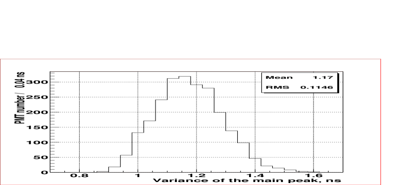
Figure 18: Statistics of the main peak width

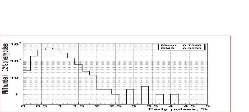
Figure 19: Statistics of the early pulses probability

And, finally, the amount of the late pulses, arriving with a delay greater than $3\sigma$ with respect to the main peak in the time spectrum, is the last characteristic of the time spectrum of PMT. The results are shown in Fig.20. The mean observed amount of late pulses is $7.9\%$ and corresponds to the CFD threshold set at the level of 0.17 p.e. The total probability to observe elastically scattered photoelectron, as follows from the analysis of the average transit time spectra, is $2.4\%$. This value is much closer to the one measured in ETL factory tests. The reasons for this discrepancy is the lower threshold in our measurements. The direct check with a CFD threshold set at the level of 0.3.-0.4 p.e. gives much lower values for the late pulses.

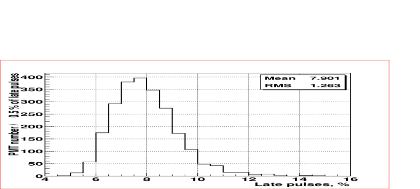
Figure 20: Statistics of the late pulses probability

5 Afterpulses

5.1 Afterpulses spectrum structure

A photoelectron striking a residual gas trapped in the photomultiplier can ionize a gas molecule, the ionized molecule will be accelerated back to the cathode releasing several photoelectrons, thus forming an undesirable satellite pulse [9]. The study of the ionic afterpulses was performed e.g. in [10]. In [11] afterpulse formation have been systematically studied directly introducing the trace amounts of various gases into photomultiplier tubes. A photomultiplier exhibit the phenomenon of afterpulses in the microsecond range with total afterpulses rate $p_{a}$ ranging from 0.1% to 5%. The upper limit usually is guaranteed by the manufacturer for the specified HV. It should be noted, that the origin of the afterpulses in PMTs is still being discussed.

The afterpulse rate $p_{a}$ is usually cited for the single photoelectron response and a certain time region after the main pulse. If a PMT is hit by a light pulse producing precisely n p.e. and the afterpulse production is independent for each initial electron, then the mean number of afterpulses will be defined by the following relation:

$$p_{a}(n)=n\cdot p_{a}$$ (10)

The value of $p_{a}(n)$ in (10) in principle can be greater than 1 for large $n$, but the value of $p_{a}$ can not exceed 1, otherwise the PMT will go into autogenerating regime.

For the series of the PMT responses to the light source with a mean intensity corresponding to $\mu$ p.e. with a Poisson law of the registered p.e. one should provide proper averaging over the Poisson probabilities of the registering precisely n p.e.:

$$p_{a}(\mu)=\frac{\sum P(n)p_{a}(n)}{1-P(0)}=\frac{\mu\cdot p_{a}}{1-e^{-\mu}}.$$ (11)

The delimiter in (11) reflects the fact that the afterpulses by their definition are following the main pulse. For the values $\mu\ll 1$ (11) will be reduced to:

$$p_{a}(\mu)\simeq p_{a}.$$ (12)

For flashes with a large number of initial photoelectrons secondary afterpulses are probable. The probability of observing secondary pulse is $p_{a}^{sec}=<N>\cdot p_{a}^{2}$, where $<N>$ is the mean number of secondary electrons produced in the afterpulses event

Formulae (10)-(11) are true as well for the afterpulses rate $p_{a}(\mu,t)\Delta t$ in the interval $\Delta t$ at any time $t$ under the same assumptions. The last formula is the basic in the practical afterpulses measurements. One can see that the afterpulse rate due to the low intensity light source coincide with the rate of the afterpulses of the single p.e. response.

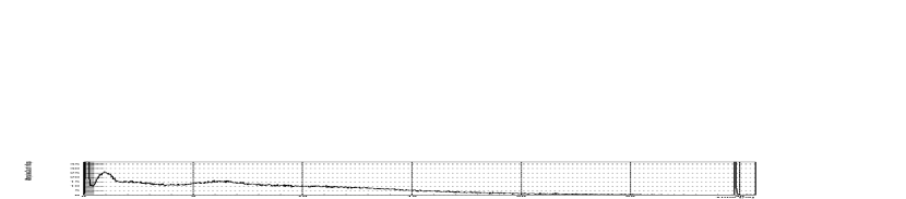
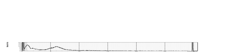
Figure 21: Measured afterpulse rate for 4 different PMTs.

The afterpulse probability for the more than 2000 ETL PMTs has been measured at the PMT test facility at the Gran Sasso Laboratory in the frame of the Borexino program. It should be noted that Multihit TDC was used in the measurements in contrast to the more common correlation measurements with ordinary start-stop TDC or multichannel analyzers. In such a way the acquired afterpulse spectra can in principle contain multiple afterpulses (up to 15; the system was adjusted to measure the time of arrival of the main pulse as the first one). The discriminator threshold was set approximately at the level of 0.2 p.e. and was checked out after the measurements. The mean measured threshold was $0.17$ p.e.

The afterpulse spectra for 4 different PMTs are presented in Fig.21. The afterpulse rates are presented in the figure as the excess dark rate counted in Kcps. The peak at $t\simeq 30$ $\mu$s is due to the next laser flash inside the MTDC gate (laser flashed at $\simeq 33$ kHz). The amount of pulses in this peak has been used to check the laser intensity.

The spectra in Fig.21 have common features: relatively narrow peaks about 1 $\mu s$ and 2 $\mu$s, wider peaks around 6.5 $\mu s$ and 12 $\mu s$ , and at $t>25$ $\mu s$ no afterpulses are present. The analysis performed for the set of 2300 PMTs showed no significant dependence of the afterpulses amount on the applied voltage. The difference in the position of the peaks at 6 $\mu$s for the PMT with working voltage 1200 V and 1800 V is only 150 ns. This feature allows to perform averaging of the afterpulse spectra over the set of all PMTs. The procedure of averaging is performed as follows:

1. Using the measured value of the dark rate, the contribution $N_{dark}$ of the random coincidences at one bin was calculated and extracted from the value at each bin.

2. For each histogram the position of the main peak in the distribution and its integral are found and the histogram is shifted in order to put its maximum at the position corresponding to $t=0$. The spectrum is normalized on the integral of the main peak (number of true triggers).

3. All the histograms are summed together and normalized on the integral of the main peak once more. The obtained histogram contains the mean characteristics of a sample of the PMTs used with a main peak at the position $t=0$.

The resulting histogram is presented in Fig.22. The weak peak at 5 $\mu$s appears at the histogram together with the already mentioned ones. The afterpulse amount is presented in the histogram as an excess rate in Kcps.

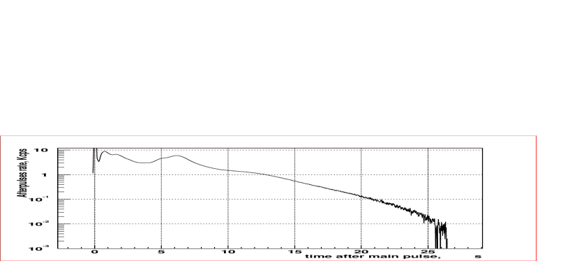
Figure 22: Average spectrum of afterpulses.

The systematic study of the origin of the afterpulses is now in progress and will be the subject of another article. Below we will give the main afterpulse characteristics.

5.2 Afterpulse characterization

For studying the afterpulses 3 regions of interest were chosen: $0.4-1.0$ $\mu$s, $1.0-3.6$ $\mu$s and $3.6-12.8$ $\mu$s. The amount of the afterpulses in these regions and the total amount of afterpulses are presented in Fig.23-26. The mean (total) count of afterpulses calculated from the Fig.22 is $4.9\%$ (see Fig.26 as well).

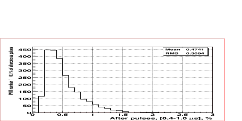
Figure 23: Afterpulses in the region $0.4-1.0$ $\mu$s,

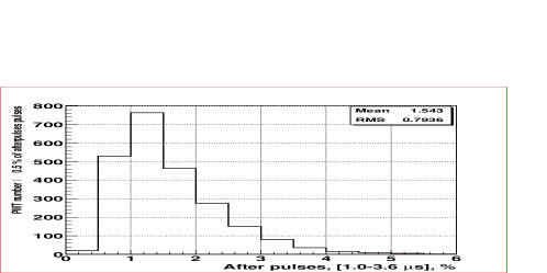
Figure 24: Afterpulses in the region $1.0-3.6$ $\mu$s,

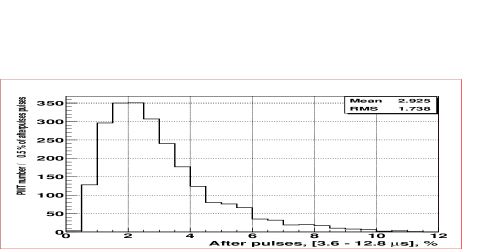
Figure 25: Afterpulses in the region $3.6-12.8$ $\mu$s,

Figure 26: Afterpulses in the region $0.4-12.8$ $\mu$s,

The mean excess rate of the afterpulses and the average peak positions in each of 3 regions is presented in Table 2. The total afterpulse rate measured in the test facility is somewhat greater than the one reported by the manufacturer. Indeed, we found a factor 2 discrepancy. The possible reason could be the different regime of the PMT operation, in our case the PMT are operating at a gain of $2\times 10^{7}$ in comparison with the gain of $1\times 10^{7}$ of the regime recommended by manufacturer. Another possible reason could be the different discriminator threshold setting. The measurements with a different threshold showed that the amount of afterpulses decreases with a higher threshold. In particular, with a threshold set at 0.4 p.e. level one obtains practically the same values as provided by ETL.

region ($\mu$s)	$0.4-1.0$	$1.0-3.6$	$3.6-12.8$	$12.8-25$
Total amount, %	0.5	1.5	2.9	0.1
average peak position, $\mu$s	0.88	1.74	6.38	not defined
standard deviation from	0.09	0.22	0.30
the average position, $\mu$s
mean excess rate in the peak, Kcps	21.7	16.7	15.4	3.8
standard deviation from the	13.6	7.9	7.8	2.7
mean excess rate, Kcps

Table 2: Main characteristics of the afterpulses.

6 Concluding remarks

More than 150 PMTs were rejected during the acceptance tests of 2350 PMTs delivered from the manufacturer. The main reasons were the high dark rate (58 PMTs) and the high afterpulse rate (58 PMTs). 23 PMTs had a bad single electron charge resolution and 13 PMTs had a bad time resolution. The data is summed in Table 3. The selected 2200 PMTs, that met the requirements of the Borexino detector, were equipped with light concentrators and $\mu$-metal screens and installed in the detector. At the moment of the article submission (June, 2004), all the PMTs are installed in the Borexino detector, the detector is sealed and ready to be filled with water.

		The reason of rejection
	total	high	high	low charge	low time
	rejected	dark rate	afterpulse rate	resolution	resolution
Total number	152	58	58	23	13
Percentage of the rejected	100	38	38	15	9
Percentage of the tested	6.8	2.6	2.6	1	0.6

Table 3: The results of the acceptance test

7 Acknowledgements

We are deeply grateful to G.Korga and L.Papp who took an active part in the test. We also thank the LNGS staff for the warm atmosphere and the good working conditions. The job of one of us (O.S.) was supported by the INFN sez. di Milano, and he is personally indebted to Prof. G.Bellini for the possibility to work at the LNGS laboratory. The authors appreciate the help of M.Laubenstein in preparation of the manuscript.

Credit is given to the developers of the CERN ROOT program [13], that was used in the calculations and to create all the figures of the article.

References

- [1] G. Alimonti et al., Astroparticle Physics 16 (2002) 205-234.
- [2] A.Brigatti, A. Ianni, P.Lombardi, G. Ranucci and O. Ju. Smirnov, arXiv:physics/0406106, submitted to NIM.
- [3] R. Dossi, A. Ianni, G. Ranucci, O. Ju. Smirnov, NIM A451 (2000) 623-637.
- [4] O. Ju. Smirnov, Instruments and Experimental Techniques, Vol.46 No 3 (2003) 327-344.
- [5] O. Ju. Smirnov, Instruments and Experimental Techniques, Vol.45 No 3 (2002) 363.
- [6] O.Ju. Smirnov, P. Lombardi, G. Ranucci, Instruments and Experimental Techniques, Vol.47 No 1 (2004) p.69-77; also in arXiv:physics/0403029.
- [7] B.H.Candy. Rev.Sci.Instrum. 56 (1984) 183.
- [8] J.B. Birks, The theory and practice of scintillation counting, 1. ed. - Oxford : Pergamon Pr., 1964.
- [9] P.B.Coates, J.Phys. D6 (1973) 153.
- [10] S.Torre, T.Antonioni, and P.Benetti, Rev.Sci.Instrum. 54(12), 1983, 1777.
- [11] G.A.Morton, H.M.Smith, and R.Wasserman, Trans IEEE Nucl.Sci. NS-14, (1), 443 (1967)
- [12] D.F.Bartlett, A.L.Duncan, and J.R.Elliott, Rev.Sci.Instrum. 52(2), 1981, 265.
- [13] ROOT home page, http://root.cern.ch/