Space-frequency model of amplified spontaneous emission and super-radiance in free electron laser operating in the linear and non-linear regimes

Abstract

A three-dimensional, space-frequency model for the excitation of electromagnetic radiation in a free-electron laser is presented. The approach is applied in a numerical particle code WB3D, simulating the interaction of a free-electron laser operating in the linear and non-linear regimes. Solution of the electromagnetic excitation equations in the frequency domain inherently takes into account dispersive effects arising from the cavity and the gain medium. Moreover, it facilitates the consideration of statistical features of the electron beam and the excited radiation, necessary for the study of spontaneous emission, synchrotron amplified spontaneous emission (SASE), super-radiance and noise.

We employ the code to study the statistical and spectral characteristics of the radiation generated in a pulsed beam free-electron laser operating in the millimeter wavelengths. The evolution of radiation spectrum, excited when a Gaussian shaped bunch with a random distribution of electrons is passing through the wiggler, was investigated. Numerical results of spontaneous emission power along the wiggler are compared to analytical predictions in the linear regime. In the first few periods, the power is excited from shot-noise in the low-gain regime. An exponential growth of SASE in the high-gain regime is inspected after passing a sufficient number of periods, until saturation occurs when arriving to the non-linear regime of the FEL operation.

1 Introduction

Electron devices such as microwave tubes and free-electron lasers (FELs) utilize distributed interaction between an electron beam and electromagnetic radiation. Random electron distribution in the $e$-beam causes fluctuations in current density, identified as shot noise in the beam current [1]-[4]. Electrons passing through a magnetic undulator emit a partially coherent radiation which is called undulator synchrotron radiation [5]. The electromagnetic fields excited by each electron add incoherently, resulting in spontaneous emission [6]-[13]. When the electron beam is modulated or pre-bunched, the fields excited by electrons become correlated, and coherent summation of radiation fields from individual particles occurs. If all electrons radiate in phase with each other, the generated radiation becomes coherent (super-radiant emission).

In high-gain FELs, utilizing sufficiently long undulators, the spontaneous emission radiation excited in the first part of the undulator is amplified along the reminder of the interaction region resulting in self-amplified spontaneous emission (SASE) [14]-[18]. Super-radiant emission emerges if the electrons are injected into the undulator in a single short bunch (shorter than the oscillation period of the emitted radiation) [19]-[25] or enter as a periodic train of bunches at the frequency of the emitted radiation [26]-[30].

Investigation of spontaneous and super-radiant emissions, as well as SASE, call for analytical and numerical models, that can describe non-stationary stochastic processes involved in the generation of incoherent or partially coherent radiation. In addition to the statistical features of the electron beam and radiation, the model should take into account dispersive effects evolving in the medium, in which the radiation is excited. The model presented in this paper, utilizes an expansion of the total electromagnetic field (radiation and space-charge waves) in terms of transverse eigenmodes of the medium, in which the field is excited and propagates [31, 32]. The interaction between the electron beam and the electromagnetic field is described by a set of coupled-mode excitation equations, that expresses the evolution of mode amplitudes in the frequency domain. The excitation equations are solved self-consistently with the equation of particles motion, which describes the electron beam dynamics.

2 Presentation of the electromagnetic field in the frequency domain

The electromagnetic field in the time domain is described by the space-time electric ${\bf E}({\bf r},t)$ and magnetic ${\bf H}({\bf r},t)$ signal vectors. ${\bf r}$ stands for the $(x,y,z)$ coordinates, where $(x,y)$ are the transverse coordinates and $z$ is the axis of propagation. The Fourier transform of the electric field is defined by:

$${\bf E}({\bf r},f)=\int_{-\infty}^{+\infty}{\bf E}({\bf r},t)\ e^{+j2\pi ft}\ df$$ (1)

where $f$ denotes the frequency. Similar expression is defined for the Fourier transform ${\bf H}({\bf r},f)$ of the magnetic field. Since the electromagnetic signal is real (i.e. ${\bf E}^{\ast}({\bf r},t)={\bf E}({\bf r},t)$), its Fourier transform satisfies ${\bf E}^{\ast}({\bf r},f)={\bf E}({\bf r},-f)$.

Analytic representation of the signal is given by the complex expression:

$$\widetilde{\bf E}({\bf r},t)\equiv{\bf E}({\bf r},t)-j\,\widehat{{\bf E}({\bf r},t)}$$ (2)

where

$$\widehat{{\bf E}({\bf r},t)}=\int_{-\infty}^{+\infty}\frac{{\bf E}({\bf r},t^{\prime})}{t-t^{\prime}}\ dt^{\prime}$$ (3)

is the Hilbert transform of ${\bf E}({\bf r},t)$. Fourier transformation of the analytic representaion (2) results in a ’phasor-like’ function $\widetilde{\bf E}({\bf r},f)$ defined in the positive frequency domain and related to the Fourier transform by:

$$\widetilde{\bf E}({\bf r},f)=2\,{\bf E}({\bf r},f)\cdot u(f)=\left\{\begin{array}[]{cl}2\,{\bf E}({\bf r},f)&f>0\\ 0&f<0\end{array}\right.$$ (4)

The Fourier transform can be decomposed in terms of the ’phasor like’ functions according to:

$${\bf E}({\bf r},f)=\frac{1}{2}\,\widetilde{\bf E}({\bf r},f)+\frac{1}{2}\,\widetilde{\bf E}^{\ast}({\bf r},-f)$$ (5)

and the inverse Fourier transform is then:

$${\bf E}({\bf r},t)=\int_{-\infty}^{+\infty}{\bf E}({\bf r},f)\ e^{-j2\pi ft}\ df=\Re\left\{\int_{0}^{\infty}\widetilde{\bf E}({\bf r},f)\ e^{-j2\pi ft}\ df\right\}$$ (6)

3 The Wiener-Khinchine and Parseval theorems for electromagnetic fields

The cross-correlation function of the time dependent electric ${\bf E}({\bf r},t)$ and magnetic ${\bf H}({\bf r},t)$ fields is given by:

$$R_{EH}(z,\tau)=\int_{-\infty}^{+\infty}\left\{\int\int\left[{\bf E}({\bf r},t+\tau)\times{\bf H}({\bf r},t)\right]\cdot\hat{\bf z}\ dx\,dy\right\}\ dt$$ (7)

Note that for finite energy signals, the total energy carried by the electromagnetic field is given by ${\mathcal{W}}(z)=R_{EH}(z,0)$

According to the Wiener-Khinchine theorem, the spectral density function of the electromagnetic signal energy $S_{EH}(z,f)$ is related to the Fourier transform of the cross-correlation function $R_{EH}(z,\tau)$ through the Fourier transformation:

$$\mbox{}S_{EH}(z,f) = \int_{-\infty}^{+\infty}R_{EH}(z,\tau)\ e^{+j2\pi f\tau}\ d\tau=\int\int\left[{\bf E}({\bf r},f)\times{\bf H}^{\ast}({\bf r},f)\right]\cdot\hat{\bf z}\ dx\,dy=$$ (10)

$$= \left\{\begin{array}[]{ll}\int\int\frac{1}{4}\left[\widetilde{\bf E}({\bf r},f)\times\widetilde{\bf H}^{\ast}({\bf r},f)\right]\cdot\hat{\bf z}\ dx\,dy&f>0\\ \int\int\frac{1}{4}\left[\widetilde{\bf E}({\bf r},-f)\times\widetilde{\bf H}^{\ast}({\bf r},-f)\right]^{\ast}\cdot\hat{\bf z}\ dx\,dy&f<0\end{array}\right.$$

Following Parseval theorem, the total energy carried by the electromagnetic field can also be calculated by integrating the spectral density $S_{EH}(z,f)$ over the entire frequency domain:

$${\mathcal{W}}(z) = \int_{-\infty}^{+\infty}S_{EH}(z,f)\ df=$$ (11)

$$= \int_{0}^{\infty}\left[\int\int\frac{1}{2}\ \Re\left\{\widetilde{\bf E}({\bf r},f)\times\widetilde{\bf H}^{\ast}({\bf r},f)\right\}\cdot\hat{\bf z}\ dx\,dy\right]\ df$$

We identify:

$$\frac{d{\mathcal{W}}(z)}{df}=\frac{1}{2}\ \Re\left\{\int\int\left[\widetilde{\bf E}({\bf r},f)\times\widetilde{\bf H}^{\ast}({\bf r},f)\right]\cdot\hat{\bf z}\ dx\,dy\right\}$$ (12)

as the spectral energy distribution of the electromagnetic field (over positive frequencies).

4 Modal presentation of electromagnetic field in the frequency domain

The ’phasor like’ quantities defined in (4) can be expanded in terms of transverse eigenmodes of the medium in which the field is excited and propagates [32]. The perpendicular component of the electric and magnetic fields are given in any cross-section as a linear superposition of a complete set of transverse eigenmodes:

$$\widetilde{\bf E}_{\perp}({\bf r,f}) = \sum_{q}\left[C_{+q}(z,f)\,e^{+jk_{zq}z}\ +\ C_{-q}(z,f)\,e^{-jk_{zq}z}\right]\,\widetilde{\bf{\mathcal{E}}}_{q\perp}(x,y)$$

$$\widetilde{\bf H}_{\perp}({\bf r,f}) = \sum_{q}\left[C_{+q}(z,f)\,e^{+jk_{zq}z}\ -\ C_{-q}(z,f)\,e^{-jk_{zq}z}\right]\,\widetilde{\bf{\mathcal{H}}}_{q\perp}(x,y)$$ (13)

$C_{+q}(z,f)$ and $C_{-q}(z,f)$ are scalar amplitudes of the $q$th forward and backward modes respectively with electric field $\widetilde{\bf{\mathcal{E}}}_{q\perp}(x,y)$ and magnetic field $\widetilde{\bf{\mathcal{H}}}_{q\perp}(x,y)$ profiles and axial wavenumber:

$$k_{zq}=\left\{\begin{array}[]{lll}j\sqrt{k^{2}_{\perp q}-k^{2}}&k<k_{\perp q}&\mbox{(cut-off modes)}\\ \sqrt{k^{2}-k^{2}_{\perp q}}&k>k_{\perp q}&\mbox{(propagating modes)}\end{array}\right.$$ (14)

Expressions for the longitudinal component of the electric and magnetic fields are obtained after substituting the modal representation (13) of the fields into Maxwell’s equations, where source of electric current density $\widetilde{\bf J}({\bf r},f)$ is introduced:

$$\mbox{}\widetilde{E}_{z}({\bf r},f)=\sum_{q}\left[C_{+q}(z,f)\,e^{+jk_{zq}z}-C_{-q}(z,f)\,e^{-jk_{zq}z}\right]\,\widetilde{\mathcal{E}}_{qz}(x,y)+\frac{1}{j2\pi f\epsilon_{0}}\widetilde{J}_{z}({\bf r},f)$$

$$\mbox{}\widetilde{H}_{z}({\bf r},f)=\sum_{q}\left[C_{+q}(z,f)\,e^{+jk_{zq}z}+C_{-q}(z,f)\,e^{-jk_{zq}z}\right]\,\widetilde{\mathcal{H}}_{qz}(x,y)$$ (15)

The evolution of the amplitudes of the excited modes is described by a set of coupled differential equations:

$$\frac{d}{dz}C_{\pm q}(z,f)=$$ (16)

$$= \mp\frac{1}{2{\mathcal{N}}_{q}}\ e^{\mp jk_{zq}z}\int\int\left[\left(\frac{Z_{q}}{Z_{q}^{\ast}}\right){\widetilde{\bf J}}_{\perp}({\bf r},f)\pm\hat{\bf z}\widetilde{J}_{z}({\bf r},f)\right]\cdot{\widetilde{\mathcal{E}}_{q}}^{\ast}(x,y)\ dx\,dy$$

The normalization of the field amplitudes of each mode is made via each mode’s complex Poynting vector power:

$${\mathcal{N}}_{q}=\int\int\left[\widetilde{\bf{\mathcal{E}}}_{q\perp}(x,y)\times\widetilde{\bf{\mathcal{H}}}_{q\perp}^{\ast}(x,y)\right]\cdot\hat{\bf z}\ dx\,dy$$ (17)

and the mode impedance is given by:

$$Z_{q}=\left\{\begin{array}[]{ll}\sqrt{\frac{\mu_{0}}{\epsilon_{0}}}\frac{k}{k_{zq}}=\frac{2\pi f\mu_{0}}{k_{zq}}&\mbox{for TE modes}\\ \sqrt{\frac{\mu_{0}}{\epsilon_{0}}}\frac{k_{zq}}{k}=\frac{k_{zq}}{2\pi f\epsilon_{0}}&\mbox{for TM modes}\end{array}\right.$$ (18)

Substituting the expansion (13) in (12) results in an expression for the spectral energy distribution of the electromagnetic field (over positive frequencies) as a sum of energy spectrum of the excited modes:

$$\frac{d{\mathcal{W}}(z)}{df} = \sum_{\stackrel{{\scriptstyle q}}{{Propagating}}}\frac{1}{2}\left[|C_{+q}(z,f)|^{2}-|C_{-q}(z,f)|^{2}\right]\Re\left\{{\mathcal{N}}_{q}\right\}+$$ (19)

$$\hskip 85.35826pt+\sum_{\stackrel{{\scriptstyle q}}{{Cut-off}}}\Im\left\{C_{+q}(z,f)C_{-q}^{\ast}(z,f)\right\}\Im\left\{{\mathcal{N}}_{q}\right\}$$

The power spectral density carried by the propagating mode $q$ during a temporal period $T$ is given by the ensemble average:

$$\frac{dP_{q}(z)}{df}=\frac{1}{T}\ \overline{\left|C_{q}(z,f)\right|^{2}}\ {\mathcal{P}}_{q}$$ (20)

where ${\mathcal{P}}_{q}=\frac{1}{2}\Re\left\{{\mathcal{N}}_{q}\right\}$.

5 The electron beam dynamics

The state of the particle $i$ is described by a six-components vector, which consists of the particle’s position coordinates ${\bf r}_{i}=(x_{i},y_{i},z_{i})$ and velocity vector ${\bf v}_{i}$. The velocity of each particle, in the presence of electric ${\bf E}({\bf r},t)$ and magnetic ${\bf B}({\bf r},t)=\mu_{0}{\bf H}({\bf r},t)$ fields, is found from the Lorentz force equation:

$$\frac{d{\bf v}_{i}}{dz}=\frac{1}{\gamma_{i}}\left\{-\,\frac{e}{m}\,\frac{1}{v_{z_{i}}}\left[{\bf E}({\bf r}_{i},t)+{\bf v}_{i}\times{\bf B}({\bf r}_{i},t)\right]-{\bf v}_{i}\,\frac{d\gamma_{i}}{dz}\right\}$$ (21)

where $e$ and $m$ are the electron charge and mass respectively. The fields represent the total (DC and AC) forces operating on the particle, and include also the self-field due to space-charge. The Lorentz relativistic factor $\gamma_{i}$ of each particle is found from the equation for kinetic energy:

$$\frac{d\gamma_{i}}{dz}=-\,\frac{e}{mc^{2}}\,\frac{1}{v_{z_{i}}}\ {\bf v}_{i}\cdot{\bf E}({\bf r}_{i},t)$$ (22)

where $c$ is the velocity of light.

The time it takes a particle to arrive at a position $z$, is a function of the time $t_{0i}$ when the particle entered at $z=0$, and its instantaneous longitudinal velocity $v_{zi}(z)$ along the path of motion:

$$t_{i}(z)=t_{0_{i}}+\int_{0}^{z}\frac{1}{v_{z_{i}}(z^{\prime})}\ dz^{\prime}$$ (23)

The current distribution is determined by the position and the velocity of the particles in the beam:

$${\bf J}({\bf r},t)=-q\sum\limits_{i=1}^{N}\left(\frac{{\bf v}_{i}}{v_{z_{i}}}\right)\,\delta(x-x_{i})\ \delta(y-y_{i})\,\delta\left[t-t_{i}(z)\right]$$ (24)

here $q=\frac{I_{0}T}{N}$ is the charge of each of the $N$ macro particles in the simulation ($I_{0}$ is the DC current of the e-beam pulse of temporal duration $T$). The ’phasor like’ current density is given by:

$${\widetilde{\bf J}}({\bf r},f) = 2\,u(f)\int\limits_{-\infty}\limits^{+\infty}{\bf J}({\bf r},t)\ e^{-j2\pi ft}\ dt=$$ (25)

$$= -2q\sum\limits_{i=1}^{N}\left(\frac{{\bf v}_{i}}{v_{z_{i}}}\right)\,\delta(x-x_{i})\,\delta(y-y_{i})\ e^{-j2\pi ft_{i}(z)}\ u(f)$$

6 Numerical results

The WB3D code was used to investigate the excitation of spontaneous emission in a millimeter wave free-electron maser (FEM), with operational parameters given in Table 1. The corresponding dispersion curves of the FEM are shown in Fig. 1. When the beam energy is set to 1.375 MeV, there are two separated intersection points between the beam and waveguide dispersion curves, corresponding to the “slow” ($v_{g_{1}}<v_{z_{0}}$) and “fast” ($v_{g_{2}}>v_{z_{0}}$) synchronism frequencies 29 GHz and 100 GHz, respectively. Lowering the beam energy to 1.066 MeV, results in a single intersection at 44 GHz ("grazing limit"), where the beam dispersion line is tangential to the waveguide dispersion curve ($v_{g}=v_{z_{0}}$).

The evolution of spontaneous emission power spectrum in the vicinity of the upper synchronism frequency 100 GHz is drawn in Fig. 2.a. The power growth along the wiggler as a function of the wiggling periods $N_{w}$ is described in Fig. 2.b. In the first few periods, the mutual interaction between the electromagnetic radiation and the electron beam is small and the power amplification is low. Within this stage, the spontaneous radiation power increases proportional to $N_{w}^{2}$. An exponential growth of SASE is inspected later after passing a sufficient number of periods, revealing that the interaction enters to the high gain regime, until saturation occurs when arriving to the non-linear regime of the FEL operation. Fig. 3 describes the power evolution in the case of grazing.

Acknowledgments

The research of the second author (Yu. L.) was supported in part by the Center of Scientific Absorption of the Ministry of Absorption, State of Israel.

Table 1: Operational parameters of millimeter wave free-electron maser.

Accelerator
Electron beam energy:	$E_{k}$=1$\div$3 MeV
Electron beam current:	$I_{0}$=1 A
Wiggler
Magnetic induction:	$B_{w}$=2000 G
Period:	$\lambda_{w}$=4.444 cm
Waveguide
Rectangular waveguide:	1.01 cm $\times$ 0.9005 cm
Mode:	$TE_{01}$

Figure 1: FEM dispersion curves.

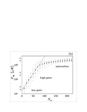
Figure 2: Evolution of spontaneous emission: (a) spectrum and (b) power along the wiggler. The beam energy is $E_{k}$=1.375 MeV.

Title Sheet

• Title of Paper: Space-frequency model of amplified spontaneous emission and super-radiance in free electron laser operating in the linear and non-linear regimes
  

• Author Name(s): Yosef Pinhasi, Yuri Lurie, Asher Yahalom, and
  Amir Abramovich
  

• Author Affiliation(s): The College of Judea and Samaria, Dept. of Electrical and Electronic Engineering — Faculty of Engineering, P.O. Box 3, Ariel 44837, Israel
  

• Requested Proceedings: Refereed

• Unique Session ID: Tu-O-05

• Classification Codes: 41.60.-m, 41.60.Cr, 52.75.Ms
  

• Keywords: free electron laser, spontaneous and super-radiant emission, SASE, space-frequency 3D model
  

• Corresponding Author Information:

  • Full Name: Yosef Pinhasi

  • Postal Address: The College of Judea and Samaria, Dept. of Electrical and Electronic Engineering — Faculty of Engineering, P.O. Box 3, Ariel 44837, Israel

  • Email Address: yosip@eng.tau.ac.il

  • Telephone: 972 - 3 - 9066 272

  • Fax: 972 - 3 - 9066 238

References

- [1] W. Schottky, Ann. Physik 57 (1918), 541
- [2] S. O. Rice, Bell System Tech. J. 23 (1944), 282
- [3] S. O. Rice, Bell System. Tech. J. 24 (1945), 46
- [4] L. D. Smulin and H. A. Haus, Noise in Electron Devices, (The Technology Press of Massachusetts Institute of Technology, 1959)
- [5] H. Motz, J. Applied Phys. 22 (1951), 527
- [6] B. Kincaid, J. Applied Phys. 48 (1977), 2684
- [7] J. M. J. Madey, Nuovo Cimento 50 B (1979), 64
- [8] A. N. Didenko et al., Sov. Phys. JTEP 49 (1979), 973
- [9] N. M. Kroll, Physics of quantum electronics: Free-electron generators of coherent radiation 7 (Addison-Wesley, Readings, Massachusettes, 1980)
- [10] K. J. Kim, AIP Conf. proceedings 184 (1989), 565
- [11] H. P. Freund et al., Phys. Rev. A 24 (1981), 1965
- [12] W. B. Colson, IEEE J. Quantum Electron. QE-17 (1981), 1417
- [13] H. A. Haus and M. N. Islam, J. Applied Phys. 54 (1983), 4784
- [14] R. Bonifacio, C. Pellegrini, L.M. Narducei, Optics Comm. 50 (1984), 373
- [15] K.J. Kim, Phys. Rev. Lett. 57 (1986), 1871
- [16] S. Krinsky, L.H. Yu, Phys. Rev. A 35 (1987), 3406
- [17] R. Bonifacio et al., Phys. Rev. Lett. 73 (1994), 70
- [18] E.L. Saldin, E.A. Schneidmiller, M.V. Yurkov, Optics Comm. 148 (1998), 383
- [19] R. Bonifacio, C. Maroli, and N. Piovella, Optics Comm. 68 (1988), 369
- [20] R. Bonifacio, B. W. J. McNeil, and P. Pierini, Phys. Rev. A 40 (1989), 4467
- [21] S. Cai, J. Cao, and A. Bhattachrjee Phys. Rev. A 42 (1990), 4120
- [22] N. S. Ginzburg and A. S. Sergeev, Optics Comm. 91 (1992), 140
- [23] F. Ciocci et al., Phys. Rev. Lett. 70 (1993), 928
- [24] A. Gover et al., Phys. Rev. Lett. 72 (1994), 1192
- [25] Y. Pinhasi and A. Gover, Nucl. Inst. and Meth. in Phys. Res. A 393 (1997), 393
- [26] M. P. Sirkis and P. D. Coleman, J. Applied Phys. 28 (1957), 527
- [27] R. M. Pantell, P. D. Coleman, and R. C. Becker, IRE Trans. Electron Devices ED-5 (1958), 167
- [28] I. Schnitzer and A. Gover, Nucl. Inst. and Meth. in Phys. Res. A 237 (1985), 124
- [29] A. Doria et al., IEEE J. Quantum Electron. QE-29 (1993), 1428
- [30] M. Arbel, A. Abramovich, A. L. Eichenbaum, A. Gover, H. Kleinman, Y. Pinhasi, Y. Yakover, Phys. Rev. Lett. 86, (2001), 2561
- [31] Y. Pinhasi, A. Gover, and V. Shterngartz, Phys. Rev. E 54 (1996), 6774
- [32] Y. Pinhasi, Yu. Lurie and Asher Yahalom, “Model and simulation of wide-band interaction in free-electron lasers”, accepted for publication in Nucl. Instr. and Meth. in Phys. Res. A (2001)