An automated and versatile ultra-low temperature SQUID magnetometer

Abstract

We present the design and construction of a SQUID-based magnetometer for operation down to temperatures $T\simeq 10$ mK, while retaining the compatibility with the sample holders typically used in commercial SQUID magnetometers. The system is based on a dc-SQUID coupled to a second-order gradiometer. The sample is placed inside the plastic mixing chamber of a dilution refrigerator and is thermalized directly by the ³He flow. The movement though the pickup coils is obtained by lifting the whole dilution refrigerator insert. A home-developed software provides full automation and an easy user interface.

I Introduction

The use of Superconducting QUantum Interference Devices (SQUIDs) gallopB in ultra-sensitive magnetic measurements systems may nowadays be considered as a standard technique, to the extent that several companies offer reliable and automated commercial SQUID magnetometers. However, no commercial magnetometer has yet become available for operation at millikelvin temperatures utilizing a dilution refrigerator. A few systems have been constructed that combine the sensitivity of SQUID magnetometery with the millikelvin temperature range attainable by means of ³He/⁴He dilution refrigerators paulsenB ; wernsdorfer00JAP(SQUID) ; bjornsson01RSI , at the cost of requiring the sample to be mounted on dedicated sample holders, which ensure the thermalization to the cold plate of the refrigerator by means of conducting thermal links.

We describe here a SQUID magnetometer designed to allow high-sensitivity measurements down to $T\sim 10$ mK, while retaining the compatibility with the sample holders used in commercial magnetometers. Moreover, we wanted to avoid building a system dedicated exclusively to SQUID magnetometery. Our setup can accommodate several different experimental probes, e.g. for nuclear magnetic resonance morello04CM , inductance-bridge-based ac-susceptometery morello03PRL and resistivity measurements. Finally, we wrote a software that fully automates the system and offers a very user-friendly interface to program the measurement sequences and analyze the data.

An example of research for which our setup was particularly designed is the field of metallic nanoclusters, which show spectacular quantum-size effects in their thermodynamic properties volokitin96N at very low temperatures, as a consequence of which their magnetic susceptibility is very small in this regime. Furthermore, since most of these materials are highly air-sensitive, it is a necessity to introduce and keep the sample in a sealed glass tube, that allows at the same time to perform preliminary measurements at $T>1.8$ K in commercial SQUID magnetometers and pre-check the quality of the sample in a fast and cheap way. The sample, in its sample holder, can thereupon be inserted in the ultra-low temperature SQUID magnetometer without need of any further manipulation, which constitutes an obvious advantage.

The really challenging part of the design consists in the fact that, like in most commercial and non-commercial nave80RSI ; genna91RSI magnetometers, to obtain the absolute value of the magnetization we need to move the sample through a gradiometer pick-up coil, but in our case the sample is at $T\geq 10$ mK inside the mixing chamber of the dilution refrigerator! The sample movement is needed because the coils of the gradiometer will never perfectly compensate one another, leaving an empty-coil signal that will add a spurious contribution to the measured magnetic moment, or even wash out the signal of the sample to be measured. As we shall discuss below, this has required a system that moves the whole dilution refrigerator insert.

II Dilution refrigerator

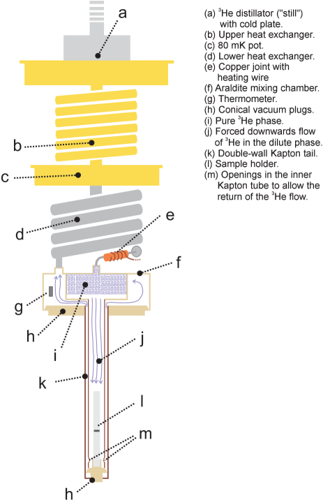
Figure 1: Scheme of the low-$T$ part of the dilution refrigerator. For clarity we omit the vacuum can and the radiation shields anchored at the still and at the 80 mK pot. Only the narrow tail of the refrigerator is inserted in the bore of a 9 T superconducting magnet (not shown).

Our ultra-low temperature setup is based on a Leiden Cryogenics MNK126-400ROF dilution refrigerator. Instead of the standard copper mixing chamber, we fitted the system with a specially designed plastic mixing chamber that allows the sample to be thermalized directly by the ³He flow. A scheme of the low-temperature part of the refrigerator is shown in Fig. 1. The mixing chamber consists of two concentric tubes, obtained by rolling a Kapton foil coated with Stycast 1266 epoxy. The tops of each tube are glued into concentric Araldite pots: the inner pot receives the downward flow of condensed ³He and, a few millimeters below the inlet, the phase separation between pure ³He phase and dilute ³He/⁴He phase takes place. The circulation of ³He is then forced downwards along the inner Kapton tube, which has openings on the bottom side to allow the return of the ³He stream through the thin space in between the tubes. Both the bottom of the Kapton tail and the outer pot are closed by conical Araldite plugs smeared with Apiezon N grease. The sample is typically placed inside a capsule filled with cotton and inserted in a plastic straw, fixed onto the bottom Aradite plug. Alternatively, for samples being air sensitive or having very small magnetic signal, one may largely reduce the background contribution of the holder by placing the sample between two Suprasil glass rods inside a Suprasil tube sinzigT , as shown in Fig. 2. In this way, the sample is placed in a symmetric configuration with respect to the pick-up coil systems, so that the only signal induced by the vertical movement is that originating from the sample space and the sample itself. Both types of sample holders are compatible with the commercial SQUID magnetometers (Cryogenic Consultant Limited S600c, Quantum Design MPMS-5 and MPMS-XL) available in our laboratory for magnetic measurements at $T>1.8$ K.

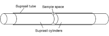
Figure 2: Sketch of the symmetric Suprasil glass sample holder.

The Kapton tail, which is about 35 cm long, is surrounded by two silver-plated brass radiation shields, one anchored at the 80 mK pot, the other at the still. The whole low-$T$ part of the refrigerator is closed by a vacuum can, which has itself a thin brass tail to surround the Kapton part of the mixing chamber, and is inserted into the bore of an Oxford Instruments 9 Tesla NbTi superconducting magnet. In this way, only Kapton and brass cylinders (plus the lowest Araldite plug) are placed in the high-field region, whereas all other highly-conducting metal parts (heat exchangers, 80 mK pot, ³He distillator, etc.) are outside the magnet bore and subject only to a small stray field. This design minimizes the eddy current heating resulting from moving the refrigerator through the pick-up coil of the SQUID magnetometer, while at the same time thermalizing the sample directly by the contact with the ³He flow. The excellent sample thermalization obtained is this way has already proven to be essential for NMR experiments on molecular magnets performed in the same refrigerator down to $T\simeq 15$ mK, whose success depends crucially on the efficient cooling of the nuclear spins morello04CM .

The temperature inside the mixing chamber is monitored by measuring, with a Picowatt AVS-47 bridge, the resistance of a Speer carbon thermometer placed in the outer part of the top Araldite pot. By adding an extra Speer thermometer (calibrated against the previous one) in the bottom of the Kapton tail, we have verified that the temperature is very uniform along the whole chamber (except in the presence of sudden heat pulses): even at the lowest $T$, the mismatch between the measured values is typically $\lesssim 0.5$ mK. During normal operation, the thermometer in the bottom of the tail is obviously omitted, to avoid its contribution to the measured magnetic signal. A Leiden Cryogenics Triple Current Source is used to apply heating currents to a manganin wire, anti-inductively wound and glued around a copper joint just above the ³He inlet in the mixing chamber. In this way we can heat the incoming ³He stream and uniformly increase the mixing chamber temperature.

For the ³He circulation we employ an oil-free pumping system, consisting of a Roots booster pump (Edwards EH500) with a pumping speed of 500 m³/h, backed by two 10 m³/h dry scroll pumps (Edwards XDS10) in parallel. The main pumping line is a $\varnothing$ 100 mm solid tube, fixed at the pump side with a flexible rubber joint that allows for an inclination of a few degrees, and is connected to the head of the fridge by a “T” piece with two extra rubber bellows, to reduce the vibrations transmitted by the pumping system. In this configuration, the system reaches a base temperature of 9 mK. The typical ³He circulation rate at the base temperature is $\dot{n}\sim 350$ $\mu$mol/s, and the cooling power at 100 mK is $\dot{Q}\sim 150$ $\mu$W. When the Kapton tail is replaced by a flat plug, $\dot{Q}$ can be increased up to 700 $\mu$W @ 100 mK and $\dot{n}\sim 1200$ $\mu$mol/s by applying extra heat to the still; with the tail in place it’s more difficult to increase the circulation rate, and $\dot{Q}$ @ 100 mK hardly exceeds 250 $\mu$W.

III Principles of SQUID magnetometery

A SQUID (Superconducting QUantum Interference Device) is basically an ultra-sensitive flux-to-voltage converter, that exploits the peculiar quantum properties of closed superconducting circuits. A detailed description of its working principle can be found in textbooks gallopB ; lounasmaaB , or in §2.4.1 of Ref. morelloT . Here we just recall that a dc-SQUID, like the one used in our system, consists of a superconducting ring interrupted by two Josephson junctions, $J_{1}$ and $J_{2}$, each characterized by a critical current $I_{c}$, which represents the maximum current that may flow through the junction without dissipation. The dc-SQUID is operated by biasing the junctions $J_{1}$ and $J_{2}$ with a current $I_{\mathrm{bias}}>I_{c}$, such that a voltage $V$ develops across them (Fig. 3). The essential feature is that the voltage can be modulated by an applied magnetic flux $\Phi$, since the critical current $I_{c}$ also depends on $\Phi$. One finds that the screening current $I_{s}$ that circulates in the SQUID ring is related to the critical current $I_{c}$ of the junctions (assumed to be identical) by:

$$I_{s}=\frac{I_{c}}{2}\left[\sin\varphi^{\prime}-\sin\left(\varphi^{\prime}-2\pi\frac{\Phi_{\mathrm{ext}}+LI_{s}}{\Phi_{0}}\right)\right],$$ (1)

where $\Phi_{0}=h/2e=2.07\times 10^{-15}$ Wb is the flux quantum, $L$ is the self-inductance of the ring and $\varphi^{\prime}$ is the shift in the phase of the superconducting order parameter which develops across each junction. $I_{c}$ is obtained by maximizing $I_{s}$, yielding the periodic form of $I_{c}(\Phi_{\mathrm{ext}})$ shown in Fig. 3. By properly choosing the bias conditions, the dc-SQUID operates therefore as a flux-to-voltage converter, where the external flux can be applied by injecting a current in the input coil. Notice that a small fraction of a flux quantum can produce voltage changes of the order of millivolts! In the practice a dc-SQUID is used in feedback mode by employing a so-called Flux-Lock Loop (FLL), i.e. adding a feedback coil that produces a compensating flux such that $V=const$. This increases the accuracy and the dynamic range of the measurement, and allows to implement noise-reducing detection schemes.

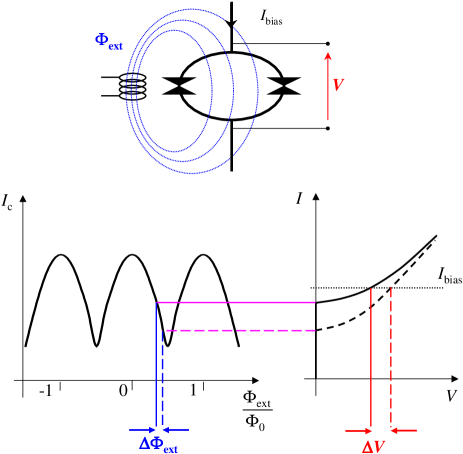
Figure 3: Working principle of a dc-SQUID as flux-to-voltage converter.

To use a dc-SQUID in an actual magnetometer, it is still necessary (except in a rather radical design like the “microSQUID” wernsdorfer00JAP(SQUID) ) to produce a current proportional to the magnetic moment of the sample to be measured. Such a current can be injected in the input coil to produce a flux that is coupled to the SQUID ring by the mutual inductance $\mathcal{M}$. Typically, the input current is obtained by constructing a closed superconducting circuit which includes the SQUID’s input coil on one side, and terminates with a pick-up coil on the other side. Once the circuit has been cooled down below the superconducting critical temperature, the enclosed flux is constant. Any change in the magnetic permeability of the circuit, for instance due to the sample, will result in a screening current that, while keeping the total flux constant, produces the required flux in the input coil. In our case, the change in permeability of the pick-up circuit is obtained by vertically moving the whole dilution refrigerator, whose tail, that contains the sample, is inserted in the pick-up coil.

Because of the high sensitivity, it is essential to make sure that no sources of flux other than the sample may couple with the SQUID. This can be done by employing a gradiometer, which in its simplest form consists of two coils wound in opposite direction, so that the flux produced by any uniform magnetic field cancels out, and only the gradient of $B$ can be detected (first-order gradiometer). A further improvement is the second-order gradiometer, shown in Fig. 4, which is obtained by inserting a coil with $2N$ windings between two coils with $N$ turns each, wound opposite to the central one. This design eliminates also the effects of linear field gradients. Furthermore, according to the reciprocity principle mallinson66JAP , the flux $\Phi$ produced in a coil of arbitrary geometry by a magnetic moment $\mu$ at position $\vec{r}$ is related to the field $\vec{B}(\vec{r})$ produced by the same coil in $\vec{r}$ when carrying a current $I$ such that:

$$\vec{B}\cdot\vec{\mu}=\Phi I.$$ (2)

The field produced by a single-loop coil is equivalent to the field of a magnetic dipole, whereas a first-order gradiometer is a magnetic quadrupole, and a second-order is an octupole, so that the fields they produce vary in space like $r^{-3}$, $r^{-4}$ and $r^{-5}$, respectively. From Eq.(2) it is clear that a second-order gradiometer is the least sensitive to magnetic fields produced outside of the coil system.

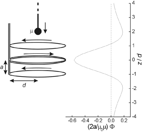
Figure 4: A second-order gradiometer in Helmoltz geometry ($a=2d$) and the magnetic flux induced by a dipole moving along $z$. Notice that the side peaks in $\Phi(z)$ do not coincide with the positions of the external coils. The factor $a$ in the $x$-axis scale is obtained by using the second form of Eq. (4).

The magnetic moment of the sample can be detected by moving it through the pick-up coil. The enclosed flux is easily obtained from the flux induced by a dipole with magnetic moment $\vec{\mu}\parallel\vec{z}$ at a position $z$ along the axis in a loop of radius $a$ placed at $z=z_{0}$:

$$\Phi_{\mathrm{loop}}(z)=\frac{\mu_{0}}{2}f(z-z_{0})\mu,$$ (3)

$$f(z-z_{0})=\frac{a^{2}}{[a^{2}+(z-z_{0})^{2}]^{3/2}}=$$

$$\frac{1}{a}\left[1+\frac{z_{0}^{2}}{a^{2}}\left(\frac{z}{z_{0}}-1\right)^{2}\right]^{-3/2}.$$ (4)

If the upper and lower coils of the gradiometer are placed at $z=d$ and $z=-d$, respectively, then the total picked-up flux is:

$$\Phi_{\mathrm{pu}}(z)=N\frac{\mu_{0}}{2}[f(z-d)-2f(z)+f(z+d)]\mu.$$ (5)

When adopting the Helmoltz geometry, $a=2d$, the resulting $\Phi(z)$ is shown in Fig. 4.

The picked-up flux is related to the screening current in the pickup circuit, $I_{S}$, by:

$$\Phi_{\mathrm{pu}}=(L_{\mathrm{pu}}+L_{\mathrm{leads}}+L_{\mathrm{in}})I_{S},$$ (6)

where $L_{\mathrm{pu}}$, $L_{\mathrm{leads}}$ and $L_{\mathrm{in}}$ are the inductances of the pick-up coil, the leads and the SQUID input coil, respectively. The flux at the SQUID sensor $\Phi_{\mathrm{SQUID}}$ is thus given by:

$$\Phi_{\mathrm{SQUID}}=\mathcal{M}I_{s}=f_{\mathrm{tr}}\Phi_{\mathrm{pu}},$$

$$f_{\mathrm{tr}}=\frac{\mathcal{M}}{L_{\mathrm{pu}}+L_{\mathrm{leads}}+L_{\mathrm{in}}},$$ (7)

where $f_{\mathrm{tr}}$ is the flux-transfer ratio claassen75JAP .

IV Design and construction of the pick-up circuit

The circuitry for our SQUID magnetometer is, with a few additions, based on the principles discussed above. The niobium dc-SQUID sensor is part of a Conductus LTS iMAG system, which includes a FLL circuitry to be placed just outside the cryostat, and is connected to the SQUID controller by a hybrid optical-electrical cable. To couple a magnetic signal to the SQUID we constructed a second-order gradiometer by winding a $\varnothing$ $100$ $\mu$m NbTi wire on a brass coil-holder, to be inserted in the bore of the Oxford Instruments 9 T NbTi superconducting magnet. The gradiometer coils have $\varnothing$ $36$ mm ($a=18$ mm) and $d=9$ mm. The choice of the diameter is constrained by the $\varnothing$ $34$ mm vacuum can of the refrigerator that contains the sample. The leads of the pick-up circuit, which are tightly twisted and shielded by a Nb capillary, are screwed onto the input pads of the SQUID to obtain a closed superconducting circuit. The input inductance of the SQUID sensor is $L_{\mathrm{in}}=600$ nH; since $L_{\mathrm{leads}}\sim 200$ nH and, given the dimensions, $L_{\mathrm{pu}}\sim L_{\mathrm{in}}+L_{\mathrm{leads}}$ already with $N=1$, it follows from Eq. (7) that the most convenient choice of windings for the gradiometer is 1-2-1 (recall that $\Phi_{\mathrm{pu}}\propto N$ but $L_{\mathrm{pu}}\propto N^{2}$). The mutual inductance between SQUID ring and input coil is $\mathcal{M}=10$ nH, which means that $f_{\mathrm{tr}}\sim 1/200$.

The FLL included in the Conductus electronics is able to compensate for $500$ $\Phi_{0}$ at the SQUID ring, which means that a maximum flux $\Phi_{\mathrm{pu}}^{\mathrm{(max)}}=500/f_{\mathrm{tr}}\sim 10^{5}$ $\Phi_{0}$ can be picked up by the gradiometer without saturating the system. The maximum measurable magnetic moment $\mu^{\mathrm{(max)}}$ is therefore [cf. Eq. (5) and Fig. 4]:

$$\mu^{\mathrm{(max)}}\approx\frac{2a}{0.6\mu_{0}}\Phi_{\mathrm{pu}}^{\mathrm{(max)}}\sim 10^{18}\mu_{B}\sim 10^{-5}\mathrm{\ Am^{2}}.$$ (8)

In order to extend the dynamic range, we have built an extra flux transformer on the pick-up circuit, which allows to introduce a magnetic flux from the outside to compensate for the flux induced by the sample. By using the SQUID as a null-meter, there is the extra advantage that no current circulates in the pick-up circuit, thus the field at the sample is precisely the field produced by the magnet, without the extra field that would be produced by a current in the gradiometer. The flux transformer consists of 16 turns of NbTi wire, wound on top of one loop of the pick-up wire and shielded by a closed lead box. In the same box we tightly glued the pick-up leads on top of a 100 $\Omega$ chip resistor, which is used to locally heat the circuit above the superconducting $T_{c}$ and eliminate the trapped flux. The flux transformer is fed by a Keithley 220 current source, whereas the heater is operated by one of the three current sources in the Leiden Cryogenics Triple Current Source used for the refrigerator. Both sources are controlled by the software described in Sect. VII.

Despite the efforts to isolate the system from external vibrations, the powerful pumps for the dilution refrigerator still provide a non-negligible mechanical noise. In particular, the Roots pump has a vibration spectrum with a lowest peak at $\sim 25$ Hz. To prevent the possible flux changes induced by such vibrations when coupled to a magnetic field, we added an extra low-pass filter on the pick-up circuitmeschkeT in the form of a 17 mm long $\varnothing$ $0.3$ mm copper wire in parallel with the pick-up leads. At $T=4.2$ K such a wire has a resistance $R\simeq 11$ $\mu\Omega$, which together with the input inductance $L_{\mathrm{in}}=600$ nH of the SQUID yields a cutoff frequency $f_{l.p.}=(1/2\pi)(R/L_{\mathrm{in}})\simeq 3$ Hz. The filter is contained in a separate Pb-shielded box inserted between the flux transformer and the SQUID. The pick-up leads and the copper wire are contacted via Nb pads.

A picture of the SQUID circuitry is shown in Fig. 5. The SQUID, the filter and the flux transformer are mounted on a radiation shield of the magnet hanging. The whole system is inserted in a 90 liter helium cryostat produced by Kadel Engineering. The magnet hanging is stabilized by triangular phosphor-bronze springs (not shown in Fig. 5) that press against the inner walls of the cryostat.

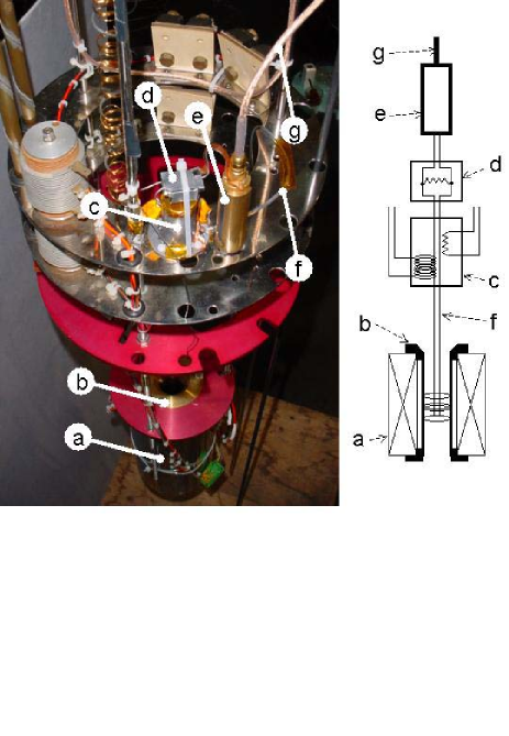
Figure 5: Picture and scheme of the SQUID circuitry. (a) Superconducting magnet. (b) Coil holder. (c) Flux transformer and heater in lead shield. (d) 3 Hz lead shielded low-pass filter. (e) SQUID sensor. (f) Pick-up leads with Nb capillary shield. (g) SQUID cryocable.

V Vertical movement

The movement of the sample through the gradiometer is obtained by lifting the whole dilution refrigerator. For this purpose, the refrigerator is fixed on a movable flange, while the top of the cryostat is closed by a rubber bellow. On the flange we screwed the nuts of three recirculating balls screws (SKF SN3 $20\times 5\mathrm{R}$), which allow a very smooth displacement of the nut by turning the screw. The base of each screw is mounted on ball bearings and is fitted with a gearwheel. The gearwheels are connected by a toothed belt (Brecoflex 16 T5 / 1400) driven by a three-phase AC servomotor (SEW DFY71S B TH 2.5 Nm) that can exert a torque up to 2.5 Nm. In this way, the rotation of the servomotor is converted into the vertical movement of the dilution refrigerator insert. The movement is so smooth that the consequent vibrations are hardly perceptible and do not exceed the vibrations due to the ³He pumping system.

The motor is driven by a servo-regulator (SEW MDS60A0015-503-4-00) that can be controlled by a computer. For safety reasons an electromagnetic brake is fitted, that blocks the motor in case of power failure. In addition, a set of switches is mounted along one of the pillars that support the screws: when the flange reaches the highest or the lowest allowed position, the switches force the motor to brake, independently of the software instructions. The maximum allowed vertical displacement is 10 cm.

A picture of the top of the cryostat with the vertical movement elements is shown in Fig. 6.

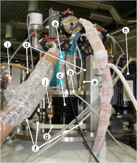
Figure 6: Picture of the top of the cryostat, with the elements for the vertical movement. (a) Head of the dilution refrigerator. (b) Movable flange. (c) Rubber bellow. (d) Screws. (e) Nut with recirculating balls. (f) Gearwheels. (g) Belt. (h) Servomotor. (i) SQUID FLL electronics. (j) Feedthrough to the SQUID cryocable.

VI Grounding and shielding

The shielding of the SQUID sensor and electronics is of course a crucial issue for the successful design of a SQUID-based magnetometer. As mentioned in §IV, the low-temperature parts are shielded by superconducting Pb boxes or Nb capillaries. As for the electronics outside the cryostat, the Conductus iMAG system provides hybrid optical-electrical cables for the communication between the SQUID controller and the FLL electronics on top of the cryostat, but in the cable that connects the FLL to the SQUID sensor, the ground is used as return line for the signals. This means that any ground loop involving the SQUID electronics will completely destroy the functionality of the system. Obviously, all the outer metallic parts in the system (e.g. the case of the SQUID sensor, the vacuum feedthrough for the cryocable, etc.) are connected to the same electrical ground, including the GPIB communication terminals.

The best way to avoid ground loops in the SQUID system would be to ground the SQUID sensor and its cable at the cryostat (and take care that it remains a very clean ground), and connect the controller to an isolation transformer vleemingT . This method is not practicable when communication with the computer via the GPIB bus is needed, and the same computer is connected to another instrument that requires a common ground with the cryostat (this is the case for the Picowatt AVS-47 resistance bridge). The only choice is therefore to ground the controller at its power cord and float the whole SQUID circuitry, all the way to the SQUID sensor inside the cryostat and the shields of the pick-up circuit (which must be connected to the SQUID ground). This is already a rather cumbersome operation, but it’s not yet sufficient. We found out that, in this configuration, the FLL electronics and the room-temperature cables around it are not enough shielded from the electromagnetic interference generated by the motor during the vertical movement of the dilution refrigerator (we obviously took care that the motor does not touch the cryostat ground). This sort of interference does not annihilate the functionality of the SQUID like a ground loop would do, nor does it simply induce an increase of the instrumental noise: the effect of bad shielding is that the SQUID system behaves as if it were connected to a non-superconducting, inductive circuit. This fault is hard to discover, since the inductive behavior of the pick-up system is one of the most expectable failures, which can be due to any weakening of the superconductivity in the circuit, for instance because of a bad contact on the SQUID input pads. The full functionality of the magnetometer was reached by enclosing the FLL and the room-temperature SQUID cables into an extra copper shield, grounded at the cryostat but separated from the SQUID ground.

VII Automation

The automation of the measurement system is achieved by connecting to a PC the iMAG SQUID controller, the Keithley 220 current course, the LC Triple Current Source, the Picowatt AVS 47 resistance bridge, and the SEW servo-regulator. The PC runs a home-written software, which provides an application with a single but flexible Graphical User Interface (GUI), containing all the required functionality: setup management, monitoring, measurement, automated sequence execution and data analysis. The application is written in Borland Delphi because of its power, ease of use, good documentation and rapid GUI development possibilities. The Windows user interface is primarily inspired upon the Quantum Design’s MultiVU application, included with their commercial Magnetic Property Measurement System (MPMS). This has the advantage of offering an interface that looks familiar to many users. The GUI consists of a Multiple Document Interface (MDI) with among other things a menu, a toolbar, a status bar, and removable panels. The MDI workspace is where the actual work is done in several subwindows, as shown in Fig. 7.

A set of tools are available for e.g. positioning the sample, setting a magnetic field, monitoring the temperature and performing “zero field oscillations”, i.e. oscillations of the applied field which are used to reduce the trapped flux in the magnet coil.

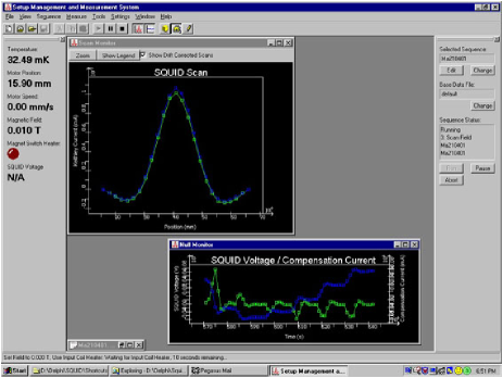
Figure 7: A screenshot of the application’s user interface. Information about temperature, vertical position, applied magnetic field, SQUID voltage and status of the program is constantly provided in the workspace. Additional windows are open, in this case, to monitor the result of the measurement and the nulling of the SQUID voltage.

In order to measure the magnetic moment of a sample, the response of the SQUID is measured while vertically moving the sample (i.e. the whole dilution refrigerator insert) along the gradiometer, as illustrated in Fig. 4. The sample can be positioned in two ways, using the so-called continuous or hold mode. In the continuous mode, the sample is positioned at the start of the trajectory and then set into a continuous motion. During the movement, readings are made at fixed time intervals. When the sample reaches the end of the trajectory, the movement is stopped. In the hold mode, the sample is moved for a short interval of time after which the motor is stopped and the SQUID reading is done, repeating this sequence until the final position is reached.

A reading can be done in direct or null mode. In the direct mode, one reads directly the SQUID voltage, which is proportional to the screening current that circulates in the pickup system. In null mode, the compensation current in the flux transformer is continuously being regulated by the software, using a proportional feedback controller which runs in the background, until the SQUID voltage is zero. A reading in null mode consists therefore of the current necessary to null the SQUID voltage. At the start of each measurement (“scan”), the sample is first accurately positioned at the starting point and then, if used, the nulling process is started. The measurement will then start and continue until the end point is reached. Typically two scans are done, an upward and a downward scan; the results of the two scans are corrected for the drift of the SQUID voltage, averaged and fitted to obtain the dipole moment.

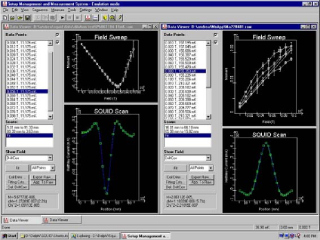
Figure 8: A screenshot of the data viewer. On the left-hand side we analyzed the field dependence of the magnetization of a Pb sample between 0 and 80 mT at $T=11$ mK. On the right-hand side, a sequence of magnetization curves of MnApy (see text) between 0 and 100 mT at four different temperatures.

Measurements can be managed, viewed and fitted using the built-in data viewer: an example is shown in Fig. 8. The data viewer consists of a set of controls and two graphs, one containing the fitted dipole moment of multiple scans and the other containing the single fitted scans.

In the end, the fitted dipole moment obtained from a set of scans which have been interpolated, averaged and fitted, represents one data point at a certain temperature and applied magnetic field. In general, we are interested in measuring the sample magnetization at several values of temperature and/or field. To do this automatically, an elementary scripting language has been implemented very similar to the way done in the MPMS MultiVU application. There are commands for, among other things, changing the sample position, setting a temperature, setting a field, heating and retuning the SQUID sensor, performing zero field oscillations and running a subsequence. All these commands can be nested in for-loop structures for measuring as a function of temperature or field. The sequence files are edited using a built-in sequence editor which supports the most common editing functions such as cut, copy, paste and undo. When a sequence is run, it can be paused, resumed, aborted and the execution status can be monitored.

As for the implementation, the application consists of a main core structure and modular components called “applets”. The core structure implements routines for the starting and stopping of the program, user interface, device initialization and communication, and the necessary menu items, tool buttons and shortcuts for starting the various components of the application. The applets are started from the main program and do all the work involving device communication, e.g. provide a tool for magnet management, monitor the status of the setup, null the SQUID using the FLL, do a set of scans, or execute a sequence. The applets which communicate with devices run in separate parallel threads to ensure communication without sacrificing performance of the main program. There are, for example, typically four threads running during a null-mode measurement:

• The main GUI thread

• A thread which monitors and displays the mixing chamber temperature, vertical sample position, magnet status and SQUID voltage. This thread communicates with devices not used by other applets.

• The measurement thread, which communicates with the servo regulator and the SQUID (in direct mode)

• The nuller thread which communicates with the SQUID and Keithley 220 current source

When an applet obtains information from a device, e.g. servomotor position, magnetic field or SQUID voltage, this information is shared with the other applets so that all applets stay informed about the global status of the system.

The applets communicate with the devices through a central abstract layer which encapsulates the device specific hardware communication and protocols. This central layer also makes it possible to start and stop the devices while the application is running. All the device’s functionality can additionally be simulated, which was very useful during the implementation phase: most of the application was written without using the experimental setup.

VIII Performance

In order to check the performance of our instrument, we first measured the magnetization of a small lead grain in a Quantum Design MPMS-XL magnetomter, then we mounted the sample, with the same sample holder, inside the mixing chamber of the dilution refrigerator. The results are shown in Fig. 9: at $T=4.5$ K, the data in our setup and in the MPMS-XL can be accurately superimposed, provided the correct calibration factor is chosen. By cooling down to $T=11$ mK, we still find the same slope of $M(H)$ and an expectedly higher critical field.

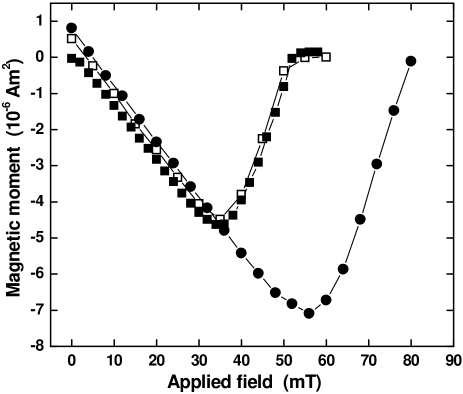
Figure 9: The magnetic moment of a small Pb grain, as measured in our setup (full symbols) and in a Quantum Design MPMS-XL magnetometer (open symbols). Squares: $T=4.5$ K, circles: $T=11$ mK.

As an example of dc-susceptibility experiment, we show in Fig. 10 a dataset obtained by measuring 1.9 mg of the paramagnetic salt manganese antipyrine Mn(C₁₁H₁₂ON₂)₆(ClO₄)₂ (MnApy), in a constant applied field $\mu_{0}H_{\mathrm{a}}=2$ mT while slowly cooling down the refrigerator. The paramagnetic centers in MnApy are the Mn²⁺ ions, with spin $S=5/2$ and gyromagnetic factor $g=2.00$. In this sort of measurements we typically use the “continuous + direct” mode, which allows to perform the scans rather quickly ($\sim 1$ min) as compared to the timescale of the temperature changes. The volume susceptibility $\chi=M/H=\mu\rho/(mH)$ ($m$ is the mass of the sample and $\rho=1.361\times 10^{3}$ kg/m³ is the density) can be obtained from the measured magnetic moment $\mu$ and compared with the expected behavior of a Curie paramagnet $\chi=C/T$, where $C=\mu_{0}\mathcal{N}g^{2}\mu_{B}^{2}S(S+1)/(3k_{B})$ is the Curie constant and $\mathcal{N}=5.927\times 10^{26}$ m^-3 is the number of spins per unit volume. In view of the high value of $\chi$ obtained at very low temperature, the comparison is meaningful only after having corrected the raw data for demagnetizing effects:

$$\chi_{\mathrm{corr}}=\frac{\chi_{\mathrm{raw}}}{1-D\chi_{\mathrm{raw}}},$$ (9)

where $D$ is the demagnetizing factor.

Since the sample is in powder form, $D$ will be an effective demagnetizing factor appropriate for the container (in this case a cylindrical capsule) filled with the grains. This is a notoriously complex problem that can only be solved in an approximate way. In a first step the relation should be found between the applied field $H_{\mathrm{a}}$ and the local field $H_{\mathrm{cont}}$ acting on a grain in the container. The dipolar contributions from the other grains can be divided in a shape-dependent part given by the demagnetizing factor $D_{\mathrm{cont}}$ of the container, and a “structural” part given by the packing of the grains. In a second step the relation between $H_{\mathrm{cont}}$ and the local field $H_{\mathrm{loc}}$ inside a grain should be found. The difference between $H_{\mathrm{cont}}$ and $H_{\mathrm{loc}}$ will now be due to the shape-dependent contribution related to the demagnetizing factor $D_{\mathrm{grain}}$ of the grain and the structural part arising from the crystal structure of the material.

In view of all the uncertainties involved, the simplest solution for the present purpose appears to assume all grains to have identical shape and to adopt, for both steps, the Lorentz approximation to estimate the contributions depending on the structural aspects. Thereby we shall also neglect the contributions from the dipoles inside the spheres. One then obtains:

$$D=D_{\mathrm{grain}}-\frac{1}{3}+f\left(D_{\mathrm{cont}}-\frac{1}{3}\right)=f\left(D_{\mathrm{cont}}-\frac{1}{3}\right),$$ (10)

where $f$ is the filling fraction (volume) of the container and where the last equality follows from the assumption $D_{\mathrm{grain}}=1/3$, i.e. we assume all grains to have a spherical shape. Given the shape of the sample holder, we estimate the demagnetizing factor of the container $D_{\mathrm{cont}}\simeq 0.7$, which yields $D\simeq 0.37f$. Taking for the filling factor $f\simeq 0.5$ (ideally packed spheres would yield $f\simeq 0.64$), we obtain the corrected volume susceptibility shown in Fig. 10. $\chi_{\mathrm{corr}}$ closely follows the calculated ideal Curie law, except for some small deviations below $\sim 0.2$ K. Such deviations are better appreciated when plotting $1/\chi_{\mathrm{corr}}$ vs $T$, as shown in the inset of Fig. 10. As it appears, the susceptibility remains always slightly lower than the value for an ideal Curie paramagnet. This can be attributed to a small crystal field anisotropy of the Mn²⁺ electron spins, which causes a reduction of the effective Curie constant at very low temperatures due to the depopulation of the excited energy levels in the zero-field split manifold algra77PhyB . Another reason for the deviation may be an (antiferromagnetic) ordering of the moments, e.g. due to the dipolar interactions between them. As an estimate of the interaction energy, $U$, we may consider the dipolar coupling between two Mn²⁺ spins $5/2$ at a distance $r\simeq 1$ nm in the MnApy compound. One then obtains $U=(\mu_{0}/4\pi)(g\mu_{B}S)^{2}/(k_{B}r^{3})\simeq 15$ mK. Although this estimate is very rough, it is an indication that such an ordering phenomenon may not be excluded.

The uncertainty in the choice of $D$ makes it rather delicate to analyze the data in more detail, but for the purpose of the present discussion we may state that the thermalization of the sample does not pose any special problem down to our lowest achievable temperature.

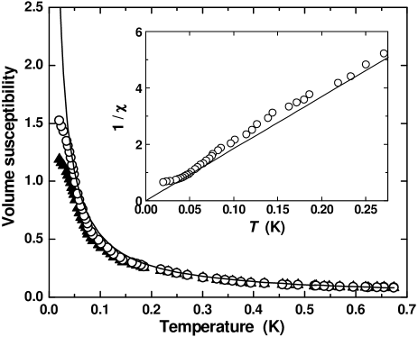
Figure 10: Full triangles: measured dc-susceptibility of MnApy in an applied field $\mu_{0}H_{\mathrm{a}}=2$ mT. Open circles: data corrected for the demagnetizing factor (see text). Solid line: calculated susceptibility according to the Curie’s law. Inset: inverse of the corrected susceptibility (open circles), fitted by the Curie-Weiss law (solid line), yielding $\Theta\simeq 14$ mK.

The typical noise at the SQUID in normal operation, i.e. while all the pumps are running and the dilution refrigerator insert is being moved, is $\sim 1$ mV, which translates into an equivalent magnetic noise $\sim 10^{-9}$ Am² ($10^{-6}$ emu). Measuring a magnetic moment $\sim 10^{-4}$ Am² (0.1 emu) in “null mode” requires a compensation current $\sim 30$ mA, which poses no problems to the compensation circuitry; this means that our system can easily cover a dynamic range of five orders of magnitude in magnetic moment.

As for the maximum applicable magnetic field, although the magnet itself can produce 9 T, the SQUID circuitry tends to become unstable above $\sim 0.2$ T. This a rather typical value when no special cautions are taken to stabilize the field and screen the SQUID circuitry from the stray fields: in specialized systemsgenna91RSI ; paulsenB , operation up to 8 T has been achieved by designing a dedicated magnet with large bore and by adding a NbTi superconducting shield around the sample- and pickup coils- space. We recall that our system is not dedicated uniquely to SQUID magnetometery and can accommodate, for instance, NMR experiments where the possibility of producing continuous field sweeps is essential.

^∗ Corresponding author:

L.J. de Jongh, e-mail: dejongh@phys.leidenuniv.nl

References

- (1) J. C. Gallop, SQUIDs, the Josepshon Effects and Superconducting Electronics, IOP publishing (Bristol, 1991).
- (2) C. Paulsen, chapter in Introduction to Physical Techniques in Molecular Magnetism: Structural and Macroscopic Techniques, Servicio de Publicaciones de la Universidad de Zaragoza (Zaragoza, 2001).
- (3) W. Wernsdorfer, D. Mailly, and A. Benoit, J. Appl. Phys. 87, 5094 (2000).
- (4) P. G. Björnsson, B. W. Gardner, J. R. Kirtley, and K. A. Moler, Rev. Sci. Instr. 72, 4153 (2001).
- (5) A. Morello, O. N. Bakharev, H. B. Brom, R. Sessoli, arXiv:cond-mat/0403107 (2004).
- (6) A. Morello, F. L. Mettes, F. Luis, J. F. Fernández, J. Krzystek, G. Aromí, G. Christou, and L. J. de Jongh, Phys. Rev. Lett. 90, 017206 (2003).
- (7) Y. E. Volokitin, J. Sinzig, L. J. de Jongh, G. Schmid, M. N. Vargaftik, and I. I. Moiseev, Nature 384, 621 (1996).
- (8) S. E. Nave and P. G. Huray, Rev. Sci. Instr. 51, 591 (1980).
- (9) J. C. Genna, S. Biston, J. C. Cotillard, P. Lethuillier, C. Faurin, P. Hostachy, R. Rocca-Valero, and J. Rouiller, Rev. Sci. Instr. 62, 1824 (1991).
- (10) J. Sinzig, Magnetism of Nanometer-Sized Particles, Ph.D. thesis, Leiden University (April 1997).
- (11) O. V. Lounasmaa, Experimental Principles and Methods Below 1 K, Academic Press (London, 1974).
- (12) A. Morello, Quantum Spin Dynamics in Single-Molecule Magnets, Ph.D. Thesis, Leiden University (March 2004); arXiv:cond-mat/0404049.
- (13) J. Mallinson, J. Appl. Phys. 37, 2514 (1966).
- (14) J. H. Claassen, J. Appl. Phys. 46, 2268 (1975).
- (15) M. Meschke, Untersuchung der magnetischen Eigenschaften kubischer Antiferromagnete, Ph.D. thesis, Technical University Berlin (January 2001).
- (16) B. J. Vleeming, The Four-Terminal SQUID, Ph.D. thesis, Leiden University (March 1998).
- (17) H. A. Algra, L. J. de Jongh, and R. L. Carlin, Physica 92B, 258 (1977).