Electrodynamics of a Magnet Moving through a Conducting Pipe

Abstract

The popular demonstration involving a permanent magnet falling through a conducting pipe is treated as an axially symmetric boundary value problem. Specifically, Maxwell’s equations are solved for an axially symmetric magnet moving coaxially inside an infinitely long, conducting cylindrical shell of arbitrary thickness at nonrelativistic speeds. Analytic solutions for the fields are developed and used to derive the resulting drag force acting on the magnet in integral form. This treatment represents a significant improvement over existing models which idealize the problem as a point dipole moving slowly inside a pipe of negligible thickness. It also provides a rigorous study of eddy currents under a broad range of conditions, and can be used for precision magnetic braking applications. The case of a uniformly magnetized cylindrical magnet is considered in detail, and a comprehensive analytical and numerical study of the properties of the drag force is presented for this geometry. Various limiting cases of interest involving the shape and speed of the magnet and the full range of conductivity and magnetic behavior of the pipe material are investigated and corresponding asymptotic formulas are developed.

I Introduction

I.1 Background and Significance

This work is based on the popular experiment which demonstrates magnetic damping by means of a permanent magnet falling through a conducting pipe clack ; saslow ; mac ; hahn . Such an arrangement has long been a favorite for demonstrating such topics as Faraday’s law of induction, Lenz’s law, eddy currents, inductive heating and magnetic damping. The underlying physical process is induction heating: the moving magnet creates a changing magnetic flux in its vicinity which induces circulating eddy currents within the pipe wall, thereby causing ohmic dissipation and generating a drag force on the magnet by virtue of energy conservation. The force itself is of course manifested as the action of the magnetic field generated by the eddies on the permanent magnet, with its retarding nature understood as a manifestation of Lenz’s law. A particularly vivid picture of this mechanism emerges if one views the magnet as an assembly of circulating atomic currents moving through the pipe. Lenz’s law then implies that the induced eddies in the pipe wall counter-circulate ahead of the moving magnet and co-circulate behind it. But this implies that the moving magnet is repelled in front and attracted in rear, hence acted upon by a retarding force.

The main contribution to the literature on this subject is Saslow’s paper saslow in which he treated the problem of eddy currents in thin conducting sheets quite generally, and as an example provided an approximate calculation of the drag force on a magnet falling inside a conducting pipe. MacLatchy et al. mac used other methods to derive Saslow’s result for the terminal speed and pointed out a sizable discrepancy between the predictions of this result and their measured values. These authors introduced a numerical modeling of the magnet which significantly improved the agreement. Following Saslow’s calculation saslow , analytical treatments of the magnet-pipe problem have considered the magnet as a point dipole moving at low speeds and the pipe as infinitely thin-walled and long. These assumptions imply that the only significant length parameter in the problem is the interior diameter of the pipe, and lead to a simple expression for the drag force. We will refer to this limit as the idealized model and derive it as a limiting case of our general solution in appendix B. The main sources of inaccuracy in this model are the point-dipole and thin-wall assumptions, with the low-speed approximation a potential source of inaccuracy as well.

I.2 Objectives and Limitations

Our objective in this work is to develop a rigorous formulation of the magnet-pipe system that avoids the approximations of the idealized model. To that end, we treat the case of an axially symmetric permanent magnet moving coaxially inside an infinitely long, conducting cylindrical shell of arbitrary thickness. By an axially symmetric magnet we mean a permanent magnet whose magnetization vector has an axially (or azimuthally) symmetric magnitude and a uniform direction parallel to the symmetry axis. Since any practical realization of this model will likely involve magnet speeds far smaller than the speed of light, we will restrict our treatment to nonrelativistic speeds, $v/c\ll 1$, where $v$ is the magnet speed and $c$ is the speed of light. On the other hand, we are including the possibility of the magnet being projected into the pipe thus allowing much higher speeds than can be attained by a magnet that starts to fall from rest under gravity. The restriction to nonrelativistic speeds implies that we are dealing with quasi-static sources and fields where displacement currents can be neglected jackson . This is so not only in the interior of the pipe where the inclusion of the displacement currents would amount to a minute correction of the order of ${(v/c)}^{2}$, but also within the pipe wall where conduction currents dominate displacement currents. To provide a basis for the latter assertion, we note that the basic time scale generated by the motion of the magnet is of the order of $R_{1}/v$, where $R_{1}$ is the inner radius of the pipe. This time scale corresponds to a frequency of the order of $v/R_{1}$, which implies that the ratio of displacement to conduction currents is of the order of ${\epsilon}_{0}v/\sigma R_{1}$ where $\sigma$ is the conductivity of the pipe wall si . For common metals and with $1\leq R_{1}\leq 10$ cm, this ratio is in the $3({10}^{-7}-{10}^{-10})v/c$ range. Since $v/c\ll 1$ by assumption, the ratio in question is seen to be vanishingly small.

The assumption of an infinitely long pipe is unavoidable if a manageable solution is desired. The error resulting from this assumption, on the other hand, is small if the magnet is not close to the pipe ends. To provide a basis for this assertion, one can use the idealized solution, appendix B, to estimate the dissipated power within the pipe segment that extends from its actual end to its idealized end (which is infinitely far). The ratio of this quantity to the total dissipated power is then an estimate of the leading finite-length correction to the drag force. This ratio is found to be of the order of ${({R}_{1}/D)}^{7}$, where $D$ is the distance from the magnet to the near end of the pipe and $R_{1}$ is the pipe’s interior diameter. For $R_{1}/D\lesssim 1/4$, for example, the expected correction would be of order ${10}^{-4}$ which is quite small as claimed. Similarly, the quasi-static approximation implies that the radiated power from the magnet-pipe assembly is negligible. To get an idea of the magnitude of such radiation, consider a permanent magnet with a magnetic dipole moment $\mathbf{m}$ moving longitudinally (i.e., parallel to $\mathbf{m}$) through free space at nonrelativistic speeds. The radiated power from such a source can be calculated and is found to be ${\mu}_{0}{m}^{2}{\ddot{v}}^{2}/30\pi{c}^{5}$ where ${\dot{v}}$ and ${\ddot{v}}$ are the first and second time derivatives of the magnet’s speed. This quantity should be compared to the ohmic dissipation in the pipe wall which for this purpose may be estimated using the idealized model. Using the solution to the idealized model given in appendix B, we estimate the ohmic dissipation rate to be $45{\mu}_{0}^{2}{m}^{2}{v}^{2}{\sigma}s/1024{R_{1}}^{4}$ where $s$ is the thickness of the pipe wall. For reasonable values of the parameters, the radiated power is totally dominated by the ohmic dissipation rate hence confirming the expectation that radiation is completely negligible in this problem.

The case of a uniformly magnetized cylindrical magnet is considered in detail, and a comprehensive analytical and numerical study of the properties of the drag force is presented for this case. Various limiting cases of interest are explored and appropriate asymptotic formulas are developed. The results reported here are supplemented with a computer program posted on the web mathematica which can be used to compute the drag force for this case.

The rest of this paper is organized as follows: section II.1 deals with the characterization of the source currents of a permanent cylindrical magnet in axial motion, and II.2 with the vector potential of such a magnet in the quasi-static limit. The electromagnetic fields of the magnet-pipe system are found in section III and the magnetic drag force is derived IV. Section V presents the results of numerical computations of the drag for the case of a uniformly magnetized cylinder as well as a detailed discussion of its dependence on magnet shape and speed, and also on the material properties of the pipe. Concluding remarks are presented in section VI. Several limiting cases of the drag force are considered in the appendices and corresponding asymptotic formulas are derived.

II Sources and Fields of a magnet moving in free space

The first step in our analysis is the calculation of the electromagnetic fields of an axially symmetric permanent magnet moving along its axis of symmetry in free space as input for the magnet-pipe configuration.

II.1 Source currents of a moving magnet

By a permanent (or hard) magnet is meant a ferromagnetic material whose magnetization does not change when immersed in external fields, electromagnetic or gravitational. In practice, this requirement is met for moderate electromagnetic or gravitational fields. Since, according to the equivalence principle, the physical effects of acceleration are locally indistinguishable from those of gravity weinberg , we see that a permanent magnet is unaffected by (moderate) acceleration. This conclusion allows us to characterize the accelerating magnet by means of equivalent sources in a reference frame $\mathcal{S^{\prime}}$ (with cylindrical space coordinates $\rho^{\prime},\phi^{\prime},z^{\prime}$) in which it is instantaneously at rest, then transform this to the laboratory frame $\mathcal{S}$ (with coordinates $\rho,\phi,z$). In the laboratory frame, the origin of $\mathcal{S^{\prime}}$ is specified by the coordinates $[0,0,{z}_{M}(t)]$, where ${z}_{M}(t)$ is the z-coordinate of the center of mass of the magnet and $\dot{z}_{M}(t)\hat{\mathbf{z}}$ its velocity. Here and throughout, a caret denotes a unit vector.

The magnetization vector of an axially symmetric magnet may be represented as $\mathcal{M^{\prime}}(\rho^{\prime},z^{\prime})=mP(\rho^{\prime},z^{\prime})\hat{\mathbf{z}}^{\prime}$ in its instantaneous rest frame $\mathcal{S^{\prime}}$, where $\mathcal{M^{\prime}}$ is the magnetization, $m\hat{\mathbf{z}}^{\prime}$ is the magnetic dipole moment, and $P(\rho^{\prime},z^{\prime})$ is an indefinite density function whose integral is normalized to unity. It is important to realize that in general the magnet is in accelerated motion, so that this equation embodies the stipulation that the magnetization of a permanent magnet is unaffected by acceleration. The effective (or “bound”) current density corresponding to the above magnetization is given by ${\mathbf{J}}_{M}{=}\mathbf{\nabla}\times\mathcal{M}$ jackson1 . Therefore, we find ${\mathbf{J^{\prime}}}_{M}(\rho^{\prime},\phi^{\prime},z^{\prime})=-m[{\partial P(\rho^{\prime},z^{\prime})}/{\partial\rho^{\prime}}]\hat{\bm{\phi^{\prime}}}$ in the rest frame of the magnet. This quantity must now be transformed to the laboratory frame.

At this juncture we recall that the charge and current density together transform as a 4-vector under a Lorenz transformation jackson2 . Here the charge density of the magnet vanishes in its rest frame, and since the current density vector is transverse with respect to the direction of relative motion, the charge density in the laboratory frame must vanish as well. As a result the transformation equations reduce to the simple result that ${\mathbf{J}}_{M}(\rho,z,\phi,t)={\mathbf{J^{\prime}}}_{M}(\rho^{\prime},\phi^{\prime},z^{\prime})$. Note the emergence of the time dependence in ${\mathbf{J}}_{M}(\rho,\phi,z,t)$, which originates in the fact that $z^{\prime}$ depends on time as well as on $z$. Indeed for nonrelativistic speeds the coordinates transform as in $\rho=\rho^{\prime},\,\,\phi=\phi^{\prime}$, and $z^{\prime}=z-{z}_{M}(t)$, and we find

$${\mathbf{J}}_{M}(\rho,\phi,z)=-m\frac{\partial p[\rho,z-{z}_{M}(t)]}{\partial\rho}\hat{\bm{\phi}},$$ (1)

which expresses the effective current density of the magnet in the laboratory frame $\mathcal{S}$. We note here that the restriction to nonrelativistic speeds in Eq. (1) can be removed by simply setting $z^{\prime}=\gamma[z-{z}_{M}(t)]$, where $\gamma{=}{[1-{v}^{2}/{c}^{2}]}^{-1/2}$ and $v=\dot{z}_{M}(t)$.

The case of a uniformly magnetized cylindrical magnet which will be studied in detail later corresponds to $P(\rho,z)=\Theta(\frac{L}{2}-|z|)\Theta(a-\rho)/(\pi{a}^{2}L)$, where $a$ and $L$ are the radius and length of the cylinder respectively and $\Theta$ is the standard step function. Using Eq. (1), we find

$${\mathbf{J}}^{uni}_{M}(\rho,\phi,z,t)=\frac{m}{\pi{a}^{2}L}\Theta(\frac{L}{2}-|z-{z}_{M}(t)|)\delta(a-\rho)\hat{\bm{\phi}}$$ (2)

for the effective current density of a uniformly magnetized cylindrical magnet in the laboratory frame.

II.2 Vector Potential of the Moving Magnet

Our task here is the calculation of the vector potential corresponding to the current density distribution of the moving magnet given in Eq. (1). Since this current density is transverse (or divergenceless) and the charge density vanishes, the Lorenz and Coulomb gauges are equivalent here, with the common gauge condition given by $\mathbf{\nabla}\cdot{\mathbf{A}}_{M}=0$, where ${\mathbf{A}}_{M}$ is the vector potential of the moving magnet. The electromagnetic fields of the magnet are obtained from $\mathbf{B}=\mathbf{\nabla}\times\mathbf{A}$ and $\mathbf{E}=-\partial\mathbf{A}/\partial t$. The azimuthal symmetry of the current density, on the other hand, allows us to write ${\mathbf{A}}_{M}(\rho,\phi,z,t)={A}_{M}(\rho,z,t)\hat{\bm{\phi}}$. Thus, like the current density, the vector potential has an azimuthal ($\hat{\bm{\phi}}$) component only that does not depend on the azimuthal coordinate $\phi$. This implies that (a) the electric field is also purely azimuthal, and (b) the magnetic field has a radial ($\hat{\bm{\rho}}$) as well as a longitudinal ($\hat{\mathbf{z}}$) component. It is the radial component of the magnetic field arising from sources external to the magnet that exerts the drag force on the moving magnet.

Using the standard solution for the vector potential in the quasi-static limit recall , we find

$${A}_{M}(\rho,z,t)= \frac{{\mu}_{0}}{4\pi}\int dz^{\prime}d\phi^{\prime}\rho^{\prime}d\rho^{\prime}{[{\rho}^{2}+{\rho^{\prime}}^{2}-2{\rho}{\rho^{\prime}}\cos(\phi-\phi^{\prime})+{(z-z^{\prime})}^{2}]}^{-\frac{1}{2}}$$ (3)

$$\times{J}_{M}(\rho^{\prime},z^{\prime},{t})\cos(\phi-\phi^{\prime}),$$

where we have used $\hat{\bm{\phi}}\cdot\hat{\bm{\phi^{\prime}}}=\cos(\phi-\phi^{\prime})$.

Next we substitute ${J}_{M}$ from Eq. (1) into Eq. (3) while making use of the representation jackson3

$${[{\rho}^{2}+{\rho^{\prime}}^{2}-2{\rho}{\rho^{\prime}}\cos(\phi-\phi^{\prime})+{(z-z^{\prime})}^{2}]}^{-\frac{1}{2}}=\frac{2}{\pi}{\int}_{-\infty}^{\,+\infty}dk\exp[ik(z-z^{\prime})]$$

$$\times\{\frac{1}{2}{I}_{0}(|k|\rho^{\prime}){K}_{0}(|k|\rho)+{\sum}_{n=1}^{\,\infty}\cos[n(\phi-\phi^{\prime})]{I}_{n}(|k|\rho^{\prime}){K}_{n}(|k|\rho)\},$$ (4)

which is valid for $\rho\geq\rho^{\prime}$. For $0\leq\rho\leq\rho^{\prime}$, $\rho$ and $\rho^{\prime}$ must be interchanged in Eq. (4).

The above substitution leads to

$${A}_{M}(\rho,z,t)=-\frac{m{\mu}_{0}}{2{\pi}}\int dz^{\prime}d\rho^{\prime}dk\exp\{ik[z-{z}_{M}(t)-z^{\prime}]\}\frac{\partial P(\rho^{\prime},z^{\prime})}{\partial\rho^{\prime}}\rho^{\prime}{I}_{1}(|k|\rho^{\prime}){K}_{1}(|k|\rho),$$ (5)

where the $k$-integral ranges over $(-\infty,+\infty)$ as before. A more convenient form of this equation obtains if we use the Fourier representations

$$P(\rho,z)={(2\pi)}^{-1/2}{\int}_{-\infty}^{+\infty}dk\exp\{ikz\}\tilde{p}(\rho,k)$$ (6)

and

$${A}_{M}(\rho,z,t)={(2\pi)}^{-1/2}{\int}_{-\infty}^{+\infty}dk\exp\{ik[z-{z}_{M}(t)]\}{\tilde{A}}_{M}(\rho,k).$$ (7)

Using these representations, we find from Eq. (5)

$${\tilde{A}}_{M}(\rho,k)=-{\mu}_{0}m{\int}_{0}^{+\infty}d\rho^{\prime}\frac{\partial\tilde{p}(\rho^{\prime},k)}{\partial\rho^{\prime}}\rho^{\prime}{I}_{1}(|k|\rho^{\prime}){K}_{1}(|k|\rho).$$ (8)

We recall here that for $0\leq\rho\leq\rho^{\prime}$, $\rho$ and $\rho^{\prime}$ must be interchanged in Eq. (8).

It will prove convenient to define a function ${b}_{0}(k)$ by setting ${\tilde{A}}_{M}(\rho,k)={b}_{0}(k){K}_{1}(|k|\rho)$. Thus we have from Eq. (8),

$${b}_{0}(k)=-{\mu}_{0}m{\int}_{0}^{+\infty}d\rho^{\prime}\frac{\partial\tilde{p}(\rho^{\prime},k)}{\partial\rho^{\prime}}\rho^{\prime}{I}_{1}(|k|\rho^{\prime}).$$ (9)

For the case of a uniformly magnetized cylinder, we find from Eqs. (1), (2), (6), and (9),

$${b}_{0}^{uni}(k){=}\frac{m{\mu}_{0}}{2a{\pi}^{2}}{(2\pi)}^{1/2}\frac{\sin(kL/2)}{(kL/2)}{I}_{1}(|k|a).$$ (10)

III Electromagnetic fields of the magnet-pipe system

Having developed the fields of the moving magnet in free space, we now turn to finding the fields of the magnet-pipe system. We do this by developing the general solution followed by the imposition of continuity conditions.

III.1 General Solution

Our first task here is finding the governing equations for the vector potential in the three regions (i) $a\leq\rho\leq R_{1}$, (ii) $R_{1}\leq\rho\leq R_{2}$, and (iii) $R_{2}\leq\rho$, where $R_{1}$ and $R_{2}$ are the inner and outer radii of the pipe, respectively region0 . We will actually treat the case of a medium with permeability $\mu$ murel and conductivity $\sigma$ corresponding to region (ii). For regions (i) and (iii), we will simply replace $\mu$ and $\sigma$ with ${\mu}_{0}$ and $0$, respectively. Recall from our discussion in section I.2 that the fields of the magnet-pipe system can be safely calculated in the quasi-static limit where displacement currents are neglected. Therefore the equation obeyed by the vector potential in the Lorenz (or radiation) gauge reduces to

$$({\nabla}^{2}-{\mu}\sigma\partial/\partial t)\mathbf{A}=0.$$ (11)

As we saw in section II.2, the azimuthal symmetry of the system allows us to represent the vector potential in the form ${\mathbf{A}}(\rho,\phi,z,t)={A}(\rho,z,t)\hat{\bm{\phi}}$. Moreover, $A(\rho,z,t)$ is conveniently represented as a Fourier integral following the example of Eq. (7):

$$A(\rho,z,t)={(2\pi)}^{-1/2}{\int}_{-\infty}^{+\infty}dk\exp\{ik[z-{z}_{M}(t)]\}\tilde{A}(\rho,k).$$ (12)

Using this representation in Eq. (11), we find

$$(\frac{{\partial}^{2}}{{\partial\rho}^{2}}+\frac{1}{\rho}\frac{{\partial}}{{\partial\rho}}-\frac{1}{{\rho}^{2}}-k^{2}+ik{\mu}\sigma v)\tilde{A}(\rho,k)=0.$$ (13)

The general solution of Eq. (13) is a linear combination of ${I}_{1}(\sqrt{\kappa^{2}}\rho)$ and ${K}_{1}(\sqrt{\kappa^{2}}\rho)$, where $\kappa^{2}=k^{2}-i{\mu}\sigma vk$ arfken . Here and below we will use $\sqrt{\xi}$ to denote that root of $\xi$ which has a positive real part when $\xi$ does. Of course when $\xi$ is real and positive, this notation reduces to the standard convention whereby $\sqrt{\xi}$ stands for the positive root of $\xi$. Note also that ${K}_{1}(\sqrt{\kappa^{2}}\rho)$ is singular at $\rho=0$ and vanishes exponentially as $\rho\rightarrow\infty$, while ${I}_{1}(\sqrt{\kappa^{2}}\rho)$ vanishes at $\rho=0$ but diverges exponentially as $\rho\rightarrow\infty$. Using this information, we construct the solution to Eq. (13) in the three regions as follows:

$${\tilde{A}}^{(i)}(\rho,k)={\tilde{A}}_{M}(\rho,k)+{b}_{1}(k){I}_{1}(|k|\rho),$$ (14)

$${\tilde{A}}^{(ii)}(\rho,k)={b}_{2}(k){K}_{1}(\sqrt{\kappa^{2}}\rho)+{b}_{3}(k){I}_{1}(\sqrt{\kappa^{2}}\rho),$$ (15)

$${\tilde{A}}^{(iii)}(\rho,k)={b}_{4}(k){K}_{1}(|k|\rho),$$ (16)

where, it may be recalled, ${\tilde{A}}_{M}(\rho,k)={b}_{0}(k){K}_{1}(|k|\rho)$ is the term corresponding to the potential of the moving magnet in free space and ${b}_{0}(k)$ is given in Eq. (9). Above, ${\tilde{A}}^{(n)}(\rho,k)$ represents the solution of Eq. (13) in the $n$th region. Note that we have set $\sigma=0$ for regions (i) and (iii) as stipulated.

Using the analogy of waves, one may interpret the terms appearing in Eqs. (14-16) as “reflections”and “transmissions” resulting from the “incident” term $\tilde{A}_{M}(\rho,k)$. This source term representing the contribution of the moving magnet is incident upon the inner surface of the pipe. The second term in region (i) is the reflection from the inner surface of the pipe into the interior. The two terms in region (ii) correspond to a linear combination of the transmitted term from region (i) and the reflected term from the outer surface of the pipe. In region (iii) we only have the transmitted term from region (ii), since there will be no reflection from “the surface at infinity.” From a mathematical point of view, on the other hand, one starts with a linear combination of the solutions of Eq. (13) in each region and proceeds to impose the required boundary conditions. Thus in region (i), the singular term [${K}_{1}(|k|\rho)$, singular at $\rho=0$] is normalized to represent the contribution of the moving magnet, while in region (iii), the singular term [${I}_{1}(|k|\rho)$, singular at $\rho=\infty$] is excluded to ensure that the fields vanish far from the magnet-pipe system. Of course the physical sources of all six terms are the (bound) magnetization currents in the magnet and in the pipe wall as well as the conduction currents in the pipe wall.

III.2 Continuity Conditions

Our next task is the formulation of continuity conditions across the two boundary surfaces, the inner and outer surfaces of the pipe wall. We recall from above that the electric field is purely azimuthal, while the magnetic field has radial and longitudenal components. We will denote these ${E}_{\phi}$ ($=\hat{\bm{\phi}}\cdot\mathbf{E}$), ${B}_{\rho}$ ($=\hat{\bm{\rho}}\cdot\mathbf{B}$), and ${B}_{z}$ ($=\hat{\mathbf{z}}\cdot\mathbf{B}$), respectively. Now the boundary conditions require the continuity of ${E}_{\phi}$ (Faraday’s law), ${B}_{\rho}$ (absence of magnetic monopoles), and ${H}_{z}$ (the Ampère-Maxwell law and absence of surface currents) across the two boundary surfaces, where $\mathbf{H}=\mathbf{B}/{\mu}_{0}$ in regions (i) and (iii), and $\mathbf{H}=\mathbf{B}/{\mu}$ in region (ii). When expressed in terms of $\mathbf{A}$, the first two of these conditions require the continuity of $A$ while the third condition requires the continuity of ${\mu}^{-1}\partial(\rho A)/\partial\rho$. An inspection of Eq. (10) shows that these conditions must also be obeyed by $\tilde{A}$. This gives us the continuity equations that must be imposed on the solutions of Eq. (11). Recall that we must also apply the conditions $\kappa\rightarrow k$ and $\mu\rightarrow{\mu}_{0}$ in regions (i) and (iii).

Upon imposing the above-stated continuity conditions on the solutions given in Eqs. (12-16) at the boundary surfaces $\rho=R_{1}$ and $\rho=R_{2}$, we find the following set of equations:

$${b}_{0}(k){K}_{1}(|k|R_{1})+{b}_{1}(k){I}_{1}(|k|R_{1}) = {b}_{2}(k){K}_{1}(\sqrt{\kappa^{2}}R_{1})+{b}_{3}(k){I}_{1}(\sqrt{\kappa^{2}}R_{1}),$$

$${b}_{2}(k){K}_{1}(\sqrt{\kappa^{2}}R_{2})+{b}_{3}(k){I}_{1}(\sqrt{\kappa^{2}}R_{2}) = {b}_{4}(k){K}_{1}(|k|R_{2}),$$

$$\frac{|k|}{\mu_{0}}[-{b}_{0}(k){K}_{0}(|k|R_{1})+{b}_{1}(k){I}_{0}(|k|R_{1})] = \frac{\sqrt{\kappa^{2}}}{\mu}[-{b}_{2}(k){K}_{0}(\sqrt{\kappa^{2}}R_{1})+{b}_{3}(k){I}_{0}(\sqrt{\kappa^{2}}R_{1})],$$

$$\frac{\sqrt{\kappa^{2}}}{\mu}[-{b}_{2}(k){K}_{0}(\sqrt{\kappa^{2}}R_{2})]+{b}_{3}(k){I}_{0}(\sqrt{\kappa^{2}}R_{2})] = \frac{|k|}{\mu_{0}}[-{b}_{4}(k){K}_{0}(|k|R_{2})].$$ (17)

This linear set can be solved by standard methods to find the unknown coefficients ${b}_{1}(k)$ through ${b}_{4}(k)$. To avoid unnecessary writing, we will only record the solution for ${b}_{1}(k)$, since this is the coefficient that will be needed for the calculation of the drag force in section V:

$$b_{1}(k) = \{[K_{0}(|k|R_{1}){K}_{0}(|k|R_{2})T_{11}+\beta{K}_{0}(|k|R_{1}){K}_{1}(|k|R_{2})T_{10}$$ (18)

$$-\beta{K}_{1}(|k|R_{1}){K}_{0}(|k|R_{2})T_{01}-{\beta}^{2}{K}_{1}(|k|R_{1}){K}_{1}(|k|R_{2})T_{00}]$$

$$\div[I_{0}(|k|R_{1}){K}_{0}(|k|R_{2})T_{11}+\beta{I}_{0}(|k|R_{1}){K}_{1}(|k|R_{2})T_{10}$$

$$+\beta{I}_{1}(|k|R_{1}){K}_{0}(|k|R_{2})T_{01}+{\beta}^{2}{I}_{1}(|k|R_{1}){K}_{1}(|k|R_{2})T_{00}]\}b_{0}(k),$$

where

$$T_{00} = {K}_{0}(\alpha|k|R_{1}){I}_{0}(\alpha|k|R_{2})-{I}_{0}(\alpha|k|R_{1}){K}_{0}(\alpha|k|R_{2})$$

$$T_{01} = {K}_{0}(\alpha|k|R_{1}){I}_{1}(\alpha|k|R_{2})+{I}_{0}(\alpha|k|R_{1}){K}_{1}(\alpha|k|R_{2})$$

$$T_{10} = {K}_{1}(\alpha|k|R_{1}){I}_{0}(\alpha|k|R_{2})+{I}_{1}(\alpha|k|R_{1}){K}_{0}(\alpha|k|R_{2})$$

$$T_{11} = {K}_{1}(\alpha|k|R_{1}){I}_{1}(\alpha|k|R_{2})-{I}_{1}(\alpha|k|R_{1}){K}_{1}(\alpha|k|R_{2}),$$ (19)

and

$$\alpha = {\sqrt{\kappa^{2}}}/{|k|}=\sqrt{1-i\frac{{\mu}_{0}{\mu}_{rel}\sigma v}{k}},$$

$$\beta = \frac{\alpha}{{\mu}_{rel}}=\frac{1}{{\mu}_{rel}}\sqrt{1-i\frac{{\mu}_{0}{\mu}_{rel}\sigma v}{k}}.$$ (20)

Here ${\mu}_{rel}={\mu}/{\mu}_{0}$ represents the relative permeability of the pipe material. It is worth noting that $\alpha$ and $\beta$ have positive real parts by construction.

With the coefficients given in Eqs. (18-20), we have in Eqs. (9), (12), and (14-16) a complete solution to the magnet-pipe system in all regions.

IV Drag Force on the Moving Magnet

We are now in position to calculate the braking force exerted on the moving magnet. Recall that the density of magnetic force exerted at a point $\mathbf{r}$ of a current distribution $\mathbf{J}(\mathbf{r})$ is given by $\mathbf{J}(\mathbf{r})\times\mathbf{B}(\mathbf{r})$, where $\mathbf{B}(\mathbf{r})$ is the magnetic field strength at the point in question. Thus the force exerted on the moving magnet is given by

$$\mathbf{F}=\int d^{3}{\mathbf{r}}\,\,\mathbf{J}_{M}(\mathbf{r},t)\times\mathbf{B}(\mathbf{r}),$$ (21)

where $\mathbf{J}_{M}(\mathbf{r},t)$ is the effective current density of the magnet given in Eq. (1). Note that $\mathbf{B}(\mathbf{r})$ can be replaced with $\mathbf{B}^{ext}(\mathbf{r})$ in Eq. (21), where the latter is the magnetic field produced in region (i) by sources external to the magnet. Using Eqs. (12) and (14), we find

$$\mathbf{B}^{ext}(\mathbf{r})=\nabla\times{(2\pi)}^{-1/2}{\int}_{-\infty}^{+\infty}dk\exp\{ik[z-{z}_{M}(t)]\}b_{1}(k){I}_{1}(|k|\rho)\hat{\bm{\phi}}.$$ (22)

Combining Eqs. (1), (6), and (22), and performing a few straightforward operations, we find from Eq. (21)

$$\mathbf{F}=-2\pi im\hat{\mathbf{z}}{\int}_{-\infty}^{+\infty}kdk{\int}_{0}^{+\infty}\rho d\rho{b}_{1}(k){I}_{1}(|k|\rho)\frac{\partial\tilde{p}(\rho,-k)}{\partial\rho}.$$ (23)

At this juncture we use Eq. (9) to rewrite this result in the form

$$\mathbf{F}=2\pi i{\mu}_{0}^{-1}\hat{\mathbf{z}}{\int}_{-\infty}^{+\infty}kdk{b}_{0}(-k){b}_{1}(k).$$ (24)

The quantity ${b}_{1}(k)$ was defined in Eqs. (18-20) et seq, and can conveniently be expressed as $b_{1}(k)=Q(k)b_{0}(k)$. An inspection of Eqs. (18-20) shows that the real and imaginary parts of $Q(k)$ so defined are even and odd functions of $k$, respectively. On the other hand, Eqs. (9) and (6) show that ${b}_{0}(k)={b}^{*}_{0}(-k)$. These properties allow us to rewrite Eq. (24) as

$$\mathbf{F}=-4\pi{\mu}_{0}^{-1}\hat{\mathbf{v}}{\int}_{0}^{+\infty}kdk{|{b}_{0}(k)|}^{2}\textrm{Im}[Q(k)],$$ (25)

where we have also replaced $\hat{\mathbf{z}}$ by $\hat{\mathbf{v}}$ to make the retarding nature of the force manifest. This equation gives the drag force acting on the moving magnet and is a central result of our analysis.

Using Eq. (10) which gives ${b}_{0}^{uni}(k)$ corresponding to the uniformly magnetized magnet, we find from Eq. (25)

$$\mathbf{F}^{uni}=-\hat{\mathbf{v}}\frac{\mu_{0}m^{2}}{2{\pi}^{2}}{\int}_{0}^{+\infty}dkk^{3}{\left[\frac{\sin(kL/2)}{(kL/2)}\right]}^{2}{\left[\frac{{I}_{1}(ka)}{(ka/2)}\right]}^{2}\textrm{Im}[Q(k)].$$ (26)

This equation gives the drag force acting on the moving magnet for the case of a uniformly magnetized cylinder.

It is instructive to rederive the drag force formula in Eq. (25) from energy conservation. Let us consider the magnet-pipe system at a moment the magnet is moving through the pipe with velocity ${\mathbf{v}}$. Under the quasi-static conditions stipulated in the section I.2, ohmic power dissipation in the pipe wall must be balanced by a decrease in the kinetic energy of the moving magnet, since the power flow into the electromagnetic field configuration, including radiation, is negligible. But the decrease in kinetic energy corresponds to a resistive force according to the work-energy theorem, $P_{ohm}=-\mathbf{F}\cdot\mathbf{v}$, where $P_{ohm}$ is the rate of ohmic dissipation (or Joule heating). Needless to say, the magnet may be experiencing non-electromagnetic forces such as gravity or air drag which would have their own power contributions. Now Poynting’s theorem assures us that the dissipated power equals the flux of Poynting’s vector into the pipe wall through its inner surface. Putting these two observations together, we arrive at

$$\mathbf{F}\cdot\mathbf{v}=-{\int}_{\rho=R_{1}}\rho d\phi dz\mathbf{S}\cdot\hat{\bm{\rho}},$$ (27)

where $\mathbf{S}$ is Poynting’s vector, given by $={\mu}_{0}^{-1}\mathbf{E}\times\mathbf{B}$. Since by symmetry $\mathbf{F}$ must have an axial direction, we can rewrite Eq. (27) as

$$\mathbf{F}=-\hat{\mathbf{v}}\frac{1}{{\mu}_{0}v}{\int}_{\rho=R_{1}}\rho d\phi dz\hat{\bm{\rho}}\cdot\left[\frac{\partial\mathbf{A}}{\partial t}\times(\nabla\times\mathbf{A})\right],$$ (28)

where we have used $\mathbf{B}=\mathbf{\nabla}\times\mathbf{A}$ and $\mathbf{E}=-\partial\mathbf{A}/\partial t$.

At this juncture we use Eq. (12) to substitute the Fourier representation of $A^{(i)}$ into Eq. (28). This allows us to perform all implied integrations except one, with the result

$$\mathbf{F}=-2\pi iR_{1}{\mu}_{0}^{-1}\hat{\mathbf{v}}{\int}_{-\infty}^{\infty}kdk{\left[{\tilde{A}}^{(i)}(\rho,k)\frac{\partial{\tilde{A}}^{(i)}(\rho,-k)}{\partial\rho}\right]}_{\rho=R_{1}}.$$ (29)

Next, we use Eq. (14) to replace ${\tilde{A}}^{(i)}(\rho,k)$ with its expression in terms of modified Bessel functions. Of the resulting four terms inside the square brackets, two are even in $k$ and make no contribution to the integral in Eq. (29). The other two terms equal $|k|b_{0}(k)b_{1}(-k)W$, where $W=1/|k|R_{1}$ is the Wronskian of $K_{1}(|k|R_{1})$ and $I_{1}(|k|R_{1})$ arfken . Upon replacing $b_{1}(-k)$ with $b_{0}(-k)Q(-k)$ in Eq. (29), and recalling that the real and imaginary parts of $Q(k)$ are even and odd functions of $k$ respectively, we recover Eq. (25). This completes the derivation of the magnetic drag force from energy conservation.

V Properties of the Drag Force

The remainder of this paper is devoted to a detailed discussion of the properties of the drag force for the case of a uniformly magnetized cylinder, given in Eq. (26). It should be remembered, however, that the magnetization distribution of a typical magnet depends on its type and manufacturing method, and almost certainly deviates from uniformity. The following study is thus intended to provide a benchmark that typifies general properties.

We shall begin our study by characterizing the main features of the drag force here, including its dependence on the shape and speed of the magnet as well as the material properties of the pipe wall. In the appendices, we will derive asymptotic expressions for the drag force of Eq. (26) in a number of physically interesting limiting cases.

V.1 Dependence on Magnet Shape

Let us start by examining the dependence of the drag force on the dimensions of the magnet. We have already arranged Eq. (26) in such a way as to isolate and highlight the dependence of the drag force on the relevant parameters. The force is opposite the velocity Qhas and it is scaled by the square of the magnet’s dipole moment scale . For a fixed value of the dipole moment, the dependence of the force on the dimensions of the magnet is entirely contained in the two bracketed factors in Eq. (26), the first of which depends on the magnet length $L$ and the second on its radius $a$. Each of these factors has been normalized to unity at the point-dipole limit, the first at $L=0$ and the second at $a=0$. An inspection of the second factor shows that it increases monotonically with increasing $a$, which is expected as such an increase brings the source currents in the magnet closer to the eddy currents in the pipe wall thus increasing the interaction force. On the other hand, the envelope of the first factor clearly decreases with increasing magnet length, suggesting a corresponding decrease in the drag force with increasing magnet length. This is in fact confirmed by our numerical results, and reflects the weakening of the external magnetic field with increasing magnet length (with a fixed magnetic dipole moment as stipulated), which field eventually vanishes as $L/a\rightarrow\infty$, just as it would for an ideal solenoid. It must be remembered, however, that $a$ can at most equal $R_{1}$, and $L$ must remain small compared to the distance from the magnet to the pipe ends. It is convenient in this regard to define an ordered pair of dimensionless parameters, $(L/2a,a/R_{1})$, characterizing the inverse aspect ratio of the magnet and the tightness of its fit inside the pipe, respectively. Thus for a given dipole strength, the pair $(0,1.00)$ corresponds to a wafer-shaped magnet that would just fit inside the pipe while $(1,0.60)$ describes a “square cylinder” filling 36% of the interior cross section of the pipe.

Numerical results were obtained from Eq. (26) using a Mathematica program developed for this purpose mathematica . Figure 1 shows a plot of the drag force versus magnet speed for $m=1.00$ A ${\textrm{m}^{2}}$, ${\mu}_{rel}=1.00$, $\sigma=5.00\times 10^{7}$ ${\Omega}^{-1}$ ${\textrm{m}}^{-1}$, $R_{1}=10.0$ mm, $R_{2}=11.0$ mm, and five different shapes, (a) (typical cylinder, loose fit) $\Rightarrow$ ($\frac{2}{1},0.60$), (b) (“square” cylinder, loose fit) $\Rightarrow$ ($\frac{1}{1},0.60$), (c) point-like cylinder $\Rightarrow$ ($\frac{1}{1},\simeq 0$), (d) (short cylinder, snug fit) $\Rightarrow$ ($\frac{5}{8},0.96$) (e) (circular wafer, loose fit) $\Rightarrow$ ($\simeq 0,0.60$). The dashed line, on the other hand, represents the idealized model limit derived in appendix B, $\mathbf{F}^{idl}=-\hat{\mathbf{v}}45{\mu}_{0}^{2}{m}^{2}{v}{\sigma}s/1024{R_{1}}^{4}$, with the pipe thickness $s$ set equal to $R_{2}-R_{1}=1.0$ mm in order to facilitate comparison to the exact results.

The five cases shown in Fig. 1 demonstrate the effect of the shape of the magnet on the drag force. A comparison of cases (a) and (b) in Fig. 1 clearly shows that for fixed values of the dipole moment and speed, the drag force increases as the magnet is shortened. Comparing cases (b) and (d), or (c) and (e), on the other hand, we see an increase in the drag force with increasing magnet diameter. These five cases clearly demonstrate the strong influence of the shape of the magnet on the drag force. In particular, they clearly demonstrate the quantitative inadequacy of the point-dipole approximation, case (c), across a broad range of speeds, as discussed in section I.1.

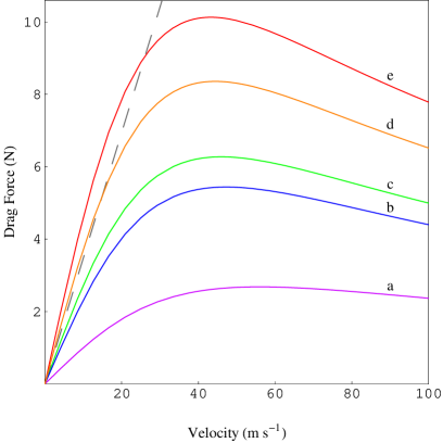
Figure 1: Plot of the drag force versus the magnet speed for a fixed value of the dipole moment and four different shape parameters $(L/2a,a/R_{1})$ (see the text for definitions): (a) typical cylinder, ($\frac{2}{1},0.60$), (b) “square” cylinder, ($\frac{1}{1},0.60$), (c) “point-like cylinder” ($\frac{1}{1},\simeq 0$), (d) short cylinder ($\frac{5}{8},0.96$), and (e) circular wafer, ($\simeq 0,\frac{3}{5}$). The dashed line represents the idealized limit.

The dashed line representing the idealized model corresponds to augmenting the point-dipole approximation by the thin-wall assumption, $(R_{2}-R_{1})/R_{1}\rightarrow 0$ thinwall . A comparison of the dashed line and curve (c) in Fig. 1 shows a relative deviation of about $10$% in the low-speed regime. This deviation should be compared with the ratio $(R_{2}-R_{1})/R_{1}$ characterizing the relative thickness of the pipe, which equals $0.100$ for all cases in Fig. 1. It is clear that the error caused by the thin-wall assumption is, in general, unacceptably large for a reasonable agreement with measurement results under typical conditions. Exceptions can of course occur: for case (d) corresponding to a short cylindrical magnet fitting snugly inside the pipe, the errors caused by the point-dipole and thin-wall approximations nearly cancel one another in the low-speed regime.

It is appropriate at this juncture to compare the prediction of our analysis to the measured results of MacLatchy et al. mac , bearing in mind the important caveat that the magnetization distribution in their experiment was not uniform. Using the parameter values reported by these authors, namely $m=0.67$ A ${\textrm{m}^{2}}$, $\sigma=5.08\times 10^{7}$ ${\Omega}^{-1}$ ${\textrm{m}}^{-1}$, $R_{1}=7.29$ mm, $R_{2}=7.96$ mm, $L=6.4$ mm, and $a=6.3$ mm, and equating their reported magnet (plus tape) weight of $0.060$ N to the magnetic drag force of Eq. (26) as well as setting ${\mu}_{rel}=1.00$ appropriate for copper, we find a magnet speed of $11.9\pm 0.5$ cm ${\textrm{s}}^{-1}$. MacLatchy et al. reported a measured terminal speed of $12.7\pm 0.4$ cm ${\textrm{s}}^{-1}$, and compared this to the prediction of the idealized model, $17.8$ cm ${\textrm{s}}^{-1}$. Note that in this comparison we are neglecting air drag on the magnet, estimated by the authors to be less than $0.1$% of the magnetic drag force hence deemed negligible. The quoted error of $0.5$ cm ${\textrm{s}}^{-1}$ in our calculated result is estimated on the basis of the (implied) precision level of the measured values given by MacLatchy et al. for $L$, $a$, $m$, $R_{2}-R_{1}$, and the magnet weight. Keeping in mind that the magnetization distribution of the “button” magnet used in the experiment was not uniform, and the fact that the drag force is rather sensitive to this distribution as demonstrated by the numerical modeling of MacLatchy et al., we conclude that our predicted value of the magnet speed agrees with the measured value within the uncertainties.

The circular wafer ($L=0$) geometry merits special attention since, in that case, the drag force grows without limit as $a\rightarrow R_{1}$. In other words, the shape characterized by ($0,1$) is a singular limit where the magnetic drag force diverges. This behavior may be understood as follows. In the limit of ($0,1$) geometry, the effective (or “bound”) source currents of the magnet are concentrated in a single current ring of radius $R_{1}$. However, such a source would induce similarly concentrated eddy current rings in the pipe wall on its interior surface, i.e., at zero distance from the source itself, thus causing infinite interaction forces due to overlapping current rings. This situation is analogous to the divergence of the image force on a point charge as it approaches the surface of a conductor. It is worth remarking that while the limit itself is unphysical, the sharp increase in the magnetic drag force for $L\ll a$ and $a\rightarrow R_{1}$ is very real and already discernible from a comparison of cases (c) and (e) in Fig. 1. In practice, this sharp increase in the magnetic drag would be accompanied by a parallel increase in the air drag force caused by the unavoidable constriction in the flow of air around the magnet vac .

The effect just discussed can also be understood in reference to Eq. (26). Using the asymptotic properties of the modified Bessel functions arfken , we find that $\textrm{Im}[Q(k)]\rightarrow\exp(-2kR_{1})/k$ as $k\rightarrow\infty$. Now for $L/a\rightarrow 0$ and $a\rightarrow R_{1}$, the shape factors in Eq. (26) behave like $\exp(2kR_{1})/k^{3}$ as $k\rightarrow\infty$. Putting these two statements together, we conclude that the integrand in Eq. (26) behaves like $k^{-1}$ for large $k$, which implies a logarithmic divergence at the upper limit of the integral. Recalling that $k$ is the Fourier conjugate of $z$ [cf. Eq. (26)], so that large values of $k$ are associated with short values of $z$, we conclude that this divergence is a short-distance effect. This is of course the conclusion we reached above on physical grounds.

V.2 Dependence on Magnet Speed

The dependence of the drag force on the speed of the magnet is contained in $Q(k)$ through the combination $\mu\sigma v$ and is more involved than the dependence on its shape. It proves expedient to discuss this dependence in terms of a length parameter defined by $l_{0}={({\mu}_{0}\sigma v)}^{-1}$. As discussed below, $l_{0}$ represents the penetration depth of the fields into the pipe wall under appropriate conditions. The two distinguished ranges of $v$, which we will refer to as “low” and “high” speed recall2 , correspond to $l_{0}\gg R_{1}$ and $l_{0}\ll R_{1}$, respectively tacit . We will first consider the low-speed regime, as it is the relevant one in practice. In this speed range, we have $\alpha\simeq 1-i/({\mu}_{rel}^{-1}l_{0}k)$, so that $\alpha kR_{1}\simeq kR_{1}-i(R_{1}/{\mu}_{rel}^{-1}l_{0})$, and similarly for $\alpha kR_{2}$. Thus the imaginary part of the argument of various modified Bessel functions is much smaller than the corresponding real part. This would in turn imply that, to the leading order, the imaginary part of those functions is linear in $R_{1}/l_{0}$ and $R_{2}/l_{0}$. This fact implies the same for $Q$, to wit, that in the low-speed regime the imaginary part of $Q$ is linear in $R_{1}/l_{0}$ (and $R_{2}/l_{0}$), hence proportional to $\sigma v$ mu . This confirms the expectation that in the low-speed regime where $l_{0}\gg R_{1}$, the braking force is a linear drag proportional to the conductivity of the pipe wall.

The linear nature of the drag force in the low-speed regime is in evidence for all cases in Fig. 1. In typical demonstration setups, one would expect terminal speeds of the order of $1\,\,\textrm{m}{\textrm{s}}^{-1}$ or less, which corresponds to the neighborhood of the origin in Fig. 1 where the drag force is closely proportional to the magnet speed. Indeed from the the low-speed condition $\mu\sigma vR_{1}\ll 1$ given above, we can estimate the relative deviation from linearity to be of the order of ${(\mu\sigma vR_{1})}^{2}$. For case (d) of Fig. 1, this estimate of deviation gives ${(0.63v[\textrm{m}\,{\textrm{s}}^{-1}])}^{2}$, which amounts to about $2.5$% at a terminal speed of $25$ m ${\textrm{s}}^{-1}$.

In the high-speed regime (which would require the projection of the magnet into the pipe with a suitably high initial speed) where $l_{0}\ll R_{1}$, we have $\alpha\simeq(1-i)/{(2{\mu}_{rel}^{-1}l_{0}k)}^{\frac{1}{2}}$ for values of $kR_{1}\approx 1$ which provide the main contribution to the integral in Eq. (26). This implies that $\alpha kR_{1}\simeq(1-i){(kR_{1}/2)}^{\frac{1}{2}}{(R_{1}/{\mu}_{rel}^{-1}l_{0})}^{\frac{1}{2}}$, and similarly for $\alpha kR_{2}$. Since $R_{1}/l_{0},R_{2}/l_{0}\gg 1$ in this speed range, the arguments of the modified Bessel functions in $Q$ which involve $\alpha$ will scale as ${(R_{1}/l_{0})}^{\frac{1}{2}}$ or ${(R_{2}/l_{0})}^{\frac{1}{2}}$ for $kR_{1}\approx 1$. Since these functions behave exponentially for large values of their argument, the said scaling behavior results in an overall suppression $\text{Im}(Q)$ in the high speed regime, corresponding to a decrease in the drag force. In other words, the drag force is a decreasing function of $\sigma v$ in the high-speed regime. Physically, a pronounced skin effect which suppresses the penetration of the field into the pipe wall takes hold at high speeds, thereby reducing the eddy currents and the drag force resulting from them. Indeed, recalling from section I.2 that the dominant time scale in the magnet-pipe system is $R_{1}/v$, which corresponds to a frequency $\omega\approx v/R_{1}$, we see that the high speed condition $l_{0}\ll R_{1}$ is equivalent to the inequality ${(\mu\sigma\omega)}^{-\frac{1}{2}}\ll R_{1}$ tacit . But this last condition states that the skin depth corresponding to the dominant time scale is much smaller than $R_{1}$ and, barring unusually thin-walled pipes, much smaller than $R_{2}-R_{1}$ as well. In other words, we have ${(\mu\sigma\omega)}^{-\frac{1}{2}}\ll R_{2}-R_{1}$ in this limit, which is the condition for a pronounced skin effect jackson . It is appropriate to repeat here that the high speed limit is not likely to occur in typical arrangements of the magnet-pipe demonstration.

The nonlinear behavior of the drag force at intermediate speeds and its eventual drop at high speeds deduced above are clearly in evidence for all cases displayed in Fig. 1. Note that the high-speed decline in the drag force becomes sharper as the source currents in the magnet are more highly concentrated. Recalling our discussion of the singular geometry above, we see the reason for this behavior: as source currents become more concentrated, short-distance, equivalently high-$k$, contributions become more important, a feature that runs contrary to the high-speed situation where high $k$ values are relatively less important.

V.3 Dependence on Conductivity and Susceptibility

Recall that the drag force dependence on the magnet speed is through the combination ${\mu}\sigma v$. This implies that the drag force behavior versus $\sigma$ follows the same pattern as for $v$. In particular, higher conductivity makes for a larger drag force at low speeds hence the use of copper tubes for demonstration purposes. At high speeds, however, the drag force decreases with pipe conductivity, just as it does with magnet speed. An interesting conclusion, therefore, is that the drag force vanishes for a perfect conductor which, as explained above, is simply a consequence of a strong skin effect. This behavior is displayed in Fig. 2, which is a plot of the drag force versus $\sigma$ for case (d) of section V.1 at a magnet speed of $0.10$ m ${\textrm{s}}^{-1}$. It is important to note that the decline of the drag force for high values of $\sigma$ is not directly applicable to practical arrangements which usually correspond to the low-speed (or possibly intermediate-speed) regime . Also to be noted is the fact that the designation “perfect conductor” here implies electric conduction without resistance, and is to be distinguished from “superconductor” which in addition implies a distinct magnetic behavior as noted below. Of course inasmuch as a superconductor has zero resistance, the above argument shows that the magnetic drag force vanishes for a superconducting pipe. Needless to say, this conclusion as well as the one above for a perfect conductor, directly follow from the energy conservation principle, which in this case asserts that there can be no drag force without a corresponding dissipation of power in the pipe.

Figure 2: Plot of the drag force versus the conductivity of the pipe for case (d) with $v=0.10$ m ${\textrm{s}}^{-1}$

.

This brings us to the question of how the magnetic properties of the pipe wall affect the drag force murel . Thus far we have assumed a linear magnetic material of relative permeability ${\mu}_{rel}$ for the pipe wall. Inasmuch as the magnetic susceptibility of non-ferromagnetic common metals differs little from that of the vacuum, one can set ${\mu}_{rel}\simeq 1$ for practical purposes, as we did for the cases displayed in Fig. 1. However, it is physically interesting and meaningful to consider the extreme cases of ${\mu}_{rel}\rightarrow 0$ and ${\mu}_{rel}\rightarrow\infty$, corresponding to perfect diamagnetism and perfect paramagnetism, respectively. Perfect diamagnetic behavior is exemplified by a (type I) superconductor which would exclude any magnetic field from its interior (save for a very small penetration depth). This phenomenon, known as the Meissner effect, is not a mere consequence of perfect conductivity and serves to distinguish a superconductor from a material that conducts electricity without dissipation ashmerm . Perfect paramagnetism, on the other hand, is approximately realized by “soft” ferromagnetic materials which have a narrow hysteresis loop and can be idealized as highly susceptible, linear magnetic materials.

An inspection of Eq. (26) shows that relative permeability occurs in the quantities $\alpha$ and $\beta=\alpha/{\mu}_{rel}$ through the combination ${\mu}_{rel}{\mu}_{0}\sigma v$ in $\alpha$, and in addition, $\beta$ is inversely proportional to ${\mu}_{rel}$. Leaving the latter aside for the moment, we conclude that the drag force dependence on ${\mu}_{rel}$ is much like its dependence on the magnet speed. Thus the drag force must vanish for both ${\mu}_{rel}\rightarrow 0$ and ${\mu}_{rel}\rightarrow\infty$, corresponding to strongly diamagnetic and paramagnetic limits. As further discussed in appendix D, the additional dependence of $\beta$ on ${\mu}_{rel}$ does not change these qualitative features. Thus the drag force corresponding to a superconductor vanishes not only because of its perfect conductivity but also due to its perfect diamagnetism. Similarly, the drag force is seen to be small for a strongly paramagnetic conductor, or soft ferromagnetic alloys that behave like one. The asymptotic behavior of the drag force for ${\mu}_{rel}\ll 1$ and ${\mu}_{rel}\gg 1$ is analyzed in appendices D and E, respectively, where the foregoing conclusions are explicitly confirmed.

Figure 3 shows a plot of the drag force versus ${\mu}_{rel}$ for case (d) of section V.1 at a magnet speed of $1.0$ m ${\textrm{s}}^{-1}$, where the features deduced above are in evidence.

Figure 3: Plot of the drag force versus the relative permeability of the pipe for case (d) with $v=1.0$ m ${\textrm{s}}^{-1}$

.

VI Concluding Remarks

The treatment of the magnet-pipe system in this paper has been based on axial symmetry. Therefore, any deviation of the magnet from a linear, axially centered motion such as wobbling or tumbling would violate this underlying assumption and cause a departure from the predicted results mu . Where necessary, the magnet can be placed inside an electromagnetically inactive casing with an optimum profile for stability. This procedure would also serve to maintain a fixed air drag coefficient when comparing magnets of different profile. Similarly, the analysis in this paper assumes an infinitely long pipe, so that in practice the magnet ends must be many times the interior pipe diameter away from the pipe ends when measurements are taken.

The results of this paper can be used for precision magnetic braking studies and applications. The computer program provided for use with this paper mathematica has been written for the case of uniform magnetization, but can readily be modified to deal with the general case using Eq. (25). For precision studies, it may be preferable to use an electromagnet instead of a permanent magnet, since the former allows a more convenient characterization of sources and fields.

Appendix A Low Magnet Speed

Here and in the following we will outline the development of a few limiting expressions for the drag force given in Eq. (26). The methods used are those of approximation and asymptotic analysis of integrals, the details of which would take us beyond the scope of this paper asympt .

As a preliminary step we recall that in all cases except for appendix D the main contributions to the integral of Eq. (26) originate from the region $k\simeq{R}_{1}^{-1}$. This fact makes it convenient to rescale the integration variable therein according to $k=u/R_{1}$. Effecting this substitution, we obtain

$$\mathbf{F}^{uni}=-\hat{\mathbf{v}}\frac{\mu_{0}m^{2}}{2{\pi}^{2}{R_{1}}^{4}}{\int}_{0}^{+\infty}duu^{3}{\left[\frac{\sin(uL/2R_{1})}{(uL/2R_{1})}\right]}^{2}{\left[\frac{{I}_{1}(ua/R_{1})}{(ua/2R_{1})}\right]}^{2}\textrm{Im}[Q(u,s/R_{1},{R_{1}}/l_{0},{\mu}_{rel})],$$ (30)

where we have explicitly defined the dependence of $Q$ on three dimensionless parameters which characterize the dimensions and material properties of the pipe as well as the magnet speed. Note that $s$ stands for the thickness of the pipe wall here. We shall use this representation to derive asymptotic expressions for the drag force in a number of interesting limiting cases.

The low-speed regime is defined by the condition ${R_{1}}/l_{0}\ll 1$ tacit . To establish the fact that $\mathbf{F}^{uni}$ is linear in $v$ in the low-speed limit, as discussed in Sec. V.2, we note that $Q(u,s/R_{1},0,{\mu}_{rel})$ is real at $v=0$ (corresponding to the vanishing of the drag force at zero speed), so that an expansion of $\textrm{Im}(Q)$ about $v=0$ using the asymptotic properties of the modified Bessel functions arfken yields $\textrm{Im}[Q(u,s/R_{1},{R_{1}}/l_{0},{\mu}_{rel})]\cong\mathcal{L}{R_{1}}/l_{0}$ for small ${R_{1}}/l_{0}$. The quantity $\mathcal{L}$ equals $\textrm{Im}[\partial Q(u,s/R_{1},0,{\mu}_{rel})/\partial({R_{1}}/l_{0})]$, and is given by a long expression which need not be reproduced here. Substituting the approximate form of Im(Q) in Eq. (30), we immediately obtain the linear drag behavior in the low-speed limit:

$${\mathbf{F}}^{lsp}\cong-\mathcal{C}\sigma v\hat{\mathbf{v}}\,\,\,({\mu}_{rel}{\mu}_{0}\sigma vR_{1}\ll 1),$$ (31)

where $\mathcal{C}$ depends on all parameters other than $\sigma$ and $v$.

Appendix B The Idealized Model

The idealized model involves three assumptions: (a) the point-dipole limit, $L/R_{1}\rightarrow 0,\,a/R_{1}\rightarrow 0$, (b) the low-speed approximation, ${R_{1}}/l_{0}\ll 1$, and (c) the thin-wall approximation, $s/R_{1}\ll 1$. The point-dipole limit is readily implemented by setting the two shape factors equal to unity. Items (b) and (c), on the other hand, require applying the thin-wall approximation to the quantity $\mathcal{C}$ introduced in Eq. (31). Using the properties of the modified Bessel functions, we find from Eqs. (18-20) that ${\mathcal{C}}\rightarrow(s/R_{1})u[{K}_{1}(u)]^{2}$. Therefore,

$${Q}^{idl}=i{\mu}_{0}(s/R_{1})u[{K}_{1}(u)]^{2}\sigma v,$$ (32)

where ${Q}^{idl}$ represents $Q$ in the ideal limit. Substituting this result in Eq. (30) (with the shape factors set to unity), we find

$${\mathbf{F}}^{idl}=-\frac{45{\mu}_{0}^{2}{m}^{2}s}{1024{R_{1}}^{4}}{\sigma}{v}\hat{\mathbf{v}},$$ (33)

in agreement with previous results saslow .

Appendix C High Magnet Speed

As stated in Sec. V.2, in the high-speed regime where $l_{0}/R_{1}\ll 1$, the quantity $\alpha$ in Eqs. (18-20) has a large magnitude which forces the respective modified Bessel functions to their asymptotic range. Since the four quantities $T_{ij}$ in Eqs. (19) have the same asymptotic limit arfken , they cancel out of Eq. (18). The remaining terms can then be simplified using the properties of the modified Bessel functions, leaving the result

$$\textrm{Im}({Q})\cong\frac{1}{kR_{1}}\frac{-\textrm{Im}(\beta)}{{[{I}_{0}(|k|R_{1})]}^{2}+|\beta|^{2}{[{I}_{1}(|k|R_{1})]}^{2}}\,\,\,({\mu}_{rel}{\mu}_{0}\sigma v\gg R_{1}).$$ (34)

The remaining $v$ dependence in Eq. 34 resides in $\beta=\alpha/{\mu}_{rel}$. Recalling from Sec. V.2 that $\alpha\rightarrow(1-i)/{(2{\mu}_{rel}^{-1}l_{0}k)}^{\frac{1}{2}}$ in the high-speed limit, we can reduce the above equation to tacit

$$\textrm{Im}({Q}) \cong \frac{\sqrt{{\mu}_{rel}}}{\sqrt{2k{\mu}_{0}\sigma v}R_{1}{[{I}_{1}(|k|R_{1})]}^{2}}$$ (35)

$$= \frac{\sqrt{{\mu}_{rel}}}{\sqrt{2uR_{1}/l_{0}}{[{I}_{1}(u)]}^{2}}\,\,\,({\mu}_{rel}{\mu}_{0}\sigma v\gg R_{1}).$$

Upon substituting this expression in Eq. 30, we find

$${\mathbf{F}}^{hsp}=-\frac{0.274m^{2}}{{R}_{1}^{9/2}}{\mathcal{F}}_{1}(a/R_{1},L/R_{1})\sqrt{\frac{{\mu}}{{\sigma v}}}\hat{\mathbf{v}},$$ (36)

where ${\mathcal{F}}_{1}$ is a form factor which depends on the dimensions of the magnet as fractions of the interior diameter of the pipe. It is defined by

$${\mathcal{F}}_{1}(a/{R_{1}},L/{R_{1}})=\frac{{{\mathcal{G}}_{1}}(a/{R_{1}},L/{R_{1}})}{{\mathcal{G}}_{1}(0,0)},$$ (37)

where

$${\mathcal{G}}_{1}(a/R_{1},L/R_{1})={\int}_{0}^{+\infty}du{u}^{5/2}{\left[\frac{\sin(uL/2R_{1})}{(uL/2R_{1})}\right]}^{2}{\left[\frac{{I}_{1}(ua/R_{1})}{(ua/2R_{1})}\right]}^{2}{[{I}_{1}(u)]}^{-2}.$$ (38)

Note that the form factor ${\mathcal{F}}_{1}$ has been normalized to unity at the point-dipole limit.

The asymptotic formula in Eq. (36) is valid in the high-speed limit ${\mu}_{rel}{\mu}_{0}\sigma v\gg R_{1}$ and describes the behavior of the drag force for very high magnet speed or pipe wall conductivity tacit .

Appendix D Highly Diamagnetic Pipe

This is the limit $\mu_{rel}\rightarrow 0$, which is appropriate to a highly diamagnetic pipe wall material. In this limit the factor $\beta$, which occurs in $Q$, grows large and severely suppresses the magnitude of $\textrm{Im}(Q)$ in Eq. (30), and in addition limits its contributions to very small values of $u$. This mathematical behavior reflects the physical phenomenon of magnetic flux expulsion that accompanies the approach to perfect diamagnetism.

Since only small values of $u$ are important in Eq. (30), we can replace all modified Bessel functions by their asymptotic values in the small argument limit arfken . This leads to the following approximate expression for $Q$:

$$Q=-\frac{{\alpha}^{2}\ln(R_{2}/R_{1})}{{\mu}_{rel}+\frac{1}{2}u^{2}\ln(R_{2}/R_{1}){\alpha}^{2}}.\,\,\,(u\ll 1)$$ (39)

Next, we find $\textrm{Im}(Q)$ and change the variable of integration in Eq. (30) according to $w={\mu}_{rel}^{-\frac{1}{2}}{\ln(R_{2}/R_{1})}^{\frac{1}{2}}\,u$. After some calculation and simplification, we find

$${\mathbf{F}}^{hdm}=-\mathcal{K}{\int}_{0}^{+\infty}d\zeta\,{\zeta}^{2}{[1+\frac{1}{2}{\zeta}^{2}]}^{-2}\hat{\mathbf{v}},$$ (40)

where

$$\mathcal{K}=\frac{{\mu}_{0}^{2}m^{2}\sigma v}{2{\pi}^{2}{R}_{1}^{3}}{[\ln(R_{2}/R_{1})]}^{-\frac{1}{2}}{\mu}_{rel}^{3/2}.$$ (41)

Finally, we carry out the integral in Eq. (40) to arrive at the asymptotic behavior of the drag force:

$${\mathbf{F}}^{hdm}=-\frac{{\mu}_{0}^{2}m^{2}\sigma v}{2{\pi}\sqrt{2}{R}_{1}^{3}}{[\ln(R_{2}/R_{1})]}^{-\frac{1}{2}}{\mu}_{rel}^{3/2}\,\hat{\mathbf{v}}.$$ (42)

The above formula is valid in the limit ${\mu}_{rel}\rightarrow 0$, and is appropriate to a highly diamagnetic pipe.

Appendix E Highly Paramagnetic Pipe

Here we are considering the limit $\mu_{rel}\rightarrow\infty$ appropriate to a highly susceptible pipe wall materialmurel . Recall from V.3 that the dependence of $Q$ on ${\mu}_{rel}$ occurs through the combination ${\mu}_{rel}{\mu}_{0}\sigma v$ in $\alpha$, and in addition through $\beta=\alpha/{\mu}_{rel}$. Consequently, Eq. 34 which is appropriate in the high-speed regime holds here as well. Recalling further that $\beta\rightarrow(1-i)/{(2{\mu}_{rel}l_{0}k)}^{\frac{1}{2}}$ in this limit, we find

$$\textrm{Im}({Q})\cong\frac{1}{\sqrt{2u^{3}l_{0}/R_{1}}{[{I}_{0}(u)]}^{2}\sqrt{{\mu}_{rel}}}\,\,\,({\mu}_{rel}\gg 1).$$ (43)

At this point we follow the steps subsequent to Eq. (34) to find

$${\mathbf{F}}^{hpm}=-\frac{0.0536{\mu}_{0}^{2}m^{2}}{{R}_{1}^{7/2}}{\mathcal{F}}_{0}(a/R_{1},L/R_{1})\sqrt{\frac{{\sigma v}}{{\mu}}}\hat{\mathbf{v}},$$ (44)

where ${\mathcal{F}}_{0}$ is a form factor which depends on the dimensions of the magnet as fractions of the interior diameter of the pipe. It is defined by

$${\mathcal{F}}_{0}(a/{R_{1}},L/{R_{1}})=\frac{{{\mathcal{G}}_{0}}(a/{R_{1}},L/{R_{1}})}{{\mathcal{G}}_{0}(0,0)},$$ (45)

where

$${\mathcal{G}}_{0}(a/R_{1},L/R_{1})={\int}_{0}^{+\infty}du{u}^{3/2}{\left[\frac{\sin(uL/2R_{1})}{(uL/2R_{1})}\right]}^{2}{\left[\frac{{I}_{1}(ua/R_{1})}{(ua/2R_{1})}\right]}^{2}{[{I}_{0}(u)]}^{-2}.$$ (46)

Note that the form factor ${\mathcal{F}}_{0}$ has been normalized to unity at the point-dipole limit.

The asymptotic formula given in Eq. (43) is valid in the limit ${\mu}_{rel}\gg 1$ and describes the behavior of the drag force for a highly susceptible pipe.

References

- (1) J. A. M. Clack and T. P. Toepker, Phys. Teach. 28, 236 (1990).
- (2) W. M. Saslow, Am. J. Phys. 60, 693 (1992).
- (3) C. S. Maclatchy, P. Backman, and L. Bogan, Am. J. Phys. 61, 1096 (1993).
- (4) K. D. Hahn, E. M. Johnson, A. Brokken, and S. Baldwin, Am. J. Phys. 66, 1066 (1998).
- (5) J. D. Jackson, Classical Electrodynamics, 3rd ed. (John Wiley, New York, 1999), pp. 218-220.
- (6) The SI system of units will be used throughout this paper.
- (7) A Mathematica program for computing the drag force as a function of velocity from Eq. (26) is provided for this purpose and may be downloaded from this URL: http://www.csus.edu/indiv/p/partovimh/magpipedrag.nb.
- (8) S. Weinberg, Gravitation and Cosmology (John Wiley, New York, 1972), pp. 67-70.
- (9) See Jackson jackson , p. 192.
- (10) Ibid., p. 554 et seq.
- (11) D. J. Griffiths, Introduction to Electrodynamics (Prentice Hall, New Jersey, 1999), third ed., p. 531.
- (12) Recall the discussion in the Sec. I.2 concerning the quasi-static limit.
- (13) See Jackson jackson , p. 126.
- (14) Ibid., Chapter 9.
- (15) The dipole radiation can be found from the magnetic dipole radiation formula, , where is the dipole moment in question. Using this formula, and recalling that the magnet’s dipole moment in the laboratory frame equals , we find the result . This quantity is in general smaller than the quadrupole radiation by a factor of order .
- (16) There is a zeroeth region, (), defined by , which we have not included here. The potential in this region is obtained from that in region (i) by substituting the appropriate representation of valid for . The latter is defined in the paragraph following Eq. (4).
- (17) It should be noted here that any deviation of from unity implies a repulsive (for ) or attractive (for ) radial force on the magnet should it deviate from a strictly axial motion. In the latter case (e.g., in the case of a magnet moving in an iron pipe), this force can easily destabilize the magnet unless it is constrained to move axially. We are grateful to David Jackson for reminding us of the practical importance of this effect.
- (18) G. B. Arfken and H. J. Weber, Mathematical Methods for Physicists, 5th ed. (Academic Press, San Diego, CA, 2001), Chapter 11.
- (19) The imaginary part of Q is positive, a fact that is not readily obvious from its definition.
- (20) An analogus situation obtains for the electrostatic force exerted on a charged object by its image with respect to a conducting or (linear) dielectric medium. Such a force would scale with the square of the real charge.
- (21) In effect the thin-wall approximation assumes uniform fields and eddy currents within the pipe wall thus ignoring the inevitable fall-off of all disturbances away from the axis. This is the reason why the thin-wall approximation in general overestimates the drag force.
- (22) Air drag effects can of course be eliminated by placing the pipe-magnet system in an evacuated chamber.
- (23) Recall that we have already restricted to nonrelativistic values.
- (24) Here we are implicitly assuming that is of the order of unity. We will consider departures from this assumption in V.3, and more specifically, the possibilites of and in appendices D and E, respectively.
- (25) Because the dependence of on is not just through the Bessel functions, this argument fails to give the full dependence of the force on .
- (26) N. W. Ashcroft and N. D. Mermin, Solid State Physics ((Holt, Rinehart, and Winston, New York, 1976), p. 731.
- (27) A general reference for asymptotic analysis is Norman Bleistein and Richard A. Handelsman, Asymptotic Expansions of Integrals (Dover Publications, New York, 1986); see also the textbook by Arfken and Weber arfken .
- (28) This is essentially the method of Green’s function for solving boundary value problems associated with linear systems; see, e.g., the textbook by Arfken and Weber arfken , or Jackson jackson , for a detailed description of this method.