Generic theory of active polar gels: a paradigm for cytoskeletal dynamics

Abstract

We develop a general theory for active viscoelastic materials made of polar filaments. This theory is motivated by the dynamics of the cytoskeleton. The continuous consumption of a fuel generates a non equilibrium state characterized by the generation of flows and stresses. Our theory can be applied to experiments in which cytoskeletal patterns are set in motion by active processes such as those which are at work in cells.

I Introduction

Molecular biology has scored an impressive number of success stories over the last forty years. It has provided us with a vast knowledge about molecules at work in living systems, about their involvement in specific biological functionalities and about the structure of their chemical networks albe02 . Yet one is still unable to take advantage of this knowledge for constructing a comprehensive description of cell behavior. Assuming that we had all desired molecular informations, the computer time required to describe meaningful cell behavior would be totally prohibitive. Meanwhile there is a clear need for a generic description of cells.

An alternative approach consists in identifying a reduced number of key characteristics and construct a phenomenological description of a ”simplified” but relevant cell. Again this task is currently too complex at the scale of a whole cell, but it can be envisioned for some of its constituents. A good example is provided by the description of membranes: for length scales of the order of a few tens of nanometers up, it can be considered as a fluctuating surface on which a few densities are distributed and through which a few other densities permeate passively or actively lipo95 ; mann01 . The construction of the theory has been going on for more than thirty years. It sheds light on the physics of membrane shape, topology changes such as budding, equilibrium and non equilibrium fluctuations, membrane adhesion, long range interactions on membranes etc… It is still under development to include out of equilibrium features such as lipid and protein exchange with the bulk, but much has been learned already.

Efforts towards understanding the cytoskeleton are more recent. They have been focused on the description of its passive visco-elastic properties which are now fairly well understood in terms of gels made of cross-linked semi-flexible polymers head03 ; wilh03 . Such materials which can be prepared in vitro, are equilibrium systems which obey conventional thermodynamics. In eukaryotic cells, the problem is however qualitatively new: the cross-links can be made of motor proteins which have their own dynamics driven by chemical energy. Experiments, simulations and analytical descriptions, have shown that such systems have a rich and complex behavior taki91 ; nede97 ; surr98 ; nede01 ; surr01 ; seki98 ; krus00 ; krus01 ; krus03 ; krus03a ; lee01 ; kim03 ; live03 . One can grasp the degree of complexity with the remark that cross-links define distances, in other words they define a metric. The cross-linking agents being motor proteins they move and the metric evolves with time.

In fact the problem is even more complex since cytoskeletal filaments are polar and out of equilibrium: they polymerize at one end while depolymerizing at the other end. Such a process called treadmilling is well known to biologists. The description of eukaryotic cytoskeletal gels should include all these features. We call these gels and more generally all gels working in the presence of a permanent energy consumption ”active” gels. On large length scales and long time scales, the properties of complex materials can be captured by a generalized hydrodynamic theory based on conservation laws and symmetry considerations. Such theories have been very successful in describing complex fluids such as liquid crystals, polymers, conventional gels, superfluids etc. mart72 ; dege70 ; seki91 . For instance all liquid crystal display devices can be described by such theories. More recently active liquid crystals have been considered within this same logic simh02 . Here, we develop a hydrodynamic theory of active gels. An example of such gel is the network of actin cytoskeletal filaments in the presence of chemical processes which locally induce filament sliding and generate motion. These active processes are mediated by motor proteins which hydrolyze a fuel, Adenosinetriphosphate (ATP). Since cytoskeletal filaments are structurally polar, each filament defines a vector. This filamental structure can on large scales give rise to a polarity of the material if filaments are aligned on average.

We develop the hydrodynamic theory of active polar gels systematically in several steps, following standard procedures. First, we identify the relevant fields and write conservation laws for conserved quantities. We identify the generalized fluxes and conjugate forces in the system. These fluxes and forces define the rates of entropy production and dissipation. Using the signature of forces and fluxes with respect to time reversal, we define dissipative and reactive fluxes. These fluxes can be expressed by a general expansion in terms of forces, by writing all terms allowed by symmetry and by respecting the signatures with respect to time reversal. By keeping the relevant terms to lowest order, this finally results in generic dynamic equations which are valid in the vicinity of thermal equilibrium. We then provide examples by analyzing the active gel mode structure and by discussing the spontaneous dynamical behavior of topological singularities such as disclinations (asters and vortices) in two dimensions. Eventually we discuss the merits of our approach, its current limitations and ways to extend its domain of validity to the more relevant far from equilibrium regime. Some of the results discussed here have been presented in Ref. krus04 .

II Fields, densities and conservation laws

We develop the hydrodynamic description of active gels starting with conservation laws. The number density of monomers in the gel is denoted by $\rho$. The gel is created by polymerization of filaments from monomers. The monomers have a density $\rho^{(a)}$ in solution. The treadmilling process and the active stresses in the gel create a flow of the actin gel monomers with a local velocity ${\bf v}$. The gel current is then convective and mass conservation implies that

$$\frac{\partial\rho}{\partial t}+\nabla{(\bf v\rho)}=-k_{d}\rho+k_{p}\delta_{S}$$ (1)

Here $k_{d}$ is the depolymerization rate; we assume, as seems to be the case for actin, that the depolymerization which occurs mostly at the branching points of the gel, has a rate proportional to the local density. In some cases treated below, we will consider for simplicity that depolymerization does not occur in the bulk but at the surface of the gel. In many situations, filament polymerization is highly controlled and localized for example at the surface of the gel. This is taken into account in Eq. (1) by introducing the surface polymerization rate $k_{p}$ and $\delta_{S}$ denotes a Dirac-like distribution which is non-vanishing only at the gel surface $S$. Similarly, we write a conservation law for free diffusing monomers,

$$\frac{\partial\rho^{(a)}}{\partial t}+\nabla{\bf j}^{(a)}=k_{d}\rho-k_{p}\delta_{S}$$ (2)

here, we have introduced the diffusive current ${\bf j}^{(a)}$ of free monomers.

Active processes are mediated by molecular motors. The concentration of motors bound to the gel $c^{(b)}$ is an important quantity to characterize the effects of active processes in the gel. Assuming for simplicity that the total number of motors is conserved, we write conservation laws for $c^{(b)}$ and the concentration of freely diffusing motors in the solvent $c^{(m)}$ which read

$$\frac{\partial c^{(m)}}{\partial t}+\nabla{\bf j}^{(m)} = k_{\rm off}c^{(m)}-k_{\rm on}\rho(c^{(m)})^{n}$$

$$\frac{\partial c^{(b)}}{\partial t}+\nabla c^{(b)}{\bf v}+\nabla{\bf j}^{(b)} = -k_{\rm off}c^{(b)}+k_{\rm on}\rho(c^{(m)})^{n}$$ (3)

The attachment and detachment rates of motors to and from the gel are characterized by the chemical rates $k_{\rm on}$ and $k_{\rm off}$. Here, we have taken into account that bound motors are convected with the gel. The current of free motors is ${\bf j}^{(m)}$ and we denote ${\bf j}^{(b)}$ the current of bound motors relative to gel motion. In general, binding of motors to the gel is cooperative, and cannot be described as a second order reaction: groups of motors could bind together. We use here an $n^{th}$ order chemical kinetics where the rates is proportional to $(c^{(m)})^{n}$.

A final important conservation law is momentum conservation. In biological gels on scales of micrometers, inertial forces are negligible and momentum conservation is replaced by the force balance condition which reads

$$\partial_{\alpha}(\sigma^{\rm tot}_{\alpha\beta}-\Pi\delta_{\alpha\beta})+f^{\rm ext}_{\beta}=0$$ (4)

where $f_{\beta}^{\rm ext}$ is an external force density. Locally, there are two forces acting on the gel, the total stress tensor $\sigma^{\rm tot}_{\alpha\beta}$ and the pressure $\Pi$.

The dynamics of the system is specified if the flow velocity ${\bf v}$ and the currents ${\bf j}^{(a)}$, ${\bf j}^{(m)}$ and ${\bf j}^{(b)}$ are known. The physical description of the currents is discussed in the following sections. Furthermore, we have to take into account the polar nature of the gel. Individual filaments are rod-like objects with two different ends which therefore have a vectorial symmetry. If the filaments in the gel are on average aligned, the material is oriented. We introduce a polarization field ${\bf p}$ to describe this orientation. The field $\bf p$ is defined by associating with each filament a unit vector pointing to one end. The vector ${\bf p}$ is given by the local average of a large number of these unit vectors.

III Constitutive equations

The fluxes of monomers and motor molecules are generated by forces which act on the active gel and induce motion. In this section, we identify the relevant forces and derive general flux-force relations. These relations define the material properties, and characterize how the system reacts to different types of generalized forces. Of particular significance for our theory is the existence of active processes mediated by molecular motors. In general, a chemical fuel, such as Adenosine-triphosphate ($ATP$), is used as an energy source. Motor molecules consume $ATP$ by catalyzing the hydrolysis to Adenosinediphosphate ($ADP$) and an inorganic phosphate and transduce the free energy of this reaction to generate forces and motion along the filaments. The energy of $ATP$ is also used for polymerization and depolymerization of the filaments. The presence of the fuel is equivalent to a chemical ”force” acting on the system. We characterize this generalized force by the chemical potential difference $\Delta\mu$ of $ATP$ and its hydrolysis products, $ADP$ and phosphate. When $\Delta\mu$ vanishes the chemical reaction is at equilibrium and there is no energy production. When $\Delta\mu>0$, a free energy $\Delta\mu$ is consumed per hydrolyzed $ATP$ molecule.

Constitutive equations are obtained by first identifying the fluxes and the corresponding conjugate generalized forces and then writing a general expansion for the fluxes in terms of the forces. We study in this paper an active gel close to thermodynamic equilibrium and limit the expansion of fluxes in terms of forces to linear order as in a standard Onsager theory. We thus describe the linear response of the gel to generalized forces. We do this in the most general way and write in the flux-force expansion all terms which are consistent with the symmetries of the system.

III.1 Fluxes and forces

We first discuss the rate of entropy production in the active gel. A change in the free energy $F=U-TS$ per unit time can be written as

$$\dot{F}=-\int d^{3}{\bf r}\left\{\sigma^{\rm tot}_{\alpha\beta}\partial_{\alpha}v_{\beta}+h_{\alpha}\dot{p}_{\alpha}+\Delta\mu r+\partial_{\alpha}j_{\alpha}^{(i)}\mu^{(i)}\right\}$$ (5)

where the “dot” denotes a time derivative. The total deviatory stress tensor $\sigma^{\rm tot}_{\alpha\beta}$ is in general is not symmetric; it is conjugate to the velocity gradient $\partial_{\alpha}v_{\beta}$. The field conjugate to the order parameter $p_{\alpha}$ is the functional derivative of the free energy $F$ of the gel at thermal equilibrium, $h_{\alpha}=-\frac{\delta F}{\delta p_{\alpha}}$, where the functional derivative is taken for constant deformation, temperature and number of particles. The current conjugate to the field $h_{\alpha}$ is the convected time derivative of the polarization $\dot{p}_{\alpha}=\frac{\partial p_{\alpha}}{\partial t}+v_{\beta}\partial_{\beta}p_{\alpha}$. The chemical force $\Delta\mu$ is conjugate to the $ATP$ consumption rate $r$ which determines the number of $ATP$ molecules hydrolyzed per unit time and per unit volume. Finally, $\mu^{(a)}$, $\mu^{(m)}$ and $\mu^{(b)}$ are the chemical potentials of free monomers, free motors and of motors bound to the gel, respectively.

Eq. (5) does not take into account the translational and rotational invariance of the active gel, and the variables used are therefore not the proper conjugate fluxes and forces. Indeed, as shown in reference dege93 , since the free energy does not change under pure translations and rotations of the gel, ignoring surface terms, we can rewrite Eq. (5) as

$$\dot{F}=-\int d^{3}{\bf r}\left\{\sigma_{\alpha\beta}u_{\alpha\beta}+h_{\alpha}P_{\alpha}+\Delta\mu r-j_{\alpha}^{(i)}\partial_{\alpha}\mu^{(i)}\right\}$$ (6)

The total stress $\sigma^{\rm tot}$ has been decomposed into a symmetric part $\sigma_{\alpha\beta}$ (with $\sigma_{\alpha\beta}=\sigma_{\beta\alpha}$) and and anti-symmetric part which is due to the torque exerted by the field $h_{\alpha}$ on the order parameter $p_{\alpha}$:

$$\sigma^{\rm tot}_{\alpha\beta}=\sigma_{\alpha\beta}+\frac{1}{2}(p_{\alpha}h_{\beta}-p_{\beta}h_{\alpha})$$ (7)

Here, $u_{\alpha\beta}=\frac{1}{2}(\partial_{\alpha}v_{\beta}+\partial_{\beta}v_{\alpha})$ is the symmetric part of the velocity gradient tensor. The current conjugate to $h_{\alpha}$ includes a rotational contribution coming from the antisymmetric part of the stress tensor, it reads

$$P_{\alpha}=\frac{D}{Dt}p_{\alpha}=\frac{\partial p_{\alpha}}{\partial t}+(v_{\gamma}\partial_{\gamma})p_{\alpha}+\omega_{\alpha\beta}p_{\beta}$$ (8)

where we have used the corotational time derivative of the vector $p_{\alpha}$, $\omega_{\alpha\beta}=\frac{1}{2}(\partial_{\alpha}v_{\beta}-\partial_{\beta}v_{\alpha})$ being the vorticity tensor of the flow.

We can read off Eq. (6) the following pairs of conjugate fluxes and forces:

flux $$\leftrightarrow$$ force

$$\sigma_{\alpha\beta} \leftrightarrow u_{\alpha\beta}$$

$$P_{\alpha} \leftrightarrow h_{\alpha}$$ (9)

$$r \leftrightarrow \Delta\mu$$

$$j_{\alpha}^{(i)} \leftrightarrow \partial_{\alpha}\mu^{(i)}$$

The rate of change of the free energy can be divided into reversible and irreversible parts $\dot{F}=\dot{F}_{\rm rev}+\dot{F}_{\rm irr}$ where $\dot{F}_{\rm rev}=\dot{U}$ and $\dot{F}_{\rm irr}=-T\dot{S}$. We therefore decompose the fluxes into a reactive part and a dissipative part. They are characterized by their different signatures with respect to time-reversal. Note, that the generalized forces have well-defined signatures with respect to time reversal: the rate of strain $u_{\alpha\beta}$ is odd under time reversal, while $h_{\alpha}$ and $\Delta\mu$ are even. We write

$$\sigma_{\alpha\beta} = \sigma_{\alpha\beta}^{r}+\sigma_{\alpha\beta}^{d}$$

$$P_{\alpha} = P_{\alpha}^{r}+P_{\alpha}^{d}$$

$$r = r^{r}+r^{d}\quad.$$ (10)

The dissipative fluxes have the same signature under time reversal as their conjugate forces, while reactive fluxes have the opposite signature under time reversal. Therefore, $\sigma^{d}_{\alpha\beta}$ is odd under time reversal, while $r^{d}$ and $P_{\alpha}^{d}$ are even. The reactive parts have correspondingly the opposite signatures. As we show below, the currents $j^{(i)}_{\alpha}$ do not have reactive parts. With this decomposition, the rate of entropy production $T\dot{S}=-\dot{F}_{\rm irr}$ is given by

$$T\dot{S}=\int d^{3}{\bf r}\left\{r^{d}\Delta\mu+P_{\alpha}^{d}h_{\alpha}+\sigma^{d}_{\alpha\beta}u_{\alpha\beta}-j_{\alpha}^{(i)}\partial_{\alpha}\mu^{(i)}\right\}\quad.$$ (11)

For a changing state of the system which is periodic in time with period $T$, the internal energy is the same after one period. Therefore, in this case

$$\int_{0}^{T}dt(r^{r}\Delta\mu+P_{\alpha}^{r}h_{\alpha}+\sigma^{r}_{\alpha\beta}u_{\alpha\beta})=0\quad.$$ (12)

These relations follow from the signatures of dissipative and reactive currents under time reversal.

III.2 Maxwell model

In the absence of a net gel polarization ${\bf p}$ and for a passive system with $\Delta\mu=0$, we describe the viscoelastic gel by a Maxwell model. In order to keep our expressions simple and to focus on the essential physics, we assume that the ratio of the bulk and shear viscosities is $2/d$ where $d$ is the space dimension. The Maxwell model relates the stress tensor to the strain rate according to

$$\left(1+\tau\frac{D}{Dt}\right)\sigma_{\alpha\beta}=2\eta u_{\alpha\beta}$$ (13)

Here, $\eta$ denotes the shear viscosity and $\tau$ the viscoelastic relaxation time. and $E=\eta/\tau$ is the elastic modulus of the gel at short times. In Eq. (13), the time derivative of the stress tensor taken in a reference frame moving with the material flow must be used. For a tensor, this implies that in the laboratory frame convective terms due to the fluid flow as well as the rotation of the reference system due to the vorticity of the flow need to be taken into account. $D/Dt$ denotes the corotational derivative of a tensor given by

$$\frac{D\sigma_{\alpha\beta}}{Dt}\equiv\frac{\partial\sigma_{\alpha\beta}}{\partial t}+(v_{\gamma}\partial_{\gamma})\sigma_{\alpha\beta}+\left[\omega_{\alpha\gamma}\sigma_{\gamma\beta}+\omega_{\beta\gamma}\sigma_{\gamma\alpha}\right]$$ (14)

Note that we include the geometrical non-linearities and that we use the most general versions of what is called a “Convected Maxwell Model” bird87 . For the Maxwell model given by Eq. (13), we can specify the reactive and the dissipative contributions to the stress tensor.

$$(1-\tau^{2}\frac{D^{2}}{Dt^{2}})\sigma_{\alpha\beta}^{d} = 2\eta u_{\alpha\beta}$$ (15)

$$\sigma_{\alpha\beta}^{r} = -\tau\frac{D}{Dt}\sigma_{\alpha\beta}^{d}$$ (16)

With these relations, we have $\sigma_{\alpha\beta}=\sigma_{\alpha\beta}^{d}+\sigma_{\alpha\beta}^{r}$ and the dissipative and reactive parts of the stress differ in their signature with respect to time reversal.

III.3 Dissipative fluxes

We now generalize the relations (15) and (16) expressing dissipative and reactive fluxes in terms of generalized forces for an active polar gel. First, we write expressions for the dissipative fluxes. To linear order we find

$$\left(1-\tau^{2}\frac{D^{2}}{Dt^{2}}\right)\sigma_{\alpha\beta}^{d} = 2\eta u_{\alpha\beta}$$ (17)

$$- \tau\frac{D}{Dt}(\frac{\nu_{1}}{2}(p_{\alpha}h_{\beta}+p_{\beta}h_{\alpha})+\bar{\nu}_{1}p_{\gamma}h_{\gamma}$$

$$\left(1-\tau^{2}\frac{D^{2}}{Dt^{2}}\right)P^{d}_{\alpha} = \left(1-\tau^{2}\frac{D^{2}}{Dt^{2}}\right)(\frac{h_{\alpha}}{\gamma_{1}}+\lambda_{1}p_{\alpha}\Delta\mu)$$ (18)

$$+ \tau\frac{D}{Dt}(\nu_{1}p_{\beta}u_{\alpha\beta}+\bar{\nu}_{1}p_{\alpha}u_{\beta\beta})$$

$$r^{d} = \Lambda\Delta\mu+\lambda_{1}p_{\alpha}h_{\alpha}+\lambda p_{\alpha}\partial_{\alpha}\mu^{(b)}\quad.$$ (19)

Note that the first expression is a generalization for Eq. (15) of the Maxwell model. For a sake of simplicity, we ignore the anisotropy of the viscosity and consider that all translational viscosities are equal. This anisotropy could be introduced as in the classical description of the hydrodynamics of liquid crystals. Couplings to $\Delta\mu$ cannot appear in the equation of the dissipative stress because it transforms differently under time reversal than $u_{\alpha\beta}$. A term coupling $\sigma_{\alpha\beta}^{d}$ to the time derivative of $h_{\alpha}$ can appear. It is required by Onsager symmetry relations since a corresponding coupling term with coefficient $\nu_{1}$ does occur in the equation for $P^{d}_{\alpha}$ as shown in Appendix B. The dissipative coefficients $\gamma_{1}$ and $\Lambda$ characterize the coupling of $P^{d}_{\alpha}$ and $r^{d}$ to $h_{\alpha}$ and $\Delta\mu$, respectively. Here, $\gamma_{1}$ is the rotational viscosity which appears in classical nemato-hydrodynamics. Because of its signature with respect to time reversal, cross-coupling terms involving $u_{\alpha\beta}$ do not appear in the expression $r^{d}$. The expression for $P^{d}_{\alpha}$ contains a terms coupling $P^{d}_{\alpha}$ to the time derivative of $u_{\alpha\beta}$ as derived in Appendix B. Cross-coupling terms occur also in the expressions for $P^{d}_{\alpha}$ and $r^{d}$. Since $P_{\alpha}$ is a vector and $r$ a scalar, we need a vector in the system to couple these equations. If the system is polar, this vector is provided by ${\bf p}$. Therefore, the cross-coupling term characterized by $\lambda_{1}$ involves $p_{\alpha}$. Note that because of the symmetry of the Onsager coefficients, the coefficients $\lambda_{1}$ $\nu_{1}$ and $\bar{\nu}_{1}$ are the same in different equations. The last term in the expression of $r^{d}$ is a crossed term with the current of bound motors discussed below. This term is also imposed by the Onsager symmetry relations. We still have to specify the currents $j^{(a)}_{\alpha}$, $j^{(m)}_{\alpha}$ and $j^{(b)}_{\alpha}$ of monomers and motor molecules which do not have reactive components:

$$j_{\alpha}^{(a)} = -D^{(a)}\partial_{\alpha}\rho^{(a)}$$ (20)

$$j_{\alpha}^{(m)} = -D^{(m)}\partial_{\alpha}c^{(m)}$$ (21)

$$j_{\alpha}^{(b)} = -D^{(b)}\partial_{\alpha}c^{(b)}+\lambda p_{\alpha}\Delta\mu$$ (22)

The first two expressions are simple diffusive currents with diffusion coefficients $D^{(i)}$, where we have assumed for simplicity that couplings to $h_{\alpha}$ can be neglected and that free diffusion is not influenced by $\Delta\mu$. The expression (22) describes bound motors which are convected with the gel. In addition to being convected with velocity ${\bf v}$, motors move in a direction given by the filament orientation if $\Delta\mu$ is nonzero. This directed motion is characterized by the coefficient $\lambda$; the motor velocity $v^{m}$ on the filaments is such that $c^{(b)}v^{m}_{\alpha}=\lambda p_{\alpha}\Delta\mu$. Finally, velocity fluctuations of motor motion are captured by a diffusive term with diffusion constant $D^{(b)}$.

III.4 Reactive fluxes

Reactive fluxes are expressed in terms of the forces following their signature under time translation invariance. Generalizing Eq.(16) for the reactive stresses of the Maxwell model, we note that here cross coupling terms with the forces $h_{\alpha}$ and $\Delta\mu$ are possible. Taking into account the tensorial structure of the stress tensor, we write

$$\sigma_{\alpha\beta}^{r} = -\tau\left[\frac{D\sigma_{\alpha\beta}^{d}}{Dt}+A_{\alpha\beta}\right]-\zeta\Delta\mu p_{\alpha}p_{\beta}-\bar{\zeta}\Delta\mu\delta_{\alpha\beta}$$ (23)

$$- \zeta^{\prime}\Delta\mu p_{\gamma}p_{\gamma}\delta_{\alpha\beta}$$

$$+ \frac{\nu_{1}}{2}(p_{\alpha}h_{\beta}+p_{\beta}h_{\alpha})+\bar{\nu}_{1}p_{\gamma}h_{\gamma}\delta_{\alpha\beta}\quad,$$

where we have introduced the phenomenological coefficients $\zeta$, $\bar{\zeta}$, $\zeta^{\prime}$, $\nu_{1}$ and $\bar{\nu}_{1}$. The tensor

$$A_{\alpha\beta} = \nu_{2}(u_{\alpha\gamma}\sigma_{\gamma\beta}^{d}+\sigma_{\alpha\gamma}^{d}u_{\gamma\beta})+\nu_{3}u_{\gamma\gamma}\sigma_{\alpha\beta}^{d}+\nu_{4}u_{\gamma\gamma}\sigma_{\delta\delta}^{d}\delta_{\alpha\beta}$$ (24)

$$+ \nu_{5}\sigma_{\gamma\gamma}^{d}u_{\alpha\beta}+\nu_{6}u_{\gamma\delta}\sigma_{\delta\gamma}^{d}\delta_{\alpha\beta}\quad.$$

contains nonlinear reactive terms to lowest order, resulting from the geometry of the flow field with corresponding phenomenological coefficients $\nu_{i}$. Similar coefficient have been introduced in the so-called “eight constant Oldroyd model” in rheology bird87 . The term proportional to $\tau$ on the right hand side of Eq. (23) assures compatibility with the Maxwell model in the absence of polarization and chemical fuel. For the reactive parts of $P_{\alpha}$ and $r$ we write

$$(1-\tau^{2}\frac{D^{2}}{Dt^{2}})P_{\alpha}^{r} = -\nu_{1}u_{\alpha\beta}p_{\beta}-\bar{\nu}_{1}u_{\beta\beta}p_{\alpha}$$ (25)

$$r^{r} = \zeta p_{\alpha}p_{\beta}u_{\alpha\beta}+\bar{\zeta}u_{\alpha\alpha}+\zeta^{\prime}p_{\alpha}p_{\alpha}u_{\beta\beta}$$ (26)

Here we have written cross coupling terms of $P^{r}$ with the rate of strain $u_{\alpha\beta}$. The linear response matrix of reactive terms is antisymmetric, therefore the same coefficients as in Eq. (23) appear, however with opposite sign. The remaining Eq. (26) is constructed in the same way with cross coupling coefficients that have been introduced in Eq. (23). No reactive cross-terms between Eqns. (25) and (26) exist.

III.5 Dynamic equations

Using the expressions for dissipative and reactive fluxed discussed above, we now write general hydrodynamic equations for the active viscoelastic and polar gel. Adding the dissipative and reactive parts, we find

$$2\eta u_{\alpha\beta} = \left(1+\tau\frac{D}{Dt}\right)\left\{\sigma_{\alpha\beta}+\zeta\Delta\mu p_{\alpha}p_{\beta}\right.$$ (27)

$$\left.+\zeta^{\prime}\Delta\mu p_{\gamma}p_{\gamma}\delta_{\alpha\beta}+\bar{\zeta}\Delta\mu\delta_{\alpha\beta}+\tau A_{\alpha\beta}\right\}$$

$$- \frac{\nu_{1}}{2}(p_{\alpha}h_{\beta}+p_{\beta}h_{\alpha})-\bar{\nu}_{1}p_{\gamma}h_{\gamma}\delta_{\alpha\beta}$$

$$\left(1-\tau^{2}\frac{D^{2}}{Dt^{2}}\right)\frac{Dp_{\alpha}}{Dt} = \left(1-\tau^{2}\frac{D^{2}}{Dt^{2}}\right)(\frac{1}{\gamma_{1}}h_{\alpha}+\lambda_{1}p_{\alpha}\Delta\mu)$$ (28)

$$-(1-\tau\frac{D}{Dt})(\nu_{1}u_{\alpha\beta}p_{\beta}+\bar{\nu}_{1}u_{\beta\beta}p_{\alpha})$$

$$r = \zeta p_{\alpha}p_{\beta}u_{\alpha\beta}+\bar{\zeta}u_{\alpha\alpha}+\zeta^{\prime}p_{\alpha}p_{\alpha}u_{\beta\beta}$$ (29)

$$+ \Lambda\Delta\mu+\lambda_{1}p_{\alpha}h_{\alpha}\quad.$$

In these equations, we have included geometric nonlinearities but have restricted other terms to linear order for simplicity. Also, we have neglected chiral terms which in principle exist in cytoskeletal systems but which are expected to be small. These equations are complemented by the force balance condition (4).

Eq. (27) generalizes the expression of the stress tensor in the Maxwell model to active systems with polarity. Indeed, even in the absence of stresses, the active terms proportional to $\Delta\mu$ generate a finite strain rate. Similarly, if all flows are suppressed, the active terms generate a nonzero stress tensor. Thus, the hydrolysis of $ATP$ can generate forces and material flow in the gel via the action of active elements such as motors. These terms are characterized by the coefficients $\zeta$, $\zeta^{\prime}$ and $\bar{\zeta}$ Similarly, we find active terms in the polarization dynamics given by Eq. (28) described by the coefficient $\lambda_{1}$. Furthermore, material flow couples to the polarization dynamics via the coefficients $\nu_{1}$ and $\bar{\nu}_{1}$. The rate of $ATP$ consumption $r$ is primarily driven by $\Delta\mu$ and characterized by $\Lambda$. However, it is also coupled to the fluid flow and to the field ${\bf h}$ acting on $\bf p$. Note, that in addition surface terms can be important. For example, if filaments polymerize at the gel surface with a rate $k_{p}$ (see Eq. (1)), there is an additional contribution $r_{S}$ to ATP consumption which is localized at the surface. In the following, we discuss situation where surface effects can be captured by introducing appropriate boundary conditions.

IV Hydrodynamic modes

We now calculate the linear relaxation modes of an active polar gel. They can be obtained from the linear response of the change in the gel density to externally applied forces. We focus on the situation of a fully polarized gel far from an isotropic polar transition with the polarization vector lying in the $x$-direction, i.e., ${\bf p}={\bf e}_{x}$ is constant. We assume that the gel is treadmilling, which implies that it moves at constant velocity ${\bf v}=v_{0}{\bf e}_{x}$, while the gel mass is conserved. The treadmilling is due to polymerization and depolymerization of the filaments at the gel surfaces located at $x=x^{+}$ and $x=x^{-}$, respectively. In the following, we consider the case of an infinite system where $x^{+}$ are located at $+\infty$ and $x^{-}$ to $-\infty$ while the treadmilling velocity $v_{0}$ remains constant.

We restrict ourselves to modes for which the fields vary along the $x$-direction which is the treadmilling direction, while the system is assumed to be homogeneous in the other directions. In this case the dynamic equations (1)-(3) for the densities of polymerized actin, bound and free myosin become effectively one-dimensional and read

$$\partial_{t}\rho+\partial_{x}(\rho v) = 0$$ (30)

$$\partial_{t}c^{(m)}-D\partial_{x}^{2}c^{(m)} = k_{\rm off}c^{(b)}-k_{\rm on}\rho(c^{(m)})^{n}$$ (31)

$$\partial_{t}c^{(b)}+\partial_{x}(c^{(b)}v+\lambda\Delta\mu) = -k_{\rm off}c^{(b)}+k_{\rm on}\rho(c^{(m)})^{n}\quad.$$ (32)

The actin monomers which are not part of the gel diffuse across the system and control by their concentrations the treadmilling rate. The mechanical constitutive equation (27) takes the form

$$2\eta\partial_{x}v=[1+\tau\partial_{t}+\tau v\partial_{x}](\sigma+\zeta\Delta\mu)$$ (33)

whereas the force balance in the presence of an external stress $\sigma^{\rm ext}$ is expressed by

$$\partial_{x}(\sigma+\sigma^{\rm ext})=\partial_{x}\Pi\quad.$$ (34)

In these equations, the coefficients $\lambda$ and $\zeta$, which are the Onsager coefficients introduced in the previous section, characterize the directed motion of motors along the filaments and the actively generated stress in the gel (we have replaced here $\zeta+\zeta^{\prime}+\bar{\zeta}$ by $\zeta$.). In a situation far from equilibrium, nonlinearities become important. We therefore linearize around the homogeneous steady state of the above equations given by $\rho=\rho_{0}$, $c^{(b)}=c^{(b)}_{0}$, $c^{(m)}=c^{(m)}_{0}$, $v=v_{0}$, and $\sigma=\sigma_{0}$, where $k_{\rm off}c^{(b)}_{0}=k_{\rm on}\rho_{0}(c^{(m)}_{0})^{n}=\rho_{0}v_{0}$ and $\sigma_{0}=-\zeta\Delta\mu$. We consider a small perturbation of this state, i.e., $\rho=\rho_{0}+\delta\rho$ and analogously for the remaining quantities. To leading order, the active coefficients can be expanded as $\zeta=\zeta_{0}+\zeta_{\rho}\delta\rho+\zeta_{c}\delta c^{(b)}$ and $\lambda=\lambda_{0}+\lambda_{\rho}\delta\rho+\lambda_{c}\delta c^{(b)}$ to implement such nonlinearities which become relevant in all realistic situations. Here, we have neglected the diffusion of bound motors and the diffusion constant $D^{(b)}$ has been set to zero.

The linearized dynamical equations can be solved by Fourier-transformation in space and time. The mode characterizing the variations of the density of unbound motors, $c^{(m)}(q,\omega)$ as a function of spatial wave vector $q$ and temporal frequency $\omega$, can be obtained from Eq. (31) and is given by

$$c^{(m)}(q,\omega)=\frac{k_{\rm off}c^{(b)}(q,\omega)-k_{\rm on}(c^{(m)}_{0})^{n}\rho(q,\omega)}{i\omega+Dq^{2}+T_{c}^{-1}}\quad,$$ (35)

where $T_{c}^{-1}=nk_{\rm on}\rho_{0}(c^{(m)}_{0})^{n-1}$ is a chemical relaxation time. Using this result as well as the linearized conservation equation

$$i\omega\rho(q,\omega)+iq\rho_{0}v(q,\omega)+iqv_{0}\rho(q,\omega)=0$$ (36)

we obtain for the distribution of bound motors

$$c^{(b)}(q,\omega)=\frac{A(q,\omega)c_{0}-iq\bar{\lambda}_{\rho}}{A(q,\omega)+iq\bar{\lambda}_{c}}\frac{\rho(q,\omega)}{\rho_{0}}$$ (37)

where $\bar{\lambda}_{\rho}=\lambda_{\rho}\Delta\mu\rho_{0}$, $\bar{\lambda}_{c}=\lambda_{c}\Delta\mu$, and

$$A(q,\omega)=i\omega+iqv_{0}+\frac{i\omega+Dq^{2}}{i\omega+Dq^{2}+T_{c}^{-1}}k_{\rm off}\quad.$$ (38)

The mechanical equations (33) and (34) then lead to

$$\sigma^{\rm ext}(q,\omega)=2\mu(q,\omega)\frac{\rho(q,\omega)}{\rho_{0}}$$ (39)

where the modulus $\mu(q,\omega)$ characterizes the effective material properties in response to density variations. It can be determined from the Eq.

$$(1+i\tau(\omega+qv_{0}))\left[2\mu(q,\omega)-\chi\rho_{0}\right]=2iE\tau(\omega+qv_{0})$$

$$+(1+i\omega\tau+iqv_{0}\tau)\left[\bar{\zeta}_{\rho}+\bar{\zeta}_{c}\frac{A(q,\omega)c_{0}-iq\bar{\lambda}_{\rho}}{A(q,\omega)+iq\bar{\lambda}_{c}}\right]\quad.$$ (40)

Here, we have used the equation of state and have defined the inverse compressibility $\chi=\frac{\partial\Pi}{\partial\rho}$. Furthermore, we have introduced $\bar{\zeta}_{\rho}=\zeta_{\rho}\Delta\mu\rho_{0}$ as well as $\bar{\zeta}_{c}=\zeta_{c}\Delta\mu$.

The relaxation modes of the system can be identified by the (complex) values of the frequency $\omega_{n}$, for which the modulus vanishes $\mu(q,\omega_{n})=0$. Indeed, the density relaxes as $\rho(q)\sim e^{i\omega_{n}t}$ and instabilities in the system occur if the real part of $i\omega_{n}$ becomes positive. For our present system, we find that three independent relaxation modes exist, with $n=1$ to $3$. Up to leading order in $q$, the corresponding dispersion relations are given by

$$i\omega_{1} = icq+dq^{2}$$ (41)

$$i\omega_{2} = -T_{c}^{-1}-k_{\rm off}$$ (42)

$$i\omega_{3} = -\frac{1}{\tau}\frac{\chi\rho_{0}+\bar{\zeta}_{c}c_{0}+\bar{\zeta}_{\rho}}{2E+\chi\rho_{0}+\bar{\zeta}_{c}c_{0}+\bar{\zeta}_{\rho}}$$ (43)

The first mode is propagating with velocity $c$ given by

$$c=-\frac{1}{1+T_{c}k_{\rm off}}\left[v_{0}+\frac{(\chi\rho_{0}+\bar{\zeta}_{\rho})\bar{\lambda}_{c}-\bar{\zeta}_{c}\bar{\lambda}_{\rho}}{\chi\rho_{0}+\bar{\zeta}_{\rho}+\bar{\zeta}_{c}c_{0}}\right]$$ (44)

Note, that the propagation velocity $c$ is proportional to the fraction of bound motors $(1+T_{c}k_{\rm off})^{-1}$. The value of the coefficient $d$ can be either positive or negative, depending on the value of the parameters. If it is positive, the gel is unstable and self-organizes into propagating density profiles. Such solitary waves have been found in theoretical descriptions of active polar fibers krus01 ; krus03 . Experimentally, actin waves have been recently reported in several cell types vick02 ; bret04 ; gian04 . In the present context, there is only one propagating mode, because space inversion symmetry has been broken due to treadmilling and to the polarization of the gel. The polarization couples to the filament and motor densities only through the active current of bound motors. If instead of motors, we have passive cross-linkers, i.e., $\lambda=0$ and in the absence of treadmilling, i.e., $v_{0}=0$, space inversion symmetry is restored. In this case $c=0$ and

$$d=-D\frac{k_{\rm off}}{T_{c}^{-1}+k_{\rm off}}\quad,$$ (45)

so that the mode is no longer propagating, but diffusive and always stable. Note, that $d$ is proportional to the fraction of unbound motors $T_{c}k_{\rm off}/(1+T_{c}k_{\rm off})$. The existence of propagating waves even in a viscous environment seems to be a general feature of active media and has already been reported in an other context by Ramaswamy and coworkers rama00 ; simh02 .

The second mode is a chemical relaxation mode describing the binding and unbinding of molecular motors to the polymerized gel, whereas the third mode describes the stress relaxation towards its stationary value.

V Dynamic point defect in two dimensions

As an example of active behavior in two dimensions described by Eqns. (29), we consider in this section the dynamics of point defects in the vector field ${\bf p}$. First, we consider the passive equilibrium state with $\Delta\mu=0$ where all fluxes vanish. Subsequently, we determine stationary active solutions for finite $\Delta\mu$ and determine their stability. We obtain a complete diagram of states for asters, vortices and rotating spirals.

V.1 Asters and vortices at thermodynamic equilibrium

In order to study point defects in two dimension, we consider for simplicity the situation where the orientation of ${\bf p}$ varies but the modulus is constant and we impose ${\bf p}^{2}=1$. In this case, the free energy is given by the standard expression for a polar liquid crystal dege93 :

$$F = \int d^{2}x\left[\frac{K}{2}(\nabla\cdot{\bf p})^{2}+\frac{K+\delta K}{2}({\bf p}\cdot\nabla{\bf p})^{2}\right.$$ (46)

$$+ \left.k\nabla\cdot{\bf p}-\frac{1}{2}h_{\parallel}{\bf p}^{2}\right]$$

where $K_{1}=K$ and $K_{3}=K+\delta K$ are the splay and bend elastic moduli and we have introduced a Lagrange multiplier $h_{||}$ to impose the constraint ${\bf p}^{2}=1$. The coefficient $k$ describes the spontaneous splay allowed by symmetry for vector order. Note that there is no twist term in two dimensions.

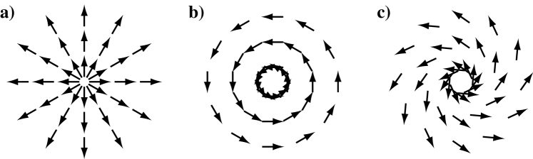
Figure 1: Schematic representation of the geometry of point defects of topological charge one in two dimensions. Displayed are the orientations of polarization vectors as arrows for (a) aster, (b) vortex and (c) spiral.

For $\Delta\mu=0$, the system reaches an equilibrium steady state where all fluxes and forces vanish: $\sigma_{\alpha\beta}=0$, $u_{\alpha\beta}=0$, $P_{\alpha}=0$, $h_{\alpha}=0$ and $r=0$. The equilibrium orientation of the polarization ${\bf p}$, corresponds to a vanishing orientational field $h_{\alpha}=-\delta F/\delta p_{\alpha}=0$. In order to describe point defects, it is convenient to introduce polar coordinates $(r,\theta)$ and the angle $\psi(r,\theta)$ which characterizes the components of the vector ${\bf p}$: $(p_{r}=\cos\psi$, $p_{\theta}=\sin\psi)$, see Fig. 1(a). The components of the orientational field $h_{\alpha}$ in cylindrical coordinates can be written as $h_{r}=h_{\|}\cos\psi-h_{\perp}\sin\psi$, and $h_{\theta}=h_{\|}\sin\psi+h_{\perp}\cos\psi$, where we have introduced the components $h_{||}$ and $h_{\perp}$ parallel and perpendicular to the direction of ${\bf p}$.

Considering for simplicity rotationally symmetric fields describing point defects with $\psi=\psi(r)$, we obtain

$$F = 2\pi\int dr\;r\left\{\frac{K}{2}\left(\frac{1}{r}\frac{d}{dr}r\cos\psi\right)^{2}\right.$$ (47)

$$+ \left.\frac{K+\delta K}{2}\left(\frac{1}{r}\frac{d}{dr}r\sin\psi\right)^{2}\right\}\quad.$$

where we have ignored the spontaneous splay which leads to a boundary term.

The perpendicular field is obtained by taking the functional derivative of the free energy $h_{\perp}=-\delta F/\delta\psi$

$$h_{\perp} = (K+\delta K\cos^{2}\psi)\left[\psi^{\prime\prime}+\frac{\psi^{\prime}}{r}\right]$$ (48)

$$- \frac{\delta K}{2}\sin 2\psi\left[\frac{1}{r^{2}}+\psi^{\prime 2}\right]$$

where the prime indicates derivation with respect to $r$. The value of the Lagrange multiplier $h_{\|}$ (the longitudinal field) is chosen in such a way that the condition ${\bf p}^{2}=1$ is satisfied.

Four types of topological defects of charge one are possible, see Fig. 1(a) and (b). If we assume that boundary conditions are always chosen to allow for solutions with constant $\psi$, these solutions corresponds to asters with $\psi(r)=0$ and $\psi(r)=\pi$ and to vortices with $\psi(r)=\pm\pi/2$. The linear stability of asters and vortices against angular perturbations $\delta\psi(r)$ is described by

$$\frac{\gamma_{1}}{1+\gamma_{1}(\nu_{1}\pm 1)^{2}/(4\eta)}\frac{\partial\delta\psi}{\partial t} =$$

$$(K+\delta K\cos^{2}\psi ) \left(\frac{d^{2}}{dr^{2}}+\frac{1}{r}\frac{d}{dr}\right)\delta\psi$$

$$- \delta K \cos(2\psi)\frac{1}{r^{2}}\delta\psi(r)$$ (49)

where the minus sign corresponds to an aster and teh plus sign to a vortex. If all the eigenvalues of the linear operator on the right hand side are negative, the defect is stable, and otherwise it is unstable. (We may note that this operator has the form of the negative a quantum Hamiltonian of one particle.) Asters are stable for positive $\delta K$ while vortices are stable for $\delta K$ negative. For the special case $\delta K=0$, Eq. (V.1) becomes $\gamma_{1}\partial\psi/\partial t=K\Delta\psi$, where $\Delta$ denotes the Laplace operator, and defects for any value $\psi(r)=\psi_{0}$ are stable. These defects are called spirals since the direction of polarization follows spirals with an equation in polar coordinates given by

$$r(\theta)=r_{0}\exp[\cot(\psi_{0})\theta]\quad,$$ (50)

see Fig 1. (c).

V.2 Non-equilibrium steady states

We now discuss the effect of a point defect in two dimensions if motors in the system are active and $\Delta\mu\neq 0$. In this situation, spiral defects start to rotate and there are nontrivial flow and stress profiles. We assume that the system is incompressible, i.e., $u_{rr}+u_{\theta\theta}=0$. Using the expression of the strain rate tensor given in appendix, this imposes that $v_{r}=\alpha/r$. The absence of singularity of the radial velocity for small $r$ implies that $\alpha=0$, therefore $v_{r}=0$ and $u_{rr}=u_{\theta\theta}=0$.

The Onsager Eq. (28) for the polarization rate can then be written in cylindrical coordinates. In a steady state, $P_{\alpha}=0$, we obtain at linear order:

$$\nu_{1}u_{r\theta}\sin 2\psi = \frac{h_{\|}}{\gamma_{1}}+\lambda_{1}\Delta\mu$$ (51)

$$(\nu_{1}\cos 2\psi-1)u_{r\theta} = \frac{h_{\perp}}{\gamma_{1}}\quad.$$ (52)

where we have expressed the orientational field $h_{\alpha}$ in terms of its parallel and perpendicular coordinates. Similarly, Eqns. (27)-(29) can be rewritten in polar coordinates. Using $u_{rr}=u_{\theta\theta}=0$ and only taking terms to linear order in the generalized forces into account we find that the steady state obeys

$$0 = \sigma_{rr}+\zeta\Delta\mu\cos^{2}\psi+(\bar{\zeta}+\zeta^{\prime})\Delta\mu$$ (53)

$$-\nu_{1}\left[h_{\|}\cos^{2}\psi-\frac{1}{2}h_{\perp}\sin 2\psi\right]$$

$$-\bar{\nu}_{1}h_{\|}$$

$$0 = \sigma_{\theta\theta}+\zeta\Delta\mu\sin^{2}\psi+(\bar{\zeta}+\zeta^{\prime})\Delta\mu$$ (54)

$$-\nu_{1}\left[h_{\|}\sin^{2}\psi+\frac{1}{2}h_{\perp}\sin 2\psi\right]$$

$$-\bar{\nu}_{1}h_{\|}$$

$$2\eta u_{r\theta} = \sigma_{r\theta}+\frac{\zeta}{2}\Delta\mu\sin 2\psi$$ (55)

$$-\frac{1}{2}\nu_{1}\left[h_{\|}\sin 2\psi+h_{\perp}\cos 2\psi\right]\quad.$$

In addition to the dynamic equations Eqns. (27)-(29), the force balance Eq. (4) has to be satisfied. The $\theta$ component of the force balance equation ( Eq. (78) of appendix A) is solved by $\sigma^{\rm tot}_{r\theta}=B/r^{2}$ where $B$ is an integration constant. Since $\sigma^{\rm tot}_{r\theta}$ must not diverge, $B=0$ and therefore $\sigma^{\rm tot}_{r\theta}=0$ and $\sigma_{r\theta}=h_{\perp}/2$. The components $\sigma_{rr}$ and $\sigma_{\theta\theta}$ of the stress tensor follow from Eqns. (53) and (54). These stresses together with the radial component of the force balance equation (Eq. (77) of appendix A) determine the pressure profile $\Pi$ required to ensure the incompressibility of the material.

V.3 Asters, vortices and spirals

We now determine the stationary solutions for point defects in non-equilibrium states. From Eq. (51) we find an expression for the parallel component of the orientational field

$$h_{\|}=\gamma_{1}(\nu_{1}u_{r\theta}\sin 2\psi-\lambda_{1}\Delta\mu)\quad.$$ (56)

Inserting this expression in Eq. (55), we obtain the non diagonal strain rate

$$u_{r\theta}=\frac{\tilde{\zeta}\Delta\mu\sin 2\psi+h_{\perp}(1-\nu_{1}\cos 2\psi)}{4\eta+\gamma_{1}\nu_{1}^{2}\sin^{2}2\psi}$$ (57)

where $\tilde{\zeta}=\zeta+\nu_{1}\gamma_{1}\lambda_{1}$. This equation together with Eq. (52), where $h_{\perp}$ is given by Eq. (48) determines $\psi$ and $u_{r\theta}$. Eliminating $u_{r\theta}$, we find an equation for the steady state orientation $\psi$

$$h_{\perp}(4\eta+\gamma_{1}(\nu_{1}^{2}+1-2\nu_{1}\cos 2\psi))=\gamma_{1}\sin 2\psi(\nu_{1}\cos 2\psi-1)\tilde{\zeta}\Delta\mu$$ (58)

We now discuss special solutions to this equations as well as the stability of asters and vortices obtained at thermal equilibrium for $\Delta\mu=0$.

V.3.1 Spiral solutions for $\delta K=0$

We first consider the simple case where there is no anisotropy of the elastic constants: $\delta K=0$ and $h_{\perp}=K\Delta\psi$. Eq. (52) requires that spirals with constant $\psi_{0}$ and $h_{\perp}=0$ satisfy $\cos 2\psi_{0}=1/\nu_{1}$. This selection of angle, which depends on the parameter $\nu_{1}$ is a dynamic phenomenon. The same angle is selected for the orientation of nematic liquid crystals in shear flows. A steady state exists only if $|\nu_{1}|\geq 1$. The polarization angle takes one of the two values

$$\psi_{0}=\pm\frac{1}{2}\arccos\frac{1}{\nu_{1}}$$ (59)

in the interval $[-\pi,\pi]$. With these values of $\psi_{0}$, we find

$$u_{r\theta}=\frac{\sin 2\psi_{0}}{4\eta+\gamma_{1}\nu_{1}^{2}\sin^{2}2\psi_{0}}\tilde{\zeta}\Delta\mu\quad.$$ (60)

The velocity is ortho-radial, along the $\theta$ direction; it is obtained from (75)

$$v_{\theta} = 2r\left(\int_{0}^{r}\frac{u_{r\theta}}{r^{\prime}}dr^{\prime}+v_{\theta}^{0}\right)$$ (61)

where $v_{\theta}^{0}$ is an integration constant. For a finite system with radius $R$ and with the boundary condition that no motion occurs at the boundary,

$$v_{\theta}=2u_{r\theta}r\log\frac{r}{R}\quad.$$ (62)

V.3.2 Stability of asters and vortices

Both asters with $\psi_{0}=0,\pi$ and vortices $\psi_{0}=\pm\pi/2$ are solutions to Eq.(58). In order to understand under which conditions these solutions are stable, we perform a linear stability analysis, writing $\psi(r)=\psi_{0}+\delta\psi$. The time-dependence of $\psi$ in the liquid limit $\tau\rightarrow 0$ is given by

$$\gamma_{1}\frac{\partial\psi}{\partial t}=h_{\perp}-\gamma_{1}(\nu_{1}\cos 2\psi-1)u_{r\theta}$$ (63)

Linearizing this equation and using Eq. (57) we find for asters with $\psi_{0}=0$ and $\delta K>0$ that $\delta\psi(r)$ satisfies to linear order

$$\frac{\gamma_{1}}{1+\gamma_{1}(\nu_{1}-1)^{2}/(4\eta)}\frac{\partial}{\partial t}\delta\psi={\cal L}\delta\psi$$ (64)

where the linear operator is given by

$${\cal L}=(K+\delta K)\left(\frac{d^{2}}{dr^{2}}+\frac{1}{r}\frac{d}{dr}-\frac{n^{2}}{r^{2}}+k^{2}\right),$$ (65)

Here, we have defined $n^{2}=\delta K/(K+\delta K)$ and $k^{2}=-\frac{2\tilde{\zeta}\Delta\mu(\nu_{1}-1)\gamma_{1}}{[4\eta+\gamma_{1}(\nu_{1}-1)^{2}](K+\delta K)}$. An aster solution becomes unstable, if the largest eigenvalue of ${\cal L}$ vanishes. The condition ${\cal L}\delta\psi=0$ is solved by Bessel functions of order $n$, $\delta\psi\sim J_{n}(kr)$. For a finite system with radius $R$ we find with boundary conditions $\delta\psi(R)=0$ that $kR=z_{n}$, where $z_{n}$ denotes the first positive root of $J_{n}(z)$. Therefore, the critical value for the instability of asters is given by

$$\tilde{\zeta}\Delta\mu_{c}^{A}=-\left(\frac{z_{n}}{R}\right)^{2}\frac{4\eta+\gamma_{1}(\nu_{1}-1)^{2}}{2\gamma_{1}(\nu_{1}-1)}(K+\delta K)$$ (66)

In the case of vortices with $\psi_{0}=\pm\pi/2$ and $\delta K<0$, we find

$$\frac{\gamma_{1}}{1+\gamma_{1}(\nu_{1}+1)^{2}/(4\eta)}\frac{\partial\delta\psi}{\partial t}={\cal L}^{\prime}\delta\psi$$

$${\cal L}^{\prime}=K\left(\frac{d^{2}}{dr^{2}}+\frac{1}{r}\frac{d}{dr}-\frac{m^{2}}{r^{2}}+q^{2}\right),$$ (67)

where $m^{2}=-\delta K/K$ and $q^{2}=-\frac{2\tilde{\zeta}\Delta\mu(\nu_{1}+1)\gamma_{1}}{[4\eta+\gamma_{1}(\nu_{1}+1)^{2}]K}$. Following the same analysis as for asters, the instability of vortices occurs for

$$\tilde{\zeta}\Delta\mu_{c}^{V}=-\left(\frac{z_{m}}{R}\right)^{2}\frac{4\eta+\gamma_{1}(\nu_{1}+1)^{2}}{2\gamma_{1}(\nu_{1}+1)}K$$ (68)

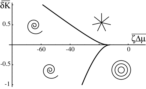
Figure 2: Stability diagram of asters, vortices and spirals which are topological defects in an active gel of polar filaments. Asters are stable for $\delta K>0$ in the region with actively generated stresses $\tilde{\zeta}\Delta\mu$ larger than a critical value $\tilde{\zeta}\Delta\mu^{A}_{c}$. This critical value is negative, corresponding to contractile stresses in the gel. Vortices are stable for $\delta K<0$ and $\tilde{\zeta}\Delta\mu>\tilde{\zeta}\Delta\mu^{V}_{c}$. For other parameter values, rotating spirals occur via a symmetry breaking dynamic instability. Here, $\overline{\delta K}=\delta K/K$ is a dimensionless ratio of two elastic moduli and $\overline{\zeta\Delta\mu}=R^{2}\tilde{\zeta}\Delta\mu/K$ a dimensionless measure of active stresses. Note that both rotation senses occur with equal probability on symmetry grounds. The diagram was evaluated for the choice $\eta/\gamma_{1}=1$ and $\nu_{1}=2$ of Onsager coefficients of the system.

The resulting stability diagram in the $(\tilde{\zeta}\Delta\mu,\delta K)$-plane is displayed on Fig. 2. We have assumed on this diagram that $\nu_{1}\geq 1$. There are three regions on this diagram, a region with positive $\delta K$ and positive $\tilde{\zeta}\Delta\mu$ where the asters are stable, a region with negative $\delta K$ and positive $\tilde{\zeta}\Delta\mu$ where vortices are stable and a region with large negative $\tilde{\zeta}\Delta\mu$ where spiral defects are stable. Along the line $\delta K=0$, spirals are always stable as studied in the previous paragraph. We do not give here a general description of the spiral defects, as in the case where $\delta K=0$, we expect that there is a dynamic selection of the orientational angle and that the defect is rotating.

V.4 Effects of friction with the substrate

So far we have considered the point defect in a real two-dimensional space. A real active gel interacts with both the surrounding solvent and the substrate. We do not discuss the hydrodynamic interactions between the gel and the solvent here. We now consider a thin quasi-two dimensional gel layer and introduce a friction force at the substrate proportional to the local velocity. Taking into account the rotational symmetry, the friction force modifies the ortho-radial ($\theta$) component of the force balance that becomes

$$\frac{\partial\sigma_{r\theta}}{\partial r}+\frac{2}{r}\sigma_{r\theta}=\xi v_{\theta},$$ (69)

This equation, which is a balance between the friction force and the tangential stress can be integrated for a rotating spiral defect, yielding the following expression for the tangential stress as a function of the velocity.

$$\sigma_{r\theta}=\frac{\xi}{r^{2}}\int_{0}^{r}dr^{\prime}\;r^{\prime 2}v_{\theta}(r^{\prime})$$ (70)

In the absence of elastic constant anisotropy, $\delta K=0$, we can derive the velocity profile $v_{\theta}(r)$ in an infinite system from Eq. (70) as follows: We look for a solution of Eq. (52) with $h_{\perp}=0$ and $\psi=$const.. As in the absence of friction, the polarization angle can have one of the 4 possible values satisfying $\cos 2\psi_{0}=1/\nu_{1}$. The velocity field is then obtained from Eq. (55) that can be transformed into the following ordinary differential equation for $v_{\theta}$:

$$\frac{d}{dz}z^{3}\left(-\frac{v_{\theta}}{z^{2}}+\frac{1}{z}\frac{dv_{\theta}}{dz}\right)=z^{2}v_{\theta}+2\lambda_{f}\omega_{0}z,$$ (71)

where $z=r/\lambda_{f}$ and the the friction length is given by ${\lambda_{f}=(4\eta+\gamma_{1}\nu_{1}\sin^{2}2\psi_{0})^{1/2}/(2\xi^{1/2})}$. The velocity is then given by

$$v_{\theta}(r)=2\omega_{0}\lambda_{f}\left\{K_{1}(\frac{r}{\lambda_{f}})-\frac{\lambda_{f}}{r}\right\},$$ (72)

where $K_{1}$ is the modified Bessel function of the second kind defined in Ref. abra72 ,

At short distances ($r\ll\lambda_{f}$), the dissipation is dominated by the viscosity $\eta$ and the velocity field is the same as in the absence of friction. At large distances, the dissipation is dominated by the friction on the substrate $\xi$ and the velocity $v_{\theta}$ decays to zero. The stability diagram of the defect in the presence of substrate friction is very similar to the diagram of Fig. (3) where the finite size $R$ would be replaced by the friction length $\lambda_{f}$.

VI Discussion

We have introduced in this manuscript equations which describe the long wavelength and low frequency behavior of active gels. Although we have written the equations specifically in the case where the activity is due to motor proteins, they should apply, in their principles, to all gels in which a permanent source of dissipation is at work. Such gels define a new class of materials. For instance, a conventional ”physical” polar gel, absorbing a high frequency ultrasonic wave should obey, in the low frequency, long wavelength limit, the set of equations proposed here. Our main motivation however, is the construction of a generic theory for characterizing quantitatively the properties of Eukaryotic biological gels. One could object that generalized hydrodynamic theories involve a large number of parameters and are thus not very useful. Their merit is to involve the smallest number of parameters required for a relevant description of the systems under consideration and to describe in a unified way all long length scale and long time scale situations which are otherwise seemingly unconnected. The nature of most parameters is already well-known for gel or polymer rheology or for liquid crystal physics, and their measurement techniques can straightforwardly be transfered to active gels. This is transparent for translational, orientational elastic moduli and viscosities. Coefficients linking shear flow and polar orientation are less familiar to the general public but are well known to liquid crystal physicists, and their measurements are not difficult a priori. There are six bulk and two surface additional parameters, compared to a passive polar gel. Among the bulk quantities one is equivalent to the motor velocity on the actin filaments ($\lambda)$, and another one is the depolymerization rate $k_{d}$ of the gel in the bulk. Both quantities are directly accessible to experiment. Surface polymerization terms can be extracted independently from biochemical data and although they generate a new interesting physics (howa01 ; pros01 ), they do not introduce uncertainties in the description.

Among the four remaining parameters, three ($\zeta$, $\bar{\zeta}$ and $\zeta^{\prime}$ bear essentially the same physics (i.e: the activity implies either spontaneous motion or spontaneous stress), and the last one $\lambda_{1}$ measures the active rate of change of polarization. Hence, there are only two relevant additional parameter, namely $\lambda_{1}$ and $\zeta$ with respect to a passive polar gel. We show, in the two examples developed here, that they change profoundly the behavior of gels: behaviors which in the absence of energy input would be static, become dynamic. The structure of the relaxation modes which would be entirely over-damped in the long wavelength limit, now can support propagative waves rama00 ; simh02 , spiral disclinations rotate permanently. Many other consequences have to be unraveled. Knowing that it has taken more than ten years to investigate the properties of generalized hydrodynamical equations relevant to liquid crystals, it is likely that a similar number of years will be necessary in this case as well. Our bet is that it will help us understand the complex behavior of the slow dynamics of the eukaryotic cytoskeleton in a robust way, not depending on the details of the involved proteins.

Our theory can be extended in several ways. First we have ignored the permeation process of the bulk fluid through the gel. This is legitimate in the long time limit in most geometries but not all. The inclusion of permeation in our equations would be straightforward. We have also used the simplest visco-elastic gel theory: experiments performed on cells suggest the existence of scale invariant visco-elastic behavior which could also be included in the theory fabr01 . At last we have assumed that the driving force was ”small” and constant both in space and time. The spatial and temporal invariance make sense in a cell since the $ATP$ production centers seem to be abundant and evenly distributed. In vitro experiments may mimic these conditions on a limited time scale, yet large compared to most phenomena of interest. Furthermore there is no a priori difficulty in introducing $ATP$ production and consumption in the equations. More severe is the last limitation: our equations are valid for $\Delta\mu$ small compared to thermal energy, whereas it is of the order of ten time that value in real life. The extension of our theory to large $\Delta\mu$ is a real challenge and will probably require some feedback from experiments. A brute force expansion in higher powers of forces and fluxes is just totally impractical and would leave out the known and probably leading exponential dependences of polymerization/depolymerization rates on stress. Other challenging questions concern the nature of noise which will pick up strong out of equilibrium contributions, and possible dynamical transitions for instance in the motor behaviorjuli97 . For these reasons, we think that is it wise to start with the well controlled approach that we propose here and to develop the corresponding experiments. This will help us familiarize with this new physics before getting to regions of phase space were we lack guiding principles.

An important application of active gels is the problem of cell locomotion on a substrate sperm . In a forthcoming publication, we will discuss how the interplay of polymerization and activity can induce the motion of a thin layer of an active gel on a solid surface. The physics of this gel motion coupled to the properties of bio-adhesion provides a basis for an understanding of the locomotion of cells such as keratocytes verk98 .

Appendix A Cylindrical coordinates

In polar coordinates, the rate of strain tensor for a rotationally symmetric velocity profile is given by

$$u_{rr} = \frac{d}{dr}v_{r}$$ (73)

$$u_{\theta\theta} = \frac{v_{r}}{r}$$ (74)

$$u_{r\theta} = \frac{r}{2}\frac{d}{dr}\left(\frac{v_{\theta}}{r}\right)\quad.$$ (75)

Furthermore,

$$\omega_{r\theta}=\frac{1}{2r}\frac{d}{dr}(rv_{\theta})\quad.$$ (76)

If the system is invariant by rotation, the local force balance in cylindrical coordinates is written as

$$\frac{1}{r}\frac{d}{dr}\left(r\sigma^{\rm tot}_{rr}\right)-\frac{1}{r}\sigma^{\rm tot}_{\theta\theta} = \frac{d\Pi}{dr}$$ (77)

$$\frac{1}{r^{2}}\frac{d}{dr}\left(r^{2}\sigma^{\rm tot}_{r\theta}\right) = 0\quad,$$ (78)

In an incompressible system, the pressure $\Pi$ is a Lagrange multiplier necessary to impose the incompressibility constraint.

Appendix B Viscoelastic polar gel

The form of Equations (17), (18), (23) and (25) can be understood by discussing the general dynamics of the polarization field $p_{\alpha}$ in frequency space. As a function of frequency, we write to linear order

$$i\omega\tilde{p}_{\alpha}=\frac{\tilde{h}_{\alpha}}{\gamma_{1}}+\lambda_{1}\tilde{p}_{\alpha}\Delta\mu-\frac{1}{1+i\omega\tau}(\nu_{1}p_{\beta}\tilde{u}_{\alpha\beta}+\bar{\nu}_{1}p_{\alpha}\tilde{u}_{\beta\beta})...$$ (79)

where the tilde denotes a Fourier amplitude at frequency $\omega$. The first two terms of the right hand side correspond to a straightforward linear response theory of a ferroelectric liquid crystal. Similarly, the last term provides for $\omega=0$ the reactive linear coupling term allowed by symmetry. For finite frequency furthermore, this term takes into account that the gel is elastic on short time scales or large $\omega$. This can be seen as follows: in the case of an elastic gel, the free energy $F$ of the polarization field contains elastic terms of the form

$$F_{\rm el}=\frac{\gamma_{1}\nu_{1}}{2\tau}\int d^{d}xp_{\alpha}\epsilon_{\alpha\beta}p_{\beta}$$ (80)

where $\epsilon_{\alpha\beta}$ is the strain tensor characterizing deformations of the gel. This leads to a modification of $h_{\alpha}$ by $h_{\alpha}^{\rm el}=-\delta F_{\rm el}/\delta p_{\alpha}$. Since in frequency space, $\tilde{u}_{\alpha\beta}=i\omega\tilde{\epsilon}_{\alpha\beta}$, Eq. (79) does describe the correct elastic limit for large $\omega$ Separating Eq. (79) in reactive and dissipative parts, using the opposite signatures with respect to time reversal (or equivalently $\omega\rightarrow-\omega$) allows us to identify $P_{\alpha}^{d}$ and $P_{\alpha}^{r}$. Using $1/(1+i\omega\tau)=1-i\omega\tau/(1+\omega^{2}\tau^{2})$ and replacing $i\omega$ by $D/Dt$, we can write the reactive and dissipative parts of $P_{\alpha}$ as given by Eqns. (18)and (25). Symmetry relations now impose the correct equations for $\sigma^{d}_{\alpha\beta}$ and $\sigma^{r}_{\alpha\beta}$ as given by Eqns. (17) and (23).

References

- (1) B. Alberts et al., Molecular Biology of the Cell 4th ed. (Garland, New York, 2002).
- (2) D. Bray, Cell Movements 2nd ed. (Garland, New York, 2001).
- (3) J. Howard, Mechanics of Motor Proteins and the Cytoskeleton (Sinauer Associates, Inc., Sunderland, 2001).
- (4) R. Lipowsky and E. Sackmann, editors, Structure and dynamics of membranes - from cells to vesicles, Vol. 1 of Handbook of biological physics (Elsevier, Amsterdam, 1995).
- (5) J.-B. Manneville, P. Bassereau, S. Ramaswamy, J. Prost, Phys. Rev. E 64, 021908 (2001).
- (6) D.A. Head, A.J. Levine, F.C. MacKintosh, Phys. Rev. Lett. 91, 108102 (2003).
- (7) J. Wilhelm and E, Frey, Phys. Rev. Lett. 91, 108103 (2003).
- (8) K.Takiguchi J.Biochem. 109, 520 (1991).
- (9) F.J. Nédélec et al., Nature 389, 305 (1997).
- (10) T. Surrey et al., Proc. Natl. Acad. Sci. USA 95, 4293 (1998).
- (11) F.J. Nédélec, T. Surrey, and A.C. Maggs, Phys. Rev. Lett. 86, 3192 (2001).
- (12) T. Surrey et al., Science 292, 1167 (2001).
- (13) K. Sekimoto and H. Nakazawa, in Current topics in physics, Y.M. Choe, J.B. Hong and C.N. Chang (eds.), p. 394 (World scientific, Singapore 1998), physics/0004044.
- (14) K. Kruse and F. Jülicher, Phys. Rev. Lett. 85, 1778 (2000).
- (15) K. Kruse, S. Camalet, and F. Jülicher, Phys. Rev. Lett. 87, 138101 (2001).
- (16) K. Kruse and F. Jülicher, Phys. Rev. E 67, 051913 (2003).
- (17) K. Kruse, A. Zumdieck and F. Jülicher, Europhys. Lett. 64, 716 (2003).
- (18) H.Y. Lee and M. Kardar, Phys. Rev. E 64, 056113 (2001).
- (19) J. Kim et al., J. Korean Phys. Soc. 42, 162 (2003).
- (20) T.B. Liverpool and M.C. Marchetti, Phys. Rev. Lett. 90, 138102 (2003).
- (21) P.C.Martin, O.Parodi and P.Pershan, Phys. Rev. A 6, 2401 (1972).
- (22) P.G. DeGennes, Scaling concepts in polymer physics Cornell University Press, Ithaca (1985).
- (23) K.Sekimoto J:Phys.II (France) 1, 19 (1991).
- (24) A. Simha and S. Ramaswamy, Phys. Rev. Lett. 89, 058101 (2002).
- (25) K. Kruse, J.F. Joanny, F. Jülicher, J. Prost and K. Sekimoto, Phys. Rev. Lett 92, 078101 (2004).
- (26) R.B. Bird et al. Dynamics of Polymeric Liquids 2nd ed. (Wiley, New York, 1987).
- (27) R. Larson, Constitutive Equations for Polymer Melts and Solutions (Butterworth-Heinemann, 1998).
- (28) M.G.Vicker, Exp. Cell Res. 27554 (2002).
- (29) T. Bretschneider et al., Curr. Biol.14, 1 (2004).
- (30) G. Giannone et al. Cell 116, 431 (2004).
- (31) S. Ramaswamy, J. Toner, J. Prost, Phys. Rev. Lett. 84, 3494 (2000).
- (32) P.G. De Gennes and J. Prost, The Physics of Liquid Crystals (Clarendon Press, Oxford 1993).
- (33) M. Abramowitz and I.A. Stegun (eds.), Handbook of Mathematical Functions (Dover, 1972).
- (34) J. Prost in Physics of bio-molecules and cells, Flyvbjerg, H., Jülicher, F., Ormos, P., David, F., Eds. (EDP Sciences, Les Ulis, 2001), 215-236.
- (35) B. Fabry, G.N. Maksym, J.P. Butler, M. Glogauer, D. Navajas, J. Fredberg, Phys. Rev. Lett.87, 148102 (2001).
- (36) F. Jülicher, A. Ajdari, J. Prost, Rev. Mod. Phys. 69 1269 (1997).
- (37) J.F.Joanny, F.Jülicher and J.Prost, Phys. Rev. Lett. 90, 168102 (2003).
- (38) A.Verkhovsky, T. Svitkina and G.Borisy, Current Biology 9, 11 (1998). A.B. Verkhovsky, T.M. Svitkina and G.G. Borisy, Curr. Biol 9, 11 (1999).