An Exact Formula to Describe the Amplification Process in a Photomultiplier Tube

Abstract

An analytical function is derived that exactly describes the amplification process due to a series of discrete, Poisson-like amplifications like those in a photo multiplier tube (PMT). A numerical recipe is provided that implements this function as a computer program. It is shown how the program can be used as the core-element of a faster, simplified routine to fit PMT spectra with high efficiency. The functionality of the method is demonstrated by fitting both, Monte Carlo generated and measured PMT spectra.

1 Introduction

In September 1999, the LHCb RICH group tested Hamamatsu’s 64-Multi-anode Photo Multiplier Tubes as a possible photodetector choice for the LHCb RICH detector [RIC00]. During the data analysis, the need for an accurate model of the output of a PMT arose that could be fitted to the measured pulse height spectra, mainly in order to have a precise estimate of the signal lost below the threshold cut. In order to perform a fit to the spectra, an analytical function is needed that can be calculated reasonably quickly by a computer.

Such a function is derived here. First (section 2), an analytical expression is derived that describes the output of a PMT. The starting assumption is that the number of photoelectrons per event, as well as the number of secondary electrons caused by each primary electron at each stage of the dynode chain, are well described by Poisson distributions. Furthermore it is shown how this expression can be adapted to avoid some of the numerical problems arising in the original expression, so that it can be calculated by a computer. A complete numerical recipe is given and a FORTRAN implementation of the program is listed in appendix A. This expression can of course be used to calculate any “snowball” like effect described by a series of Poisson distributions.

In section 3 it is described how the exact expression derived in the first part can be used as the central element of a faster, approximate function, and how the number of parameters can be reduced making reasonable assumptions, so that fitting a large number of spectra in a finite time becomes feasible. This is then adapted to describe the digitised output of laboratory read-out electronics, rather than the number of electrons at the end of a dynode chain.

This approximate function is used in section 4 of the paper to fit Monte Carlo generated spectra as well as real data, demonstrating the validity of the method.

2 An Analytical Function

2.1 The Electron Probability Distribution

In the following, an expression for the number of photoelectrons at the end of a dynode chain of a PMT is derived. The number of incident photons, and hence of photoelectrons produced in the cathode, is assumed to follow a Poisson distribution. This is appropriate for the testbeam data where PMTs were used to detect Cherenkov photons generated by a particle traversing a dielectric. With a mean number of photoelectrons produced in the cathode of $\lambda_{1}$, the probability to find $k_{1}$ photoelectrons arriving at the first dynode is:

$$P(k_{1})=e^{-\lambda_{1}}\frac{\lambda_{1}^{k_{1}}}{k_{1}!}.$$ (1)

The probability to find $k_{2}$ electrons after the first dynode is the sum over all values for $k_{1}$ of the probabilities $P(k_{1})$, each multiplied by the probability that the dynode returns $k_{2}$ electrons given that $k_{1}$ arrive:

$$P(k_{2})=\sum_{k_{1}=0}^{\infty}P(k_{1})\cdot P(k_{2}|k_{1}).$$ (2)

Each of the $k_{1}$ electrons produces a Poisson–distributed response from the dynode with mean $\lambda_{2}$ where $\lambda_{2}$ is the gain at the $1^{\mathrm{st}}$ dynode; all $k_{1}$ electrons together produce a response distributed according to the convolution of $k_{1}$ Poisson distributions, each with mean $\lambda_{2}$. This results in a single Poisson distribution with mean $\lambda_{2}\cdot k_{1}$:

$$P(k_{2}|k_{1})=e^{-\lambda_{2}k_{1}}\frac{\left(\lambda_{2}k_{1}\right)^{k_{2}}}{k_{2}!}.$$ (3)

Hence the probability to find $k_{2}$ electrons after the first dynode is given by:

$$P(k_{2})=\sum_{k_{1}=0}^{\infty}P(k_{1})\cdot e^{-\lambda_{2}k_{1}}\frac{\left(\lambda_{2}k_{1}\right)^{k_{2}}}{k_{2}!}.$$ (4)

Inserting the right–hand side of equation 1 for $P(k_{1})$ yields, after manipulation:

$$P(k_{2})=e^{-\lambda_{1}}\frac{\lambda_{2}^{k_{2}}}{k_{2}!}\sum_{k_{1}=0}^{\infty}\frac{(\lambda_{1}e^{-\lambda_{2}})^{k_{1}}}{k_{1}!}k_{1}^{k_{2}}.$$ (5)

Generalising this for $n-1$ dynodes yields:
$\displaystyle P(k_{n})$ $\displaystyle=$ $\displaystyle e^{-\lambda_{1}}\frac{\lambda_{n}^{k_{n}}}{k_{n}!}$ $\displaystyle\sum_{k_{1}=0}^{\infty}\sum_{k_{2}=0}^{\infty}\cdots\sum_{k_{n-1}=0}^{\infty}$ $\displaystyle\frac{(\lambda_{1}e^{-\lambda_{2}})^{k_{1}}}{k_{1}!}\frac{(\lambda_{2}e^{-\lambda_{3}}k_{1})^{k_{2}}}{k_{2}!}$ $\displaystyle\frac{(\lambda_{3}e^{-\lambda_{4}}k_{2})^{k_{3}}}{k_{3}!}\cdots$ $\displaystyle\frac{(\lambda_{n-2}e^{-\lambda_{n-1}}k_{n-3})^{k_{n-2}}}{k_{n-2}!}$ $\displaystyle\frac{(\lambda_{n-1}e^{-\lambda_{n}}k_{n-2})^{k_{n-1}}}{k_{n-1}!}k_{n-1}^{k_{n}}.$
Each term in equation 2.1 is of the form of an exponential series, i.e. $\frac{x^{k}}{k!}$, except for the last term with the summation parameter $k_{n-1}$, which appears as $\frac{x^{k}}{k!}k^{k_{n}}$. This term can be expressed in terms of the $k_{n}$th derivative of $e^{yk_{n-1}}$ with respect to the new variable $y$ at $y=0$:

$$k_{n-1}^{k_{n}}=\frac{\mathsf{d}^{k_{n}}}{\mathsf{d}y^{k_{n}}}e^{yk_{n-1}}\Big{|}_{y=0}.$$ (7)

Now the last term in equation 2.1 can be written as
$\displaystyle\frac{(\lambda_{n-1}e^{-\lambda_{n}}k_{n-2})^{k_{n-1}}}{k_{n-1}!}k_{n-1}^{k_{n}}$ (8) $\displaystyle=$ $\displaystyle\frac{\mathsf{d}^{k_{n}}}{\mathsf{d}y^{k_{n}}}\frac{(\lambda_{n-1}e^{-\lambda_{n}}k_{n-2}e^{y})^{k_{n-1}}}{k_{n-1}!}\bigg{|}_{y=0}.$
Using 8, equation 2.1 can be re–written as: $\displaystyle P(k_{n})$ $\displaystyle=$ $\displaystyle e^{-\lambda_{1}}\frac{\lambda_{n}^{k_{n}}}{k_{n}!}\;\;\;\;\;\frac{\mathsf{d}^{k_{n}}}{\mathsf{d}y^{k_{n}}}$ $\displaystyle\sum_{k_{1}=0}^{\infty}\sum_{k_{2}=0}^{\infty}\cdots\sum_{k_{n-1}=0}^{\infty}$ $\displaystyle\frac{(\lambda_{1}e^{-\lambda_{2}})^{k_{1}}}{k_{1}!}\frac{(\lambda_{2}e^{-\lambda_{3}}k_{1})^{k_{2}}}{k_{2}!}$ $\displaystyle\frac{(\lambda_{3}e^{-\lambda_{4}}k_{2})^{k_{3}}}{k_{3}!}\cdots$ $\displaystyle\frac{(\lambda_{n-2}e^{-\lambda_{n-1}}k_{n-3})^{k_{n-2}}}{k_{n-2}!}$ $\displaystyle\frac{(\lambda_{n-1}e^{-\lambda_{n}}k_{n-2}e^{y})^{k_{n-1}}}{k_{n-1}!}\bigg{|}_{y=0}.$
Now each summation can be carried out in turn, starting with that over $k_{n-1}$:

$$\sum_{k_{n-1}=0}^{\infty}\frac{(\lambda_{n-1}e^{-\lambda_{n}}k_{n-2}e^{y})^{k_{n-1}}}{k_{n-1}!}$$

$$= \exp(\lambda_{n-1}e^{-\lambda_{n}}k_{n-2}e^{y})$$

$$= (\exp(\lambda_{n-1}e^{-\lambda_{n}}e^{y}))^{k_{n-2}},$$

then over $k_{n-2}$:

$$\sum_{k_{n-2}=0}^{\infty}\Big{(}\frac{(\lambda_{n-2}e^{-\lambda_{n-1}}k_{n-3})^{k_{n-2}}}{k_{n-2}!}\cdot$$

$$(e^{(\lambda_{n-1}e^{-\lambda_{n}}e^{y})})^{k_{n-2}}\Big{)}$$

$$= \exp(\lambda_{n-2}e^{-\lambda_{n-1}}k_{n-3}\cdot e^{(\lambda_{n-1}e^{-\lambda_{n}}e^{y})})$$

$$= (\exp(\lambda_{n-2}e^{-\lambda_{n-1}}\cdot e^{(\lambda_{n-1}e^{-\lambda_{n}}e^{y})}))^{k_{n-3}}$$

and so on. After performing all these summations, the probability of finding $k_{n}$ electrons after $n-1$ dynodes, with gains $\lambda_{2},\ldots,\lambda_{n}$, starting off with an average of $\lambda_{1}$ photo electrons arriving at the first dynode, is given by:
$\displaystyle P(k_{n})$ $\displaystyle=$ $\displaystyle e^{-\lambda_{1}}\frac{\lambda_{n}^{k_{n}}}{k_{n}!}\;\;\;\;\;\frac{\mathsf{d}^{k_{n}}}{\mathsf{d}y^{k_{n}}}$ $\displaystyle\exp(x_{1}\exp(x_{2}\exp(x_{3}\cdots$ $\displaystyle\exp(x_{n-1}\exp(y))\cdots)))\bigg{|}_{y=0}$ $\displaystyle\mathrm{with}\;x_{i}$ $\displaystyle\equiv$ $\displaystyle\lambda_{i}e^{-\lambda_{i+1}}.$

2.2 Calculating $P(k_{n})$

In order to calculate $P(k_{n})$ it is useful to make the following definitions:
$\displaystyle f_{1}$ $\displaystyle\equiv$ $\displaystyle e^{x_{1}e^{x_{2}...e^{x_{n-1}e^{y}}}}$ $\displaystyle f_{2}$ $\displaystyle\equiv$ $\displaystyle e^{x_{2}e^{x_{3}...e^{x_{n-1}e^{y}}}}$ $\displaystyle f_{3}$ $\displaystyle\equiv$ $\displaystyle e^{x_{3}e^{x_{4}...e^{x_{n-1}e^{y}}}}$ (13) $\displaystyle\vdots$ $\displaystyle f_{n-1}$ $\displaystyle\equiv$ $\displaystyle e^{x_{n-1}e^{y}}$ $\displaystyle f_{n}$ $\displaystyle\equiv$ $\displaystyle e^{y}.$ Equation 2.1 can now be written as:
$$P\left(k_{n}\right)=e^{-\lambda_{1}}\frac{\lambda_{n}^{k_{n}}}{k_{n}!}f_{1}^{(k_{n})}(y)\bigg{|}_{y=0},$$ (14) where $f_{1}^{(k_{n})}$ is the $k_{n}th$ derivative of $f_{1}$ with respect to $y$. With the above definitions, the first derivatives of the functions $f_{i}$ are given by:
$$\begin{array}[]{l r *{5}c}f_{1}^{\prime}&=&f_{1}x_{1}&f_{2}x_{2}&\cdots&f_{n-1}x_{n-1}&f_{n}\\ f_{2}^{\prime}&=&&f_{2}x_{2}&\cdots&f_{n-1}x_{n-1}&f_{n}\\ f_{3}^{\prime}&=&&&\cdots&f_{n-1}x_{n-1}&f_{n}\\ &\vdots&&&&&\\ f_{n}^{\prime}&=&&&&&f_{n}.\end{array}$$ (15) This gives a recursive formula for the first derivative of $f_{i}$:

$$f_{i}^{\prime} = f_{i}x_{i}f_{i+1}^{\prime}\;\;\;\;i<n$$

$$f_{n}^{\prime} = f_{n},$$ (16)

which in turn gives a recursive formula for the $m$th derivative:

$$f_{i}^{(m)}=\sum_{j=0}^{m-1}{m-1\choose j}f_{i}^{(j)}x_{i}f_{i+1}^{(m-j)},$$ (17)

$$\mathrm{with}\;f_{n}^{(j)}=f_{n}\;\;\forall j\in\mathsf{I\!N}.$$

With this expression, equation 14 can finally be calculated, by starting with $f_{n}(0)=1$ and calculating $f_{i}^{(m)}$ subsequently for all values $i=n,n-1,\ldots,1$ and all values $m=0,1,\ldots,k_{n}$.

2.3 Numerical Difficulties

While the previous section gives a valid algorithm on how to calculate $P(k_{n})$ using equation 14 and the recursive formula 17, it turns out that the finite precision of a normal computer will only allow calculations to be performed for rather small values of $k_{n}$ before some numbers become either too large or too small to be stored straightforwardly in the computer memory. This problem is addressed in the following discussion.

The factor ${\bf\frac{\lambda_{n}^{k_{n}}}{k_{n}!}}$

For any reasonably large number of dynodes, where the mean number of electrons coming off the last dynode, and therefore the interesting values for $k_{n}$, is typically in the thousands or even millions, $e^{-\lambda_{1}}\frac{\lambda_{n}^{k_{n}}}{k_{n}!}$ quickly becomes very small, while $f_{1}^{(k_{n})}(y)\bigg{|}_{y=0}$ grows to extremely large values. In order to calculate $P(k_{n})$ for such values of $k_{n}$, it is necessary to absorb the small factor $\frac{\lambda_{n}^{k_{n}}}{k_{n}!}$ into the $f_{i}^{(m)}$. This can be done by replacing $y$ in equation 14 with $py$ and introducing a compensating factor $\left(\frac{1}{p}\right)^{k_{n}}$:

$$P\left(k_{n}\right)=e^{-\lambda_{1}}\frac{\lambda_{n}^{k_{n}}}{k_{n}!}\left(\frac{1}{p}\right)^{k_{n}}\frac{\mathsf{d}^{k_{n}}}{\mathsf{d}y^{k_{n}}}f_{1}(py)\bigg{|}_{y=0}.$$ (18)

Choosing $p$ such that $p^{k_{n}}=\frac{\lambda_{n}^{k_{n}}}{k_{n}!}$ changes equation 14 to

$$P\left(k_{n}\right) = e^{-\lambda_{1}}\frac{\mathsf{d}^{k_{n}}}{\mathsf{d}y^{k_{n}}}f_{1}(py)\bigg{|}_{y=0}$$

with $$p^{k_{n}}=\frac{\lambda_{n}^{k_{n}}}{k_{n}!}.$$ (19)

Defining

$$f^{\star(m)}_{k_{n},i}\equiv\frac{\mathsf{d}^{m}}{\mathsf{d}y^{m}}f_{i}(p_{k_{n}}y)\bigg{|}_{y=0}$$ (20)

$$\mbox{with}\;\;p_{k_{n}}=\frac{\lambda_{n}}{\left(k_{n}!\right)^{\frac{1}{k_{n}}}}$$

gives

$$P\left(k_{n}\right)=e^{-\lambda_{1}}f^{\star(k_{n})}_{k_{n},1}.$$ (21)

The recursive formula established for calculating $f_{1}^{(k_{n})}$ remains essentially the same for $f^{\star(k_{n})}_{k_{n},1}$:

$$f_{k_{n},i}^{\star(k_{n})}=\sum_{j=0}^{k_{n}-1}{k_{n}-1\choose j}f_{k_{n},i}^{\star(j)}x_{i}f_{k_{n},i+1}^{\star(k_{n}-j)}\\$$ (22)

$$\mathrm{with}\;f_{k_{n},n}^{\star(m)}=p_{k_{n}}^{m}\;\;\mathrm{and}\;\;p_{k_{n}}=\frac{\lambda_{n}}{\left(k_{n}!\right)^{\frac{1}{k_{n}}}},$$

with one additional complication. In the original algorithm, when calculating $f_{1}^{k_{n}}$ using the recursive formula 17, all values for $f_{i}^{m}$ with $m<k_{n}$ calculated in the previous iterations could be used in the recursive formula for the current iteration. Now, for calculating $f_{k_{n},1}^{\star(k_{n})}$ all values $f_{k_{n},i}^{\star(m)}$ with $m<k_{n}$, $i\leq n$ have to be re–calculated at each iteration, because at each iteration the value for $p$ in equation 22 changes. To calculate $f_{k_{n},i}^{\star(k_{n})}$, from equation 22, the values for

$$f_{k_{n},i}^{\star(m)},m<k_{n}$$

are needed. These can be calculated using only the values for $f_{k_{n}-1,i}^{\star(m)}$ which have been calculated one iteration earlier:

$$f_{k_{n},i}^{\star(m)}=f_{k_{n}-1,i}^{\star(m)}\left(\frac{p_{k_{n}}}{p_{k_{n}-1}}\right)^{m}$$

with

$$\left(\frac{p_{k_{n}}}{p_{k_{n}-1}}\right)^{k_{n}}=\frac{\left(\left(k_{n}-1\right)!\right)^{1/(k_{n}-1)}}{k_{n}};$$ (23)

so the values for $f_{k_{n},i}^{\star(k_{n})}$ need to be stored only for one iteration.

The binomial factor

When calculating $f_{k_{n},i}^{\star(k_{n})}$, using the recursive formula 22, the factor ${k_{n}-1\choose j}$ in

$$f_{k_{n},i}^{\star(k_{n})}=\sum_{j=0}^{k_{n}-1}{k_{n}-1\choose j}f_{k_{n},i}^{\star(j)}x_{i}f_{k_{n},i+1}^{\star(k_{n}-j)}$$

can get very large for large values of $k_{n}$, while the corresponding values for $f_{k_{n},i}^{\star(j)}x_{i}f_{k_{n},i+1}^{\star(k_{n}-j)}$ get very small. To avoid the associated numerical problems, one can define the arrays $u_{k_{n},i}^{(j)}$ and $v_{k_{n},i}^{(j)}$ that ‘absorb’ the binomial factor, such that equation 22 becomes:

$$f_{k_{n},i}^{\star(k_{n})}=\sum_{j=0}^{k_{n}-1}u_{k_{n},i}^{(j)}x_{i}v_{k_{n},i+1}^{(k_{n}-j)},$$ (24)

where

$$u_{k_{n},i}^{(j)}=\sqrt{{k_{n}-1\choose j}}f_{k_{n},i}^{\star(j)}$$

$$v_{k_{n},i}^{(j)}=\sqrt{{k_{n}-1\choose{j-1}}}f_{k_{n},i}^{\star(j)}.$$ (25)

2.4 Combining Results

At each iteration $k_{n}$, before calculating $f_{k_{n},i}^{\star(k_{n})}$ using equation 24, the values for $u_{k_{n},i}^{(j)}$ and $v_{k_{n},i}^{(j)}$, $j<k_{n}$, are calculated from their values in the previous iteration:

$$u_{k_{n},i}^{(j)} = \left(\frac{p_{k_{n}}}{p_{k_{n}-1}}\right)^{j}\sqrt{\frac{k_{n}-1}{k_{n}-1-j}}u_{k_{n}-1,i}^{(j)}$$

$$v_{k_{n},i}^{(j)} = \left(\frac{p_{k_{n}}}{p_{k_{n}-1}}\right)^{j}\sqrt{\frac{k_{n}-1}{k_{n}-j}}v_{k_{n}-1,i}^{(j)}$$

$$j < k_{n}.$$ (26)

These results are then used to calculate:

$$f_{k_{n},i}^{\star(k_{n})}=\sum_{j=0}^{k_{n}-1}u_{k_{n},i}^{(j)}x_{i}v_{k_{n},i+1}^{(k_{n}-j)}$$ (27)

and

$$u_{k_{n},i}^{(k_{n})}=v_{k_{n},i}^{(k_{n})}=f^{\star(k_{n})}_{k_{n},i},$$ (28)

starting from

$$u_{k_{n},n}^{(k_{n})}=v_{k_{n},n}^{(k_{n})}=f_{k_{n},n}^{\star(k_{n})}=\frac{\lambda_{n}^{k_{n}}}{k_{n}!}$$ (29)

and

$$u_{0,i}^{(0)}=v_{0,i}^{(0)}=f_{0,i}^{\star(0)}=f_{i},$$ (30)

where the $f_{i}$ are defined by equation 2.2.

2.5 The Complete Numerical Recipe

Using the above formulae, the problem of calculating the probability distribution of finding $k_{n}$ electrons at the end of a PMT with $n-1$ dynodes can be solved by a computer. A FORTRAN implementation is listed in appendix A. The program takes as its input the array $\lambda[n]$, with dimension n, which contains the average number of photo electrons arriving at the first dynode $\lambda[1]$ and the gain at each of the $n-1$ dynodes, $\lambda[2],\ldots,\lambda[n]$. The program fills the array $P[\mathsf{max}]$ with the probabilities $P[k]$ to find $k$ electrons at the end of the dynode chain for all values $k\leq\mathsf{max}$. The parameter $\mathsf{max}$ is also passed to the program.

The values for $u_{k,i}^{(j)},v_{k,i}^{(j)}$ needed in the recursive formulae, are stored in two two-dimensional arrays, where one dimension is taken by the index $i=1,\ldots,n$, and the other by the index $j=0,\ldots,\mathsf{max}$. As the values for $u_{k,i}^{(j)},v_{k,i}^{(j)}$ are needed only for one value of $k$ at a time, the arrays do not need to be three-dimensional; the values for $u_{k,i}^{(j)},v_{k,i}^{(j)}$ needed at the iteration calculating $P[k]$ replace those from the previous iteration, $u_{k-1,i}^{(j)},v_{k-1,i}^{(j)}$.

The steps to calculate $P[k],k=0,\ldots,\mathsf{max}$ are:

• Initialise program, test whether input is sensible, for example if the overall gain is larger than 0. Calculate all values for $\left(\frac{p_{j}}{p_{j-1}}\right)^{j},j\leq\mathsf{max}$ and store them in an array $p_{\mathsf{frac}}[j],j=1,\ldots\mathsf{max}$ for later use.

• Start with calculating the probability to find zero electrons: $k=0$

• Calculate $u_{0,i}^{(0)}=v_{0,i}^{(0)}=f_{i}$ for $i=n,n-1,\ldots,1$, as defined by equation 2.2

• Store the result in the array: $P[0]=e^{-\lambda_{1}}u_{0,1}^{(0)}$

• Increment $k$ by 1. If $k>\mathsf{max}$, stop program.

• Calculate $u_{k,n}^{(k)}=v_{k,n}^{(k)}=\frac{\lambda_{n}^{k}}{k!}$

• Calculate $u_{k,i}^{(j)},v_{k,i}^{(j)}$ for $j<k$ and $i=n,\ldots,1$ from $u_{k-1,i}^{(j)},v_{k-1,i}^{(j)}$ according to equation 2.4, using the values of $p_{\mathsf{frac}}[k]$ calculated in step 1.

• Calculate $u_{k,i}^{(k)}=v_{k,i}^{(k)}$ for all values of $i<n$ using the recursive formula 27. Let the outer loop go over the index $i$, starting with $i=n-1$ and decrementing it by 1 until $i=1$, and the inner loop over the summation index $j$, starting with $j=0$ and incrementing $j$ by $1$ until $j=k-1$.

• Store result: $P[k]=e^{-\lambda_{1}}u_{k,1}^{(k)}$

• Goto step 5

3 Fitting PMT Spectra

3.1 Increasing Speed by Approximating ${\bf P(k_{n})}$

When fitting PMT–pulse–height spectra, speed is a major problem. The number of operations needed to calculate $P(k_{n})$ using the recursive formula in equation 17, is

$$N_{\mathsf{s}teps}\approx\sum_{i=0}^{k_{n}}\sum_{j=0}^{i}nj\sim k_{n}^{3},$$ (31)

which becomes prohibitive for a typical PMT with a gain of $\sim 10^{5}$ and higher. Therefore, for fitting the spectra, only the exact distribution after the first $m$ dynodes is calculated and then scaled by the gain of the remaining dynodes, $g_{\mathsf{left}}=\left(g_{m+1}g_{m+2}\cdots g_{n-1}\right)$. When scaling the output of the exact distribution calculated for the first $m$ dynodes, $P_{\mathsf{exact}}(k_{m+1})$, to the final distribution, the result is convoluted with a Gaussian of width $\sigma_{\mathsf{scale}}$, taking into to account the additional spread in the distribution at each remaining dynode:

$$\sigma_{\mathsf{scale}}=\sqrt{k_{m+1}}\sigma_{0}$$ (32)

with:

$$\begin{array}[]{rl}\sigma_{0}&=\left(g_{m+1}g_{m+2}\cdots g_{n-1}\right)\\ &\cdot\left(\frac{1}{g_{m+1}}+\frac{1}{g_{m+1}g_{m+2}}+\cdots+\frac{1}{g_{m+1}\cdots g_{n-1}}\right)^{\frac{1}{2}}.\end{array}$$ (33)

So the approximated function, $P_{\mathsf{\sim}}(k_{n})$ is

$$P_{\mathsf{\sim}}(k_{n})=\sum_{j=0}^{\infty}\frac{1}{\sqrt{2\pi}\sqrt{j}\>\sigma_{0}}e^{\frac{\left(j\cdot g_{\mathsf{left}}-k_{n}\right)^{2}}{2\left(\sqrt{j}\>\sigma_{0}\right)^{2}}}P(j).$$ (34)

In practice the sum only needs to be calculated for values of $j\cdot g_{\mathsf{left}}$ that are a few $\sigma_{\mathsf{scale}}$ around $k_{n}$.

3.2 Reducing the Number of Parameters

$P(k_{n})$ depends on n parameters: the gain of each dynode and the number of photoelectrons produced in the cathode. For the case of the 12–dynode PMT, there are 13 parameters. It is possible, however, to reduce this number to two:

1. the mean number of photoelectrons produced in the photo cathode

2. the gain at the first dynode.

Using

$$g\propto V^{\alpha},$$ (35)

where V is the voltage difference over which the electron is accelerated, the gain at the other dynodes can be calculated from the gain at the first dynode. The parameter $\alpha$ has values typically between $0.7$ and $0.8$ [Ham00]; in the following, $\alpha=0.75$ is used.

3.3 Adapting the Function to Fit Measured Data

In practice, spectra are not measured in numbers of photoelectrons, but in ADC counts digitised by the readout electronics. The function describing the spectra needs to relate the ADC counts, $k_{\mathsf{adc}}$, to the number of electrons at the end of the dynode chain, $k_{n}$. This requires two parameters: the offset, or pedestal mean, $p_{0}$, and the conversion factor, $c_{n}$ of $k_{n}$ to ADC counts. The resulting function is convoluted with a Gaussian of width $\sigma$ to take into account electronics noise:
$\displaystyle F_{\mathsf{cont}}(k_{\mathsf{adc}})=$ $\displaystyle\left(\frac{1}{\sqrt{2\pi}\sigma}e^{\frac{k_{\mathsf{adc}}^{2}}{2\sigma^{2}}}\right)\ast\left(P\left(\left(k_{\mathsf{adc}}-p_{o}\right)/c_{n}\right)\cdot c_{n}\right),$
where $\ast$ is the convolution operator. $F_{\mathsf{cont}}$ treats $k_{\mathsf{adc}}$ as a continuous variable, with a one–to–one relation between $k_{\mathsf{adc}}$ and $k_{n}$; in fact the readout electronics deliver only integer–value ADC counts, integrating over the corresponding pulse heights. Thus the final function for describing ADC spectra is:

$$F(k_{\mathsf{adc}})=\int_{k_{\mathsf{adc}}-0.5}^{k_{\mathsf{adc}}+0.5}F_{\mathsf{cont}}(k^{\prime}_{\mathsf{adc}})\mathsf{d}\!k^{\prime}_{\mathsf{adc}}.$$ (37)

4 Example Fits

The fits are performed as binned log–likelihood fits: for each 1–ADC–count wide bin $k_{\mathsf{adc}}$, containing $n_{i}$ events, the binomial probability of having $n_{i}$ “successes” in $N_{\mathsf{all}}$ trials is calculated, where $N_{\mathsf{all}}$ is the total number of events. The probability of an individual “success” is given by $F(k_{\mathsf{adc}})$.

The probability distribution for the number of electrons after the fourth dynode is calculated without approximation. Then the function is scaled, approximating the additional spread due to the remaining dynodes with a Gaussian, as described in the previous section.

4.1 MC–Generated Spectra

Table 1: Voltage distribution in 12-dynode PMT, normalised to the voltage between dynodes 3 and 4.

voltage		3		2		2		1		1		1		$\cdots$	1		1		2
dynode number	Cathode		1		2		3		4		5		$\cdots$			10		11		12

The validity of the the method has first been established on Monte Carlo simulated data. The Monte Carlo program simulates the output of a PMT pixel. The gain at the first dynode is $g_{1}=5$ and the gains at the other dynodes are calculated from $g\propto V^{\alpha}$ with $\alpha=0.75$. The values for $V$ are given in table 1.

The fit function is applied to two sets of 128 simulations with $10^{5}$ events each, one set with $0.15$ photoelectrons per event, one with $3.0$ photoelectrons per event. A spectrum from each set is shown in figures 1 and 2.

The fits are performed varying the gain of only one dynode and calculating the gains at the other dynodes using the same value for $\alpha$ as in the Monte Carlo program that generated the spectrum.

Figure 1: MC–generated PMT ADC–spectrum, from 100k events, with $\lambda_{1}=0.15$. The fit is superimposed.

$10^{5}$ events / ADC–count  

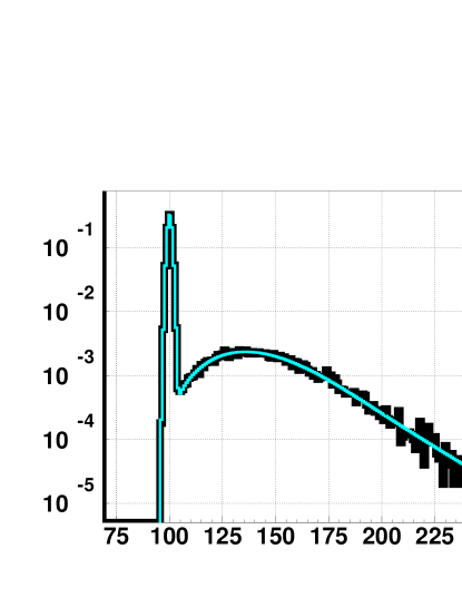
ADC counts   

Table 2: Monte Carlo input compared with mean and RMS of the results from fits to 128 simulated spectra, with $\lambda_{1}=0.15$

	MC input	Mean fit result $\pm$ RMS spread
$\lambda_{1}$	0.150	0.1501$\pm$	0.0013
$g_{1}$	5.000	5.0012$\pm$	0.058
$p_{0}$	100.00	99.999$\pm$	0.0038
$\sigma$	1.0000	1.0004$\pm$	0.0027
$c_{n}$	$3.20\cdot 10^{-4}$	$(3.23$$\pm$	$0.46)\cdot 10^{-4}$

Figure 2: MC–generated PMT ADC–spectrum, from 100k events, with $\lambda_{1}=3$. The fit is superimposed.

$10^{5}$ events / ADC–count  

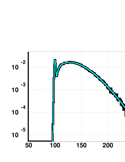
ADC counts   

Table 3: Monte Carlo input compared with mean and RMS of the results from fits to 128 simulated spectra (representing 2 64–channel MaPMT’s), with $\lambda_{1}=3$

	MC input	Mean fit result $\pm$ RMS spread
$\lambda_{1}$	3.000	3.002$\pm$	0.022
$g_{1}$	5.000	4.985$\pm$	0.107
$p_{0}$	100.000	99.999$\pm$	0.021
$\sigma$	1.000	0.999$\pm$	0.016
$c_{n}$	$6.4\cdot 10^{-4}$	$(6.45$$\pm$	$0.17)\cdot 10^{-4}$

The fit results agree very well with the input values, as shown in tables 2 and 3. To test the sensitivity of the fit result on the exact knowledge of $\alpha$, the fit to the spectrum in figure 1 is repeated assuming different values for this parameter in the fit–function: $\alpha=0.5$ and $\alpha=1.0$. The results are given in table 4.

Table 4: Monte Carlo input compared with fit–result for the MC–generated pulse height spectrum shown in figure 1, using different assumptions in the fit.

	MC input $\alpha=0.75$	Fit result $\alpha=0.75$	Fit result $\alpha=0.5$	Fit result $\alpha=1$	Fit result: 3 indep. dyn’s
$\lambda_{1}$	0.1500	0.1490	0.1491	0.1489	0.1492$\pm$	0.0013
$g_{1}$	5.00	5.039	4.852	5.291	4.74$\pm$	0.44
$g_{2},g_{3},g_{12}$	$g_{1}\cdot(\frac{2}{3})^{\alpha}=3.69$				4.51$\pm$	1.35
$g_{4},\ldots,g_{11}$	$g_{1}\cdot(\frac{1}{3})^{\alpha}=2.19$				1.97$\pm$	0.21
$p_{0}$	100.000	100.000	100.000	100.000	100.000$\pm$	0.003
$\sigma$	1.0000	1.0028	1.0029	1.0027	1.0028$\pm$	0.0025
$c_{n}$	$3.20\cdot 10^{-4}$	$2.90\cdot 10^{-4}$	$0.373\cdot 10^{-4}$	$19.7\cdot 10^{-4}$	$(4.37\pm 0.98)\cdot 10^{-4}$

Another fit was performed that does not use the formula $g\propto V^{\alpha}$. Here it is only assumed that dynodes with the same accelerating voltage have the same gain. Instead of one gain, three gains need to be fitted, one for each accelerating voltage. The fits are performed using the function minimisation and error analysis package MINUIT [Jam94]. The results from this fit, with error–estimates provided by MINUIT, are given in the last column of table 4.

Comparing the results for the different assumptions shows that they have little impact on the the fitted value for the number of photo electrons and the gain at the first dynode. Most of the error introduced by an incorrect estimate of the parameter $\alpha$ is absorbed into the ratio of ADC–counts to electrons, $c_{n}$, while the values for $\lambda_{1}$ and $g_{1}$ come out close to the input values.

4.2 Application to Testbeam Data

The fit method has been applied to spectra obtained from a prototype RICH detector, incorporating an array of nine 64–channel Hamamatsu PMTs and operated in a CERN testbeam [RIC00]. Fits were performed to estimate the signal loss at the first dynode and below the threshold cut.

Figure 3: Data from 6k events in black, with fit superimposed. The dashed line indicates the single photoelectron contribution. The signal loss refers to the fraction of photoelectrons lost below the threshold cut; both the total fraction of photoelectrons, and the fraction of single photoelectron events lost below the cut is given. These numbers do not include the loss at the first dynode due to photoelectrons producing zero secondary electrons.

events / ADC–count

   

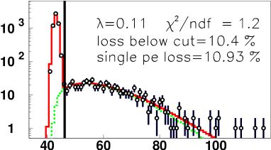
ADC counts  

Table 5: Result of fit applied to testbeam data

	Fit result
$\lambda_{1}$	0.107$\pm$	0.005
$g_{1}$	3.60$\pm$	0.20
$p_{0}$	43.06$\pm$	0.01
$\sigma$	0.724$\pm$	0.008
$c_{n}$	$(61$$\pm$	$30)\cdot 10^{-4}$

Figure 3 shows an example of such a fit to a spectrum obtained in the testbeam. The fit describes the data well, with a $\chi^{2}/\mathsf{dgf}$ of 1.2. The line in figure 3 marks the threshold cut used for photon counting in the testbeam. The fraction of single photoelectron events below that cut is $\sim 10\%$ (this does not include the irrecoverable loss of photoelectrons that do not produce any secondaries in the first dynode).

4.3 Background

Figure 4: MC–simulated PMT spectrum with background; the fit result is superimposed

events / ADC–count

   

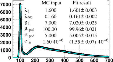
ADC counts  

Figure 5: The different contributions to the fit in figure 4

events / ADC–count

   

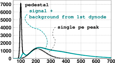
ADC counts  

Apart from the Gaussian noise taken into account here, various other sources of background, such as electrons released due to the photoelectric effect in the first dynode, thermal electrons from the photocathode or the dynodes, genuine photoelectrons missing the first dynode, etc, can contribute to a PMT pulse height spectrum. A detailed discussion of such background is beyond the scope of this paper. However, any type of background that originates from within the dynode chain can be naturally accomodated in the fit method described here, since this background undergoes the same type of amplification process as the signal. To illustrate this, a spectrum has been generated with a Monte Carlo program, assuming a signal of $1.6$ photoelectrons per event and a background of $0.16$ photoelectrons per event due to the photoelectric effect in the first dynode (see [CZ⁺01] for a fit to real data showing this kind of background, using a different method). The function to fit this spectrum is obtained by convoluting the background–free function $P(k)$ with another function $P_{\mathrm{bg}}(k)$. $P_{\mathrm{bg}}(k)$ is identical to $P(k)$ except that the amplification due to the first dynode is missing and that the number of photoelectrons per event hitting the second dynode, $\lambda_{\mathrm{bg}}$, is a new free parameter. In the example given here, $P$ and $P_{\mathrm{bg}}(k)$ are calculated to give the exact distributions for signal and background respectively after the fourth dynode; then the two distributions are convoluted and the result is scaled according to equation 34. The generated spectrum and the fit result are shown in figure 4; the fit function is shown again in figure 5 showing the non–pedestal and the single photoelectron contributions separately.

5 Summary

An analytical formula for the the probability distribution of the number of electrons at the end of a dynode chain, or any “snowball” like process described by a series of Poisson distributions, is derived. The formula describes the amplification process at all stages exactly, in particular without approximating Poisson distributions with Gaussians. It is evaluated as a function of the number of photoelectrons coming from the cathode and the gains at each dynode. The initially found formula is adapted to reduce numerical problems due to the multiplication of very large numbers with very small ones. A numerical recipe is given that implements that function.

It is shown how the function can be used as the core element of an approximated, but faster algorithm, that calculates the exact distribution for the first few dynodes and then scales the result according to the gain at the remaining dynodes, approximating the additional spread at those dynodes with a Gaussian. The number of dynodes for which the distribution is calculated exactly is not limited in principle and can be adjusted according to the precision required, and the computing time available. It is also shown how to modify the function to describe ADC–spectra obtained from read–out electronics, rather than directly the number of electrons at the end of a dynode chain.

This fast algorithm is then used to fit Monte Carlo generated ADC–spectra. In the fit function, the electron distribution after the first four out of twelve dynodes is calculated exactly. The fit results reproduce the MC–input values well. The dependence of the fit result on the assumptions made to reduce the number of fit–parameters is investigated. These results show that the fitted value for the number of photoelectrons per event is very weakly dependent on the different assumptions considered here, and the fitted gain on the first dynode also does not depend strongly on them. Real data from a multi–anode PMT used in the 1999 LHCb–RICH testbeam are fitted, and shown to be described well by the function. Finally it is illustrated how the fit function can be modified further to accommodate background from within the dynode chain, using the example of the photoelectric effect in the first dynode.

Appendix A FORTRAN Routine to Calculate $P(k_{n})$

*

      SUBROUTINE DYNODE_CHAIN(OUT, MAX, LAMBDA, DYNODES)
      IMPLICIT NONE
*     This program takes as its input the maximum number of electrons at
*     the end of the dynode chain, for which it should calculate P(k_n),
*     MAX, the average number of photo-electrons hitting the first
*     dynode, LAMBDA(1), the gains at each dynode, LAMBDA(2),
*     ... LAMBDA(DYNODES) and the dimension of the array LAMBDA:
*     DYNODES. It calls the routine MAKE_P_RATIO, which is listed at the
*     end of this file.
*
*     The output is put into the array OUT(MAX), where the probability
*     to find k_n < MAX electrons at the end of the dynode chain is
*     given by OUT(k_n).
*
*     Written by Jonas Rademacker.
*
      INTEGER MAX, DYNODES
      DOUBLE PRECISION OUT(0:MAX), LAMBDA(DYNODES)

      INTEGER ABS_MAX, MAX_DYN
      PARAMETER(ABS_MAX=50001,MAX_DYN=13)

      INTEGER IX,IY,M,I, K, J

*     To avoid having to define a limit on the number k_n that can be
*     calculated, one could create these arrays outside the program and
*     pass them on.
      DOUBLE PRECISION F(1:MAX_DYN) ! corrsponds to f^{star} in the text
      DOUBLE PRECISION U(1:MAX_DYN,0:ABS_MAX),V(1:MAX_DYN,0:ABS_MAX)
      DOUBLE PRECISION X(1:MAX_DYN)

      DOUBLE PRECISION FASTNULL
      PARAMETER (FASTNULL=1.d-300)

      DOUBLE PRECISION MEAN

      DOUBLE PRECISION P_ratio(ABS_MAX), F_FACTOR, U_FACTOR, V_FACTOR

      INTEGER MAX_OLD
      SAVE MAX_OLD
      DATA MAX_OLD/-9999/

      SAVE P_ratio

*     -- Some initialisations and tests --
      DO IX=1,MIN(ABS_MAX,MAX),+1
         OUT(IX)=0.d0
      ENDDO
      IF(ABS_MAX.LT.MAX)THEN
         RETURN
      ENDIF
      MEAN = 1.D0
      DO IX=1,DYNODES,+1
         MEAN = MEAN*LAMBDA(IX)
      ENDDO
      IF(MEAN.LE.0.d0)THEN
         OUT(0)=1.d0
         RETURN
      ENDIF

*     -- make and save the factors P_ratio(k)=(p_{k}/p_{k-1})^{k} --
      IF(MAX.GT.MAX_OLD)THEN
         MAX_OLD=MAX
         CALL MAKE_P_RATIO(P_ratio,MAX)
      ENDIF

*     -- Calculate the probability to see zero electrons (k_n=0) --
      F(DYNODES)=1.d0
      U(DYNODES,0)=F(DYNODES)
      V(DYNODES,0)=F(DYNODES)
      DO IX=DYNODES-1,1,-1
         X(IX)   = LAMBDA(IX)*DEXP(-LAMBDA(IX+1))
         F(IX)   = DEXP(X(IX)*F(IX+1))
         U(IX,0) = F(IX)
         V(IX,0) = F(IX)
      ENDDO
      OUT(0)=DEXP(-LAMBDA(1))*F(1) !   <---- save the result

*     -- Calculate the probabilities for k_n=1,...,MAX electrons --
      DO K=1,MAX,+1
*     .  calculate f_n
         IF(F(DYNODES).LT.FASTNULL)THEN
            F(DYNODES)=0.d0
         ELSE
            F(DYNODES)=F(DYNODES) * LAMBDA(DYNODES)/DBLE(K)
         ENDIF
         U(DYNODES,K)=F(DYNODES)
         V(DYNODES,K)=F(DYNODES)

*     .  re-calculate U and V from previous iteration:
         DO J=0,K-1,+1
            F_FACTOR=P_ratio(K)**(DBLE(J)/DBLE(K))
            IF(K-1-J.GT.0)THEN
               U_FACTOR=DSQRT(DBLE(K-1)/DBLE(K-1-J))*
     &              F_FACTOR
            ELSE
               U_FACTOR=F_FACTOR
            ENDIF
            V_FACTOR=DSQRT((DBLE(K-1)/DBLE(K-J)))*
     &           F_FACTOR

            DO I=DYNODES,1,-1
               U(I,J)=U(I,J)*U_FACTOR
               V(I,J)=V(I,J)*V_FACTOR
            ENDDO
         ENDDO

*     .  apply the recursive formula to get f^{k}_i
         DO I=DYNODES-1, 1, -1
            F(I)=0.d0
            DO J=0,K-1
               F(I)=F(I)+U(I,K-1-J)*X(I)*V(I+1,J+1)
            ENDDO
            U(I,K)=F(I)
            V(I,K)=F(I)
         ENDDO
*     .  calculate P(k):
         OUT(K)=DEXP(-LAMBDA(1))*F(1) !   <---- save the result
      ENDDO

      RETURN
      END

*__________________________________________________________________
      SUBROUTINE MAKE_P_RATIO(P_ratio,MAX)
      IMPLICIT NONE
      INTEGER MAX
      DOUBLE PRECISION P_ratio(MAX)

      INTEGER N
      DOUBLE PRECISION NFAC

      DOUBLE PRECISION PI, E
      PARAMETER(PI=3.1415927d0, E=2.718281828d0)

      INTEGER APPROX_FROM
      PARAMETER(APPROX_FROM=25)

      NFAC=1.D0
      P_ratio(1)=1.d0
      DO N=2,MIN(APPROX_FROM-1,MAX),+1
         NFAC=NFAC*DBLE(N-1)
         P_ratio(N)=(NFAC**(1.d0/DBLE(N-1)))/DBLE(N)
      ENDDO

      DO N=APPROX_FROM,MAX,+1
         P_ratio(N)=
     &        (2.D0*PI*DBLE(N-1))**(1.D0/(2.D0*DBLE(N-1)))*
     &        DBLE(N-1)/(E*DBLE(N))*
     &        (1.d0+1.d0/DBLE(12*(N-1))+
     &        1.d0/DBLE(288*(N-1)**2)
     &        )**(1.D0/DBLE(N-1))
      ENDDO

      RETURN
      END

*________________________________________________________________
*

References

- [CZ+01] I. Chirikov-Zorin et al. Method for precise analysis of the metal package photomultiplier single photoelectron spectra. Nucl. Instrum. Meth., A456:310, 2001.
- [Ham00] Hamamatsu Book on Photo Multipliers, September 2000.
- [Jam94] F. James. MINUIT Function Minimization and Error Analysis. Reference Manual. Version 94.1, March 1994. CERN Program Library Long Writeup D506.
- [RIC00] LHCb RICH, Technical Design Report, September 2000. CERN/LHCC/2000-0037.