Abstract

We give an account of the appearance and first developments of the statistical model of atoms proposed by Thomas and Fermi, focusing on the main results achieved by Fermi and his group in Rome. Particular attention is addressed to the unknown contribution to this subject by Majorana, anticipating some important results reached later by leading physicists.

1 Introduction

In the occasion of the centennial of the death of A. Volta, an important international conference was held in Como (Italy) on September 1927, mainly devoted to the principles and applications of the new Quantum Mechanics. Among the interesting contributions by Bohr, Heisenberg, Pauli and others, it stands out the long speech by Fermi aimed to point out the different behavior of the particles satisfying the Bose-Einstein statistics and those obeying the Pauli exclusion principle, such as electrons. Fermi started to investigate in this direction since 1923 [1], [2], when he published his “remarks on the quantization of systems with identical particles”, where anticipated the formulation of the exclusion principle for generic molecules given by Pauli one year later. Soon after the appearance of the Pauli paper, Fermi recognized to have all the tools in order to build a theory of perfect gases satisfying the Nernst principle at zero temperature, and on the 7th February, 1926 he presented the statistical distribution law for particles obeying the exclusion principle [3]. Such a law will be independently discovered later by Dirac in the August of the same year. The most distinguished physicists of that epoch reached immediately the importance of the Fermi work, and in the February of 1927 Pauli applied it to the conduction electrons in a metal, explaining their anomalous paramagnetism. Later on, at the Como conference, Sommerfeld reported on his recent works on thermal and transport properties in metals and succeeded in explaining, for the first time, the electron contribution to the specific heat of a metal. Probably encouraged by the successful application to specific heat and entropy calculations, in the fall of 1927, just after the Como conference, Fermi matured the idea of applying his statistical method to the completely degenerate state of the electrons in an atom, in order to evaluate the effective potential acting on the electrons themselves. He was aware of the fact that, since the number of the electrons involved is usually only moderately large, the results obtained will not present a very high accuracy. Nevertheless, the method resulted to be very simple, and gave an easy-to-use expression for the screening of the Coulomb potential accounted for by electrons as a whole.

Then Fermi started to apply his method to several problems of atomic physics, and some more were suggested at that time to Rasetti and other associates of his group in Rome. The basic idea of the statistical method of atoms became one of his preferred ones, and practically the main activity of the Fermi group at the Physics Institute in Rome from 1928 to 1932 was devoted to this subject.

2 The Thomas-Fermi model

2.1 The case of neutral atoms

The main idea of the statistical model of atoms is that of considering the electrons around the atomic nucleus as a gas of particles, obeying the Pauli exclusion principle, at the absolute zero of temperature. The limiting case of the Fermi statistics for strong degeneracy applies to such a gas. Then, the maximum electron kinetic energy (in a neutral atom),

$$\frac{p_{0}^{2}}{2m}=e\,V,$$ (1)

can be identified with that of a uniform gas of electrons whose number density is given by:

$$n=\frac{8\pi p_{0}^{3}}{3h^{3}},$$ (2)

Note that the total energy has to be constant at any spatial point since, otherwise, a flux of electrons from one point to another would be established. The potential energy $-eV$ depends, thus, on the position through the electron charge density $\rho=-en$ at that point:

$$\rho=-\frac{1}{3\pi^{2}}\left(\frac{2\,m}{\hbar^{2}}\right)^{3/2}(e\,V)^{3/2}.$$ (3)

This was realized by Thomas in 1926 [4] and, independently, by Fermi in the December of 1927 [5]. Fermi and many other relevant physicists were unaware that essentially identical conclusions had previously been reached by Thomas, since the English researcher published his results on a journal which was probably not widespread through the physics community. According to Rasetti [6], “Fermi became acquainted with Thomas’ paper only late in 1928, when it was pointed out to him by one (now unidentified) of the foreign theoreticians visiting Rome”. It is also intriguing to note that for some time the statistical model was denoted as the Fermi-Thomas model rather then as the Thomas-Fermi one (compare, for example the papers in Refs [7],[8] appeared in 1930 with that of Sommerfeld in [9] of 1932). We further observe that Thomas made use of only the exclusion principle (in writing Eq. (2), while Fermi considered also the dependence of the effective potential (entering in Eq. (3)) on the temperature of the gas. Such a difference, however, is not very significative since the number density of electrons in the occupied states of an atom reaches high values due to the small space region where they are placed. Then, the electrons form a completely degenerate gas, and the correction to the effective potential reduces to a small term proportional to the temperature $T$, which does not alter the main results of the model in the limit $T\rightarrow 0$.

The effective electrostatic potential is related to the electron charge density by means of the Poisson equation,

$$\nabla^{2}V=-4\pi\rho,$$ (4)

and substituting in this the expression in Eq. (3), Thomas and Fermi found a second-order inhomogeneous differential equation for $V$ with a term proportional to $V^{3/2}$:

$$\nabla^{2}V=\frac{4e}{3\pi}\left(\frac{2\,m}{\hbar^{2}}\right)^{3/2}(e\,V)^{3/2}.$$ (5)

This equation allows the evaluation of the potential inside an atom with atomic number $Z$, using boundary conditions such that for the radius $r\rightarrow 0$ the potential becomes the Coulomb field of the nucleus,

$$V(r)\rightarrow\frac{Ze}{r},$$ (6)

while for $r\rightarrow\infty$:

$$V(r)\rightarrow 0.$$ (7)

The additional condition for the total charge,

$$\int n\,d^{3}{\mathbf{r}}=Z,$$ (8)

is automatically satisfied, provided that Eqs. (6) and (7) hold.

In order to simplify the differential equation in Eq. (5), Fermi introduced a suitable change of variables:

$$\begin{array}[]{rcl}r&=&\mu x\\ &&\\ V(r)&=&\displaystyle\frac{Ze}{r}\varphi(r)\end{array}$$ (9)

with

$$\mu=\frac{1}{2}\left(\frac{3\pi}{4}\right)^{2/3}\frac{\hbar^{2}}{me^{2}}Z^{-1/3}.$$ (10)

In terms of the new variables, Eq. (5) becomes (for $\varphi>0$):

$$\varphi^{\prime\prime}=\frac{\varphi^{3/2}}{\sqrt{x}}$$ (11)

(a prime denotes differentiation with respect to $x$) with the boundary conditions:

$$\begin{array}[]{rcl}\varphi(0)&=&1,\\ &&\\ \varphi(\infty)&=&0.\end{array}$$ (12)

The Fermi equation (11) is a universal equation which does not depend neither on $Z$ nor on physical constants ($\hbar,m,e$). Its solution gives, from Eq. (9), as noted by Fermi himself, a screened Coulomb potential which at any point is equal to that produced by an effective charge

$$Ze\,\varphi\left(\frac{r}{\mu}\right).$$ (13)

As was immediately realized, in force of the independence of Eq. (11) on $Z$, the method gives an effective potential which can be easily adapted to describe any atom with a suitable scaling factor, according to Eq. (13).

2.2 The case of positive ions

In order to evaluate ionization energies and similar quantities which are relevant for Atomic Physics observations, Fermi and Rasetti [6], [10], [11] proceeded to apply and enlarge the above method to describe positive ions. They considered the ion of nuclear charge $Ze$ as a neutral atom of nuclear charge $(Z-1)e$, to be treated with the statistical method, plus an extra proton in the nucleus.

Since the electrostatic potential for the atom of atomic number $Z-1$ is, from (13),

$$\frac{(Z-1)e}{r}\,\varphi\left(\frac{r}{\mu}\right).$$ (14)

(with $Z\rightarrow Z-1$ for the parameter $\mu$ in Eq. (10)), the potential energy of one extra electron will be, at a first approximation, given by:

$$-eV=-\frac{e^{2}}{r}\left[1+(Z-1)\,\varphi\left(\frac{r}{\mu}\right)\right].$$ (15)

With this formula, Fermi and his associates in Rome extended their calculations to many physical problems, obtaining quantities which well fitted the observations and the knowledge of the time.

The method was further generalized for arbitrary positively charged ions by Baker in June 1930 [7] and corrected (for an interpretational misunderstanding) by Guth and Peierls six months later [8].

3 Solution of an equation

3.1 Numerical works

The problem of the theoretical calculation of observable atomic properties is solved, in the statistical model approximation, in terms of the function $\varphi(x)$ introduced in Eq. (9) and satisfying the Fermi differential equation (11). However, it was believed that the solution of such equation satisfying the appropriate boundary conditions in (12) couldn’t be expressed in closed form, so that some effort was made by Thomas [4], Fermi [5], [11] and others [7] in order to achieve numerical integration of the differential equation.

Thomas used a numerical method described by Whittaker and Robinson [12] in order to solve the second-order differential equation for the electrostatic potential $V$. He thus obtained a numerical table for some mathematical quantities from which one can deduce the values of $V$ as function of the distance $r$ from the nucleus. However, as already observed by Baker [7], Thomas’ numerical calculations of $V$ near $r=0$ are “slightly in error”, and this influenced also some calculations by Milne [13] who directly applied the Thomas theory as early as in 1927.

A similar effort was also pursued by Fermi who built a numerical table for the values of the function $\varphi(x)$ obeying Eq. (11). The numerical work was performed in approximately one week and, according to many testimonies [6], [14] (see the anecdote related to Majorana), the table was ready as early as at the end of 1927, although it was published only in the German paper of 1928 [11]. The numerical values obtained by Fermi were largely used not only by the members of the Rome group, but even by many other physicists who dealt with atomic problems (see, for example, Refs. [7],[15]).

3.2 Approximate solutions in two limiting cases

By using standard but involved mathematical tools, in his paper [4] Thomas got an exact, “singular” solution of his differential equation satisfying only the condition (7). This was later (in 1930) considered by Sommerfeld [15] as an approximation of the function $\varphi(x)$ for large $x$ (and is indeed known as the “Sommerfeld solution” of the Fermi equation),

$$\varphi(x)=\frac{144}{x^{3}},$$ (16)

and Sommerfeld himself obtained corrections to the above quantity in order to approximate in a better way the function $\varphi(x)$ for not extremely large values of $x$. The goodness of the approximated expression was checked by Sommerfeld comparing his results with the numerical values obtained by Fermi [15].

It is intriguing to observe that the solution in Eq. (16) was already known to Majorana [19] at the end of 1927 (independently from Thomas), who recognized its crucial role in determining the desired solution of Eq. (11) with boundary conditions Eq. (12) (see below).

An approximate solution for $\varphi(x)$ near $x=0$ was, instead, first considered by Fermi [5], who obtained a series expansion for it. The reasoning is, probably, as follows. For $x$ near $0$ we have $\varphi(x)\sim 1$, so that substitution into Eq. (11) results in

$$\varphi^{\prime\prime}(x)=x^{-1/2}.$$ (17)

By integrating this approximate equation we easily have

$$\varphi(x)\sim k_{1}+k_{2}x+\frac{4}{3}x^{3/2},$$ (18)

for $x$ near the origin. The constant $k_{1}$ is obtained directly from the first condition in (12), while $k_{2}$ was determined by Fermi to assume the numerical value $-1,58$ for the neutral atom. Thus, the Fermi approximation for $x\rightarrow 0$ results to be:

$$\varphi(x)=1-1.58x+\frac{4}{3}x^{3/2}+...\,.$$ (19)

According to Rasetti [6], Segrè [16] and Amaldi [14], the paper in Ref. [5] was shown to Majorana probably even before its publication. Majorana then proceeded to improve the degree of approximation of the Fermi formula (19), and considered several other terms in the series expansion up to the sixth power of $x$ (including both integer and half-integer powers). The method followed by him is a generalization of the Frobenius method for differential equations [18]; its sketch is as follows.

Let us consider a solution of Eq. (11), which can be rewritten as

$$x(\varphi^{\prime\prime})^{2}-\varphi^{3}=0,$$ (20)

in the form

$$\varphi(x)=\sum_{n=0}^{\infty}(a_{2n}\,x^{n}+a_{2n-1}\,x^{n+\frac{1}{2}}).$$ (21)

The terms in Eq. (21) with integer powers of $x$ account for the usual Taylor series expansion, while those with half-integer powers attain to the Frobenius one. The need for both terms is dictated by the Fermi approximation underlying Eqs. (17)-(19). The yet unknown coefficients $a_{2n}$ and $a_{2n-1}$ are then determined by substituting Eq. (21) into Eq. (20) and requiring that the coefficients of given powers of $x$, appearing in the L.H.S. of Eq. (20), vanish. In such a way, one is able to obtain two iterative formulae for $a_{2n}$ and $a_{2n-1}$ coefficients. However, differently from what is usually found in the notebooks by Majorana (see [17]), he did not succeed to obtain general expressions for the coefficients, but he stopped the series to the term $x^{6}$ (thus considering a polynomial) and evaluated only some coefficients. The corresponding expression looks like as follow:

$$\varphi(x) = 1-px+\frac{4}{3}x^{3/2}-\frac{2p}{5}x^{5/2}+\frac{1}{3}x^{3}+\frac{3p^{2}}{70}x^{7/2}-\frac{2p}{15}x^{4}+\frac{56+3p^{3}}{756}x^{9/2}+\frac{p^{2}}{175}x^{5}$$ (22)

$$+ \frac{-992p+45p^{4}}{47520}x^{11/2}+\frac{4(35-9p^{3})}{14175}x^{6},$$

with $p=1.58$, according to the Fermi value. Probably, Majorana abandoned the complete series expansion in (21) because he realized that such a series does not converge to the desired solution. Note, in fact, that the differential equation (11) or (20) is a non-linear equation, so that the series solution method cannot, in general, be applied at all. It is however remarkable that, stopping the series in (21) to any power $n\leq 5$, the obtained polynomial diverges towards to $+\infty$ for diverging $x$, while from $n=6$ (as considered by Majorana) onward the corresponding polynomial diverges towards $-\infty$, as can be seen in Fig.1. Both behaviors, of course, do not match the correct condition $\varphi(x\rightarrow\infty)\rightarrow 0$, but we point out that the first one, $\varphi(x\rightarrow\infty)\rightarrow+\infty$, is physically not acceptable (see, for example, the discussion in Ref. [8]). Eventually, we point out that the Fermi approximation of the function $\varphi(x)$ near $x=0$ with a polynomial was later reconsidered by Baker [7], who obtained terms up to the power $x^{9/2}$. However, the coefficient of the last term presented by author is wrong (compare with the correct Majorana result in Eq. (22)). We have dwell on this point in order to remark the complexity of calculations, leading to the expressions for the coefficients in the polynomial expansion, due to the non-linearity of the equation considered. For example, in order to evaluate the coefficients $a_{i}$ in Eq. (21) up to the term $x^{9/2}$, we have to solve a set of $10$ coupled algebraic equations. Note also that, due to the structure of the differential equation in (20), for obtaining the correct expressions for the coefficients, we have to start with a polynomial in (21) with terms up to $x^{15/2}$, rather than $x^{9/2}$.

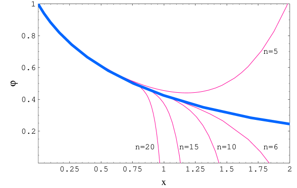
Figure 1: The Thomas-Fermi function $\varphi(x)$ (thick curve) and its Frobenius polynomial approximations for small $x$. The labels $n=5,6,10,15,20$ refer to the maximum power considered in the expansion in Eq. (21).

3.3 Exact and semi-analytical results

The work described above on the polynomial approximation, performed by Majorana, was only the first step towards an exact or semi-analytical solution to the Fermi equation. We will indulge here on an anecdote reported by Rasetti [6], Segrè [16] and Amaldi [14]. According to the last author, “Fermi gave a broad outline of the model and showed some reprints of his recent works on the subject to Majorana, in particular the table showing the numerical values of the so-called Fermi universal potential. Majorana listened with interest and, after having asked for some explanations, left without giving any indication of his thoughts or intentions. The next day, towards the end of the morning, he again came into Fermi’s office and asked him without more ado to draw him the table which he had seen for few moments the day before. Holding this table in his hand, he took from his pocket a piece of paper on which he had worked out a similar table at home in the last twenty-four hours, transforming, as far as Segrè remembers, the second-order Thomas-Fermi non-linear differential equation into a Riccati equation, which he had then integrated numerically.”

The whole work performed by Majorana on the solution of the Fermi equation, is contained in some spare sheets conserved at the Domus Galilaeana in Pisa, and diligently reported by the author himself in his notebooks [17]. The reduction of the Fermi equation to an Abel equation (rather than a Riccati one, as confused by Segrè) proceeds as follows. Let’s adopt a change of variables, from $(x,\varphi)$ to $(t,u)$, where the formula relating the two sets of variables has to be determined in order to satisfy, if possible, both the boundary conditions (12). The function $\varphi$ in Eq. (16) has the correct behavior for large $x$, but the wrong one near $x=0$, so that we could modify the functional form of $\varphi$ to take into account the first condition in (12). An obvious modification is $\varphi=(144/x^{3})f(x)$, with $f(x)$ a suitable function which vanishes for $x\rightarrow 0$ in order to account for $\varphi(x=0)=1$. The simplest choice for $f(x)$ is a polynomial in the novel variable $t$, as it was also considered later, in a similar way, by Sommerfeld [15]. The Majorana choice is as follows:

$$\varphi(x)=\frac{144}{x^{3}}(1-t)^{2},$$ (23)

with $t\rightarrow 1$ as $x\rightarrow 0$ . From Eq. (23) we can then obtain the first relation linking $t$ to $x,\varphi$. The second one, involving the dependent variable $u$, is that typical of homogeneous differential equations (like the Fermi equation) for reducing the order of the equation, i.e. exponentiation with an integral of $u(t)$. The transformation relations are thus:

$$\begin{array}[]{rcl}t&=&\displaystyle 1-\frac{1}{12}\sqrt{x^{3}\varphi},\\ &&\\ \varphi&=&e^{\int_{1}^{t}u(t)dt}\,.\end{array}$$ (24)

Substitution into Eq. (11) leads to an Abel equation for $u(t)$,

$$\frac{du}{dt}=\alpha(t)+\beta(t)\,u+\gamma(t)\,u^{2}+\delta(t)\,u^{3},$$ (25)

with

$$\begin{array}[]{rcl}\alpha(t)&=&\displaystyle\frac{16}{3(1-t)},\\ &&\\ \beta(t)&=&\displaystyle 8+\frac{1}{3(1-t)},\\ &&\\ \gamma(t)&=&\displaystyle\frac{7}{3}-4t,\\ &&\\ \delta(t)&=&\displaystyle-\frac{2}{3}t(1-t).\end{array}$$ (26)

Note that both the boundary conditions in (12) are automatically verified by the relations (24). We have reported the derivation of the Abel equation (25) mainly for historical reasons (see also the next section); the precise numerical values for the Fermi function $\varphi(x)$ were obtained by Majorana by solving a different first-order differential equation [19]. It is also remarkable that none of the Majorana’s colleagues and friends was aware of this, which however is well documented in the notebooks [17] and in some other unpublished papers. Instead of Eq. (23), Majorana chooses $\varphi(x)$ of the form

$$\varphi(x)=\frac{144}{x^{3}}\,t^{6}.$$ (27)

Now the point with $x=0$ corresponds to $t=0$. In order to obtain again a first order differential equation for $u(t)$, the transformation equation for the variable $u$ involves $\varphi$ and its first derivative. Majorana then introduced the following formulas:

$$\begin{array}[]{rcl}t&=&144^{-1/6}\,x^{1/2}\,\varphi^{1/6},\\ &&\\ u&=&\displaystyle-\left(\frac{16}{3}\right)^{1/3}\varphi^{-4/3}\varphi^{\prime}\,\,.\end{array}$$

By taking the $t$-derivative of the last equation in (3.3) and inserting Eq. (11) in it, one gets:

$$\frac{du}{dt}=-\left(\frac{16}{3}\right)^{1/3}\dot{x}\varphi^{-4/3}\left[-\frac{4}{3}\frac{\varphi^{\prime 2}}{\varphi}+\frac{\varphi^{3/2}}{x^{1/2}}\right].$$ (28)

By using Eqs. (3.3) to eliminate $x^{1/2}$ and $\varphi^{\prime 2}$, the following equation results:

$$\frac{du}{dt}=\left(\frac{4}{9}\right)^{1/3}\frac{tu^{2}-1}{t}\dot{x}\varphi^{1/3}.$$ (29)

Now the quantity $\dot{x}\varphi^{1/3}$ can be expressed in terms of $t$ and $u$ by making use again of the first equation in (3.3) (and its $t$-derivative). After some algebra, the final result for the differential equation for $u(t)$ is:

$$\frac{du}{dt}=8\,\frac{tu^{2}-1}{1-t^{2}u}.$$ (30)

The obtained equation is again non-linear but, differently from the original Fermi equation (11), it is first-order in the novel variable $t$ and the degree of non-linearity is lower than that of Eq. (11). The boundary conditions for $u(t)$ are easily taken into account from the second equation in (3.3) and by requiring that for $x\rightarrow\infty$ the Sommerfeld solution (Eq. (27) with $t=1$) be recovered:

$$\begin{array}[]{rcl}u(0)&=&\displaystyle-\left(\frac{16}{3}\right)^{1/3}\varphi^{\prime}_{0},\\ &&\\ u(1)&=&1.\end{array}$$ (31)

Here we have denoted with $\varphi^{\prime}_{0}=\varphi^{\prime}(x=0)$ the initial slope of the Thomas-Fermi function $\varphi(x)$ which, for a neutral atom, is approximately equal to $-1.588$.

The solution of Eq. (30) was achieved by Majorana in terms of a series expansion in powers of the variable $\tau=1-t$:

$$u=a_{0}+a_{1}\tau+a_{2}\tau^{2}+a_{3}\tau^{3}+...\,\,.$$ (32)

Substitution of Eq. (32) (with the conditions in Eq. (31)) into Eq. (30) results into an iterative formula for the coefficients $a_{n}$ (for details see Ref. [19]). It is remarkable that the series expansion in Eq. (32) is uniformly convergent in the interval $[0,1]$ for $\tau$, since the series $\sum_{n=0}^{\infty}a_{n}$ of the coefficients converges to a finite value determined by the initial slope $\varphi^{\prime}_{0}$. In fact, by setting $\tau=1$ ($t=0$) in Eq. (32) we have from Eq. (31):

$$\sum_{n=0}^{\infty}a_{n}=-\left(\frac{16}{3}\right)\varphi^{\prime}_{0}$$ (33)

Majorana was aware [17] of the fact that the series in Eq. (32) exhibits geometrical convergence with $a_{n}/a_{n-1}\sim 4/5$ for $n\rightarrow\infty$.

Given the function $u(t)$, we now have to look for the Thomas-Fermi function $\varphi(x)$. This was obtained in a parametric form $x=x(t)$, $\varphi=\varphi(t)$ in terms of the parameter $t$ already introduced in Eq. (3.3), and by writing $\varphi(t)$ as

$$\varphi(t)=e^{\int_{0}^{t}w(t)dt}$$ (34)

(with this choice, $\varphi(t=0)=1$ and the first condition in (12) is automatically satisfied). Here $w(t)$ is an auxiliary function which is determined in terms of $u(t)$ by substituting Eq. (34) into Eq. (3.3). As a result, the parametric solution of Eq. (11), with boundary conditions (12), takes the form:

$$\begin{array}[]{rcl}x(t)&=&144^{1/3}\,t^{2}\,e^{2{\cal I}(t)}\\ &&\\ \varphi(t)&=&e^{-6\,{\cal I}(t)}\end{array}$$ (35)

with

$${\cal I}(t)=\int_{0}^{t}\frac{ut}{1-t^{2}u}\,dt$$ (36)

Remarkably, the Majorana solution of the Thomas-Fermi equation is obtained with only one quadrature and gives easily obtainable numerical values for the electrostatic potential inside atoms. By taking into account only $10$ terms in the series expansion for $u(t)$, such numerical values approximate the values of the exact solution of the Thomas-Fermi equation with a relative error of the order of $0.1\%$ [19].

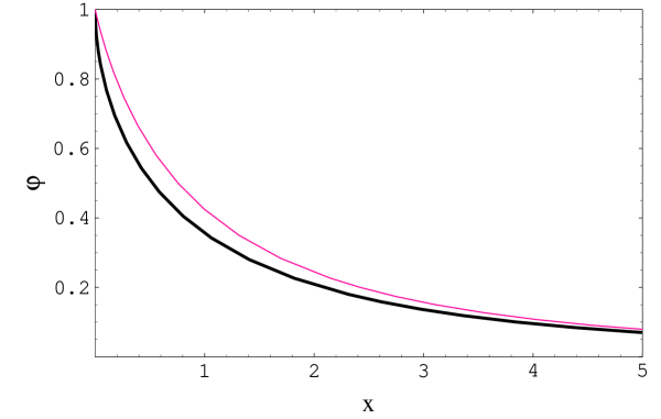
Figure 2: The Thomas-Fermi function $\varphi(x)$ and the Majorana approximation of it. The thin (upper) line refers to the exact (numerical) solution of Eq. (11) while the thick (lower) one corresponds to the parametric solution obtained from Eqs. (35)-(36).

3.4 Numerical tables

It is instructive to give a look at the numerical results for the Thomas-Fermi function $\varphi(x)$ obtained by several authors with different methods. As already pointed out, Thomas firstly reported numerical values for the potential inside atoms. Since his approach involved a differential equation equivalent to the Fermi equation but with a different mathematical structure (see [4]), which does not make direct use of the universal function $\varphi(x)$, the comparison between the Thomas numerical results and those obtained by Fermi and others will not be considered here.

It is a matter of fact that many atomic physicists in the ${}^{\prime}30$s used the Fermi table in their computations. As early as at the end of $1927$, according to Segrè [16] and Rasetti [6], Fermi obtained the values of the function $\varphi(x)$ by means of successive approximation in Eq. (11), during approximatively one week of numerical work, by using a small hand calculator (a Brunsviga one). The table, however, was published later in a German paper [11]; we reproduce in Table 1 some of these results. As pointed out above, Majorana checked the Fermi results by using probably the parametric solution in Eqs. (35). Note that only the integration in Eq. (36) requires numerical evaluation. The results obtained by Majorana, during approximatively one night of numerical work, are reported in his “Volumetti” [17] and are reproduced here in Table $1$.

A rapid look at this table shows a satisfactory agreement between the Fermi numerical approach and the Majorana method. It is even remarkable that, for the first points, Majorana obtained also the values for the derivative of the function $\varphi(x)$ (see [17]). Subsequent more accurate numerical evaluations of the solution of the Thomas-Fermi equation were performed by Miranda in $1934$ [20], who also gave a solid mathematical framework to the numerical integration of the Fermi equation (see the next section). By using refined approximation procedures to a finite variation equation corresponding to the Fermi differential equation, he obtained numerical values for $\varphi(x)$ (and $\varphi^{\prime}(x)$) which are accurate up to the fifth significant digit for small $x$ (Fermi and Majorana results are accurate “only” up to the third significant digit in the same $x$ interval). Some results (corresponding to an initial slope of $-1.5880464$) are reproduced here in Table 1 for comparison.

Table 1: Numerical values of the function $\varphi(x)$ taken from the Fermi, Majorana and Miranda papers.

$x$	$\varphi_{\rm Fer}$
0	1
0.1	0.882
0.2	0.793
0.3	0.721
0.4	0.660
0.5	0.607
0.6	0.562
0.7	0.521
0.8	0.485
0.9	0.453
1	0.425
1.2	0.375
1.4	0.333
2	0.244
3	0.157

$\varphi_{\rm Maj}$ 1 0.882 0.793 0.721 0.660 0.607 0.561 0.521 0.486 0.453 0.424 0.374 0.333 0.243 0.157 $\varphi_{\rm Mir}$ 1 0.88170 0.79307 0.72065 0.65955 0.607 0.56118 0.52081 0.48495 0.45288 0.42403 0.37427 0.33294 0.24306 0.15675       $x$ $\varphi_{\rm Fer}$ 4 0.108 5 0.079 6 0.059 7 0.046 8 0.037 9 0.029 10 0.024 20 0.0056 30 0.0022 40 0.0011 50 0.00061 60 0.00039 80 0.00018 100 0.0001 $\varphi_{\rm Maj}$ 0.108 0.079 0.059 0.046 0.036 0.029 0.024 0.0056 0.0022 0.0011 0.0006 0.0004 0.0002 0.0001 $\varphi_{\rm Mir}$ 0.1086 0.0798 0.0599 0.0469 0.038 0.030 0.025 0.0063 0.0024 0.0012 0.00068 0.00042 0.00019 0.0001

A remarkable agreement between the results given by the three authors, which used completely different techniques, can be clearly deduced.

3.5 Mathematical properties

The non-linear second-order differential equation (11) has received much attention by physicist from its discovery until now, mainly due to the important physical model underlying it, which is not limited to atoms [21]. On the mathematical side, some formal properties of the solutions of the Thomas-Fermi equation have been studied as well. We will give here a brief account of the results achieved in the literature, excluding from our discussion those corresponding to asymptotic expressions and theorems on numerical approximations, which have been already considered above.

From the mathematical point of view, the starting most important result for a non-linear differential equation is the theorem establishing the existence and uniqueness of its solutions. For the case considered here, we point out that the physically interesting solutions of Eq. (11) are those satisfying the boundary conditions (12) (or similar ones for electrically charged ions).

The studies performed by Majorana and described above, especially those aimed to transform the Thomas-Fermi equation into an Abel equation, seem to leave little space to speculations in this direction. In fact, the theorem of existence and uniqueness for $\varphi(x)$ directly follows from that holding for the Abel equation (25), allowing the integrability of its solution $u(t)$ which is required in Eqs. (24).

However, the Majorana work on the Thomas-Fermi equation was practically unknown to everybody (until recent times [17], [19]), and some other subsequent papers are usually quoted in the literature. The theorem of existence and uniqueness for Eq. (11) with conditions (12) was clearly stated in $1929$ by two Italian mathematicians, Mambriani [22] and Scorza-Dragoni [23]. Looking at the analytical properties of the function appearing in the R.H.S. of Eq. (11) and using standard methods holding for ordinary differential equations, they showed that an infinite number of integral curves of Eq. (11) pass through a given point $(x_{0},\varphi_{0})$ of the first quadrant of the $x-\varphi$ plane, only one of which $\varphi^{*}(x)$ being always decreasing and approaching the $x$-axis. This solution corresponds to a “critical” value of the initial slope $\varphi^{\prime}_{0}$, given by $-1.588$. The other solutions with an initial slope greater than the critical value lie above $\varphi^{*}(x)$ and diverge for diverging $x$, while those with an initial slope lower than the critical value lie below $\varphi^{*}(x)$ and monotonically decrease for increasing $x$ as far as they reach the $x-$axis.

Mambriani and Scorza-Dragoni also gave a generalization of the theorem above applicable to a given class of differential equations [22], [23]. It is also interesting to point out how several mathematicians participated in the debate originated by the discussion of the Thomas-Fermi differential equation, including Caccioppoli as quoted in [23].

Some other mathematical questions underlying the statistical model introduced by Thomas and Fermi and the solutions of the corresponding equation were then tackled only later in the $1940$’s [24]. In particular the attention drifted towards variational methods applied to a “Thomas-Fermi energy functional”, involving the screened potential $\varphi(x)$, in order to obtain the ground state energy for the relevant atoms (and molecules). A renewed interest started in $1969$ with the paper by Hille [25], who studied analytically a number of mathematical aspects of the Thomas-Fermi equation for the atomic case. Generalization to the molecular case was subsequently analyzed by Lieb and Simon in $1977$ [26], proving the existence and uniqueness of the corresponding Thomas-Fermi function.

We address the interested reader to the quoted literature for the details on this subject, which is beyond the aims of the present paper.

4 First applications of the statistical method

The first practical applications of the Thomas-Fermi model of atoms were developed by Fermi himself and his collaborators in Rome (mainly Rasetti [27], Gentile and Majorana [28]). According to Rasetti [6], “this work had been the main activity of the Rome Institute in 1928”. As outlined in Sect. 2, the electrostatic potential inside an atom of atomic number $Z$, at a distance $r$ from the nucleus, can be cast in the form:

$$V(r)=\frac{Ze}{r}\varphi\left(\frac{r}{\mu}\right),$$ (37)

where $\varphi$ is the Fermi function discussed above and $\mu$ is given in Eq. (10). Based on this, Fermi [29] calculated the number of electrons in an atom with given values of the orbital angular momentum as function of the atomic number $Z$ , thus succeeding to give an account of the appearance of the elements in the periodic table. Of course it was readily realized that, since the potential $V(r)$ was determined by means of statistical arguments, only average properties of the periodic system can be explained in terms of the Thomas-Fermi model. Peculiarities of the electronic structure, underlying particular properties of the elements, cannot be accounted for by a statistical method. Nevertheless, as noted by Fermi himself, the agreement with the experimental observations is satisfactory.

The next step was to evaluate the energy levels of the quantum states of all (heavy) elements. This was done by Fermi in [10] for the S-levels; in particular he calculated the Rydberg correction for the S-levels of any element from the approximate solution of the Schrödinger equation for an s-electron with zero energy. The energy levels corresponding to the angular momentum $l=3,m=2$ (M-levels) for the X-ray spectrum were, instead, considered by Rasetti [27]. Again the experimental points fluctuate closely about the predicted values. A slightly different application of the Thomas-Fermi potential was carried out by Gentile and Majorana [28], who calculated the doublet separation due to spin for optical and X-ray levels of some elements, applying the Dirac theory. Moreover they also evaluated the ratio of the intensities of the absorption s-p lines in the alkali spectra. Some further applications were performed by the Fermi group during $1928$, mainly devoted to explain the properties of the rare earths and the electron affinity of the halogens, which were discussed in a restricted conference in Leiprig under the chairmanship of P. Debye [11].

Several generalization of the Thomas-Fermi method for atoms were proposed as early as in $1928$ by Majorana, but they were considered by the physics community, ignoring the Majorana unpublished works, only many years later (see, for example, the review in [30]).

Indeed, in Sect. 16 of Volumetto II [17], Majorana studied the problem of an atom in a weak external electric field $E$, i.e. atomic polarizability, and obtained an expression for the electric dipole moment for a (neutral or arbitrarily ionized) atom.

Furthermore, he also started to consider the application of the statistical method to molecules, rather than single atoms, studying the case of a diatomic molecule with identical nuclei (see Sect. 12 of Volumetto II [17]). The effective potential in the molecule was cast in the form:

$$V=V_{1}+V_{2}-\alpha\,\frac{2V_{1}V_{2}}{V_{1}+V_{2}},$$ (38)

$V_{1}$ and $V_{2}$ being the potentials generated by each of the two atoms. The function $\alpha$ must obey the differential equation for $V$,

$$\nabla^{2}V=-kV^{3/2}$$ (39)

($k$ is a suitable constant), with appropriate boundary conditions, discussed in [17]. Majorana also gave a general method to determine $V$ when the equipotential surfaces are approximately known (see Sect. 12 of Volumetto III [17]). In fact, writing the approximate expression for the equipotential surfaces, as functions of a parameter $p$, as

$$f(x,y,z)=p,$$ (40)

he deduced a thorough equation from which it is possible to determine $V(\rho)$, when the boundary conditions are assigned. The particular case of a diatomic molecule with identical nuclei was, again, considered by Majorana using elliptic coordinates in order to illustrate his original method [17].

5 Conclusions

In this paper we have depicted the genesis and the first developments of the statistical model of atoms introduced by Thomas and Fermi in 1926-27. Far from being complete, our account has focused on the results achieved by Fermi and his group in Rome, as given evidence by many articles published in widespread journals. We have also pointed out the practically unknown contribution to the model given by Majorana, who was introduced to the subject by Fermi himself. One of the major results reached by Majorana as early as in the beginning of 1928 is its solution (or, rather, methods of solutions) of the Thomas-Fermi equation. This plays an important role in the rapid and accurate determination of the effective electrostatic potential in atoms, required in physical applications, as well as in studying the mathematical properties of the differential equation itself, anticipating later (Mambriani, Scorza-Dragoni, Miranda 1929-1934) and much later (Hille 1969) achievements. Majorana works on these topics (as well as in many other ones) is contained in his notebooks [17] and was not published by the author: it is remained unknown until recent times [17]. A brief account of the statistical model of atoms, which is widely known, has been reported in Sect. 2, and follows quite closely the Fermi approach. Wide room has been made to the solution of the Thomas-Fermi equation in Sect. 3; the interested reader, looking for more technical details, can benefit from a reading of papers [19], [31]. Early applications of the Thomas-Fermi model, performed by the Fermi group (as well as some other people), essentially dealt with atomic spectroscopy, and have been discussed above in Sect. 4. Moreover we have also highlighted some completely novel (for that time) applications of the statistical model by Majorana, who employed it for studying atoms in external fields (atomic polarizability) and molecules.

From what discussed here, it is then evident the considerable contribution given by Majorana even in the achievement of the Thomas-Fermi model, anticipating, in many respects, some important results reached later by leading specialists.

Acknowledgments

The authors are indebted with Prof. E. Recami; Dr. E. Majorana jr. and Prof. A. Drago for fruitful discussions.

References

- [1] E. Fermi, “Sopra la teoria di Stern della costante assoluta dell’entropia di un gas perfetto monoatomico,” Rend. Lincei, 32, 395 (1923).
- [2] E. Fermi, “Considerazioni sulla quantizzazione dei sistemi che contengono degli elementi identici,” Nuovo Cim. 1, 45 (1924).
- [3] E. Fermi, “Sulla quantizzazione del gas perfetto monoatomico,” Rend. Lincei 3, 145 (1926). E. Fermi, “Zur Quantelung des Idealen Einatomigen Gases,” Z. Phys. 36, 902 (1926).
- [4] L.H. Thomas, “The calculation of atomic fields,” Proc. Cambr. Phil. Soc., 23, 542 (1926).
- [5] E. Fermi, “Un metodo statistico per la determinazione di alcune proprietá dell’atomo,” Rend. Lincei 6, 602 (1927).
- [6] F. Rasetti in E. Fermi Collected Papers (Note e Memorie) (University of Chicago Press, Chicago, 1962) page 277.
- [7] E.B. Baker, “The application of the Fermi-Thomas statistical model to the calculation of the potential distribution in positive ions” Phys. Rev. 36, 630 (1930).
- [8] E. Guth and R. Peierls, “Application of the Fermi-Thomas Model to Positive Ions,” Phys. Rev. 37, 217 (1931).
- [9] A. Sommerfeld, “Asymptotische Integration der Differentialgleichung des Thomas-Fermischen Atoms,” Z. Phys. 78, 283 (1932).
- [10] E. Fermi, “Sulla deduzione statistica di alcune proprietá dell’atomo. Calcolo della correzione di Rydberg per i termini S,” Rend. Lincei 7, 726 (1928).
- [11] E. Fermi, “Über die anwendung der statistischen methode auf die probleme des atombaues,” Falkenhagen, Quantentheorie und Chemie, Leipziger Vortraege 95 (1928).
- [12] E. Whittaker and G. Robinson, The Calculus of Observations (Blackie, London, 1944) page 365.
- [13] E.A. Milne, “The total energy of binding of a heavy atom,” Proc. Cambr. Phil. Soc. 23, 794 (1927).
- [14] E. Amaldi, “Ettore Majorana: Man and Scientist,” in A. Zichichi (ed.), Strong and Weak Interactions. Present problems (Acedemic Press, New York, 1966).
- [15] A. Sommerfeld, “Integrazione asintotica dell’equazione differenziale di Thomas-Fermi,” Rend. Lincei 15, 788 (1932).
- [16] E. Segré, Autobiografia di un fisico (Il Mulino, Bologna, 1995).
- [17] S. Esposito, E. Majorana jr, A. van der Merwe and E. Recami (eds.), Ettore Majorana: Notes on Theoretical Physics (Kluwer, New York, 2003).
- [18] S.L. Ross, Differential Equations (University of New Hampshire Blaisdell, Durham, 1964). G. Arfken. Mathematical Methods for Physicists (Academic Press, New York, 1970).
- [19] S. Esposito, “Majorana solution of the Thomas-Fermi equation,” Am. J. Phys. 70, 852 (2002).
- [20] C. Miranda, “Teoremi e Metodi per l’integrazione numerica della equazione differenziale di Fermi,” Rend. Reale Accademia d’Italia 12, 286 (1934).
- [21] R.E. Marshak and H.A. Bethe, “The Generalized Thomas-Fermi Method as Applied to Stars,” Ap. J. 91, 239 (1940). H.A. Bethe, “Thomas-Fermi Theory of Nuclei,” Phys. Rev. 167, 879 (1968).
- [22] A. Mambriani, “Su una particolare equazione differenziale,” Rend. Lincei 9, 142 (1929).
- [23] G. Scorza-Dragoni, “A proposito di un’equazione differenziale,” Rend. Lincei 8, 301 (1928); 9, 378 (1929).
- [24] R.P. Feynman, N. Metropolis, and E. Teller, “Equations of State of Elements Based on the Generalized Fermi-Thomas Theory,” Phys. Rev. 75, 1561 (1949).
- [25] E. Hille, “On the Thomas-Fermi equation,” Proc. N. A. S. 62, 7 (1969).
- [26] H. Lieb and B. Simon, “Thomas-Fermi Theory of Atoms, Molecules and Solids,” Adv. in Math. 23, 22 (1977).
- [27] F. Rasetti, “Eine statistische Berechnung der M-Röntgenterme,” Z. Phys. 48, 546 (1928).
- [28] G. Gentile and E. Majorana, “Sullo sdoppiamento dei termini Roentgen e ottici a causa dell’elettrone rotante e sulle intensitá delle righe del cesio,” Rend. Lincei 8, 301 (1928); 9, 229 (1928).
- [29] E. Fermi, “Sulla deduzione statistica di alcune proprietá dell’atomo. Applicazione alla teoria del sistema periodico degli elementi,” Rend. Lincei 7, 342 (1928).
- [30] L. Spruch, “Pedagogic notes on the Thomas-Fermi theory (and on some improvements): Atoms, stars and the stability of bulk matter,” Rev. Mod. Phys. 63, 151 (1991).
- [31] S. Esposito, “Majorana Transformation for Differential Equations,” Int. J. Theor. Phys. 41, 2417 (2002).