Formalism for obtaining nuclear momentum distributions by the Deep Inelastic Neutron Scattering technique

Abstract

We present a new formalism to obtain momentum distributions in condensed matter from Neutron Compton Profiles measured by the Deep Inelastic Neutron Scattering technique. The formalism describes exactly the Neutron Compton Profiles as an integral in the momentum variable $y$. As a result we obtain a Volterra equation of the first kind that relates the experimentally measured magnitude with the momentum distributions of the nuclei in the sample. The integration kernel is related with the incident neutron spectrum, the total cross section of the filter analyzer and the detectors efficiency function. A comparison of the present formalism with the customarily employed approximation based on a convolution of the momentum distribution with a resolution function is presented. We describe the inaccuracies that the use of this approximation produces, and propose a new data treatment procedure based on the present formalism.

I Introduction

During the last decades there has been a growing interest in the experimental determination of momentum distributions of different particles in a wide variety of systems, being of principal importance the experiments based on deep-inelastic scattering techniques. Thus, the Compton scattering of x rays, gamma rays, and electrons has been for a long time used to obtain the electron momentum distribution in condensed matter, the momentum distributions of nucleons in nuclei have been determined by inelastic scattering of high-energy protons and electrons, and the deep inelastic scattering of electrons, muons and neutrinos was essential for establishing the quark model of the nucleons Sears84 ; Breidenbach .

The experimental determination of atomic momentum distribution in condensed matter making use of different neutron techniques has experienced a considerable evolution up to the present times. An historical review of these neutron experimental techniques has been presented in Ref. Holt, . Notably, the Deep Inelastic Neutron Scattering (DINS) technique, proposed by Hohenberg and Platzmann Hohenberg nearly 40 years ago for the study of the Bose condensation in superfluid ⁴He, attained a considerable experimental development. The technique proved to be remarkably adequate to explore the momentum distributions of the nuclei in condensed matter Evans ; Timms , and its development continues nowadays Vesuvio ; Fielding . Being it a technique based on large momentum and energy transfers, the interpretation of the recorded spectra is based on the validity of the Impulse Approximation (IA), where it is assumed that the target particle recoils freely after the collision with the incident particle Sears71 , assuming that the binding energy of the target nuclei is negligible compared with the energy transferred by the neutron to the target nuclei Hohenberg ; Sears71 ; Sears73 . The justification of the validity of the IA in DINS experiments can be found in Refs. Platz, and Newton, , while the deviations either due to final-state effects (FSE) Sears69 ; Woods77 ; Weinstein ; Sears84 ; Mayers89 , or to initial-state effects (ISE) Mayers90 were extensively treated. The IA allows a direct relation of the scattering law with the momentum distribution function, making use of the variable $y$, which is the projection of the initial impulse of the target nuclei over the direction of the momentum transfer vector $\bm{q}$, through a process known as y-scaling Sears84 ; Mayers90 .

On the other hand, the reactor based techniques for the measurement of atomic momentum distributions (developed before DINS) have employed triple-axis crystal spectrometers, magnetically pulsed beams, or rotating crystal and chopper time-of-flight spectrometers Holt . Since these techniques employ neutrons with incident energies restricted to the thermal range, they do not satisfy the IA and therefore sophisticated corrections by FSE become essential before the momentum distribution can be obtained. The advent of high epithermal neutron fluxes available from intense pulsed spallation sources, placed the DINS technique as the most suitable one for the study of momentum distributions of nuclei constituting the condensed matter.

A common practice in the data treatment of the DINS experiments is to employ a convolution approximation (CA) RAL ; Fielding ; MonteCarloEllos , where it is assumed that the observed spectrum in the time-of-flight scale can be expressed as a convolution in the variable $y$ of the momentum distribution, with a mass-dependent ad hoc resolution function devised to take into account the experimental uncertainties along with the resonant filter energy width. However, the accuracy of this procedure has been questioned by us in previous papers Blos1 ; Blos2 . The criticisms rested on the fact that the expression of the CA is not directly deducible from the exact one. When we tested it against the exact expression we observed inaccurate results for the peak positions, areas and shapes of the observed profiles, and the effects were more noticeable when treating light nuclei. As a consequence, a noteworthy result of DINS reported on H₂O/D₂O mixtures PRLdeellos , that reported to have found an anomalous behavior in the neutron cross sections, was critically analyzed from the point of view of the accuracy of the CA. A careful analysis lead us to conclude Blos1 ; Blos2 that the inaccuracies committed in the CA produce anomalies in the same sense as reported. Later measurements performed by transmission on H₂O/D₂O mixtures Letter , showed no traces of anomalous neutron cross sections. Furthermore, on the theoretical side, recent publications cast doubts on the existence of anomalous phenomena Cowley ; Colognesi . The controversial situation increases the need to revise the procedures on which the CA is based.

Besides the mentioned limitations, there is another important unsatisfactory feature of the CA, that will be treated in the present paper: in the CA only a single final energy corresponding to the peak of the resonant filter is considered when the transformation from time-of-flight to the $y$ scale is performed. However, as was remarked in a recent analysis FinalE , the final energies of the scattered neutrons are not restricted to a narrow resonant-filter line width, but to a broader energy distribution determined by the kinematics, the dynamics and the full total cross section of the filter. The contributions of detected neutrons with final energies outside the main resonance peak cannot be neglected and in some cases become dominant.

The motivation of the this paper is to expose the details of the exact treatment that must be performed on the DINS experimental data, in view of the inconveniences that stem from the mentioned weakness of the CA. We reformulate the basic equations that describe the neutron Compton profiles starting from the exact expressions as was previously treated Blos1 . As a result, explicit integrals in the variable $y$ are obtained. The passage from the time-of-flight variable $t$ to $y$ is presented in its exact form, and the final expression results in a Volterra equation of the first kind, which can be solved for the momentum distribution $J(y)$. The results of the present formalism, which is essentially exact are compared with those produced by the CA. We stress on the imperfections that it generates and how those problems are solved by employing the present formalism. The expressions we present are amenable for the use of the experimentalists, and we recommend them to replace the currently employed formalism in the data analysis of DINS experiments.

II Theoretical background

II.1 Preliminary considerations

In this section we will present a brief summary of the basic equations that will be employed throughout this paper for describing the observed spectra in DINS experiments. For a more complete theoretical development, the reader is referred to Ref. Blos1, . We will restrict our analysis to a standard inverse-geometry DINS experimental setup RAL , in which incident neutrons with energy $E_{0}$ (characterized by the spectrum $\Phi(E_{0})$) travel along a distance $L_{0}$ from the pulsed source to the sample. Scattered neutrons at an angle $\theta$ and a final energy $E$ travel along a distance $L_{1}$ up to the detector position. A movable filter with a neutron absorption resonance in the eV-energy region is placed in the scattered neutron path, so consecutive ‘filter in’ and ‘filter out’ measurements are performed. The spectra are recorded as a function of the total time of flight $t$. Throughout this paper, we will explicitly omit the description of experimental uncertainties due to geometry, time of flight or multiple scattering. For an account on these effects the reader is referred to Refs. MonteCarloEllos, and MonteCarloNuestro, .

The measured magnitude (known as Neutron Compton Profile (NCP)) is the difference count rate (‘filter out’ minus ‘filter in’) as a function of $t$, which for a point-like sample can be expressed as Blos1

$$c(t)=\frac{\sqrt{8/m}}{L_{1}}\Delta\Omega\,\mathop{\int_{\scriptstyle E_{\rm 0\,inf}}^{+\infty}}_{\rm t=const}dE_{0}\,E^{3/2}\,\Phi(E_{0})\,\sigma(E_{0},E,\theta)\,\varepsilon(E)\left[1-e^{-nT\sigma_{F}(E)}\right]$$ (1)

where $\sigma(E_{0},E,\theta)$ is the sample double-differential cross section, $\varepsilon(E)$ the detector efficiency and $\Delta\Omega$ the solid angle subtended by the detector. The term between brackets is the absorption probability of the resonant filter, characterized by a number density $n$, a thickness $T$ and a total cross section $\sigma_{F}(E)$. As indicated, the integral in Eq. (1) must be calculated at a constant time-of-flight $t$ given by the kinematic condition

$$t=\sqrt{\frac{m}{2}}\left(\frac{L_{0}}{\sqrt{E_{0}}}+\frac{L_{1}}{\sqrt{E}}\right),$$ (2)

where $m$ is the neutron mass. The lower limit of integration $E_{\rm 0\,inf}$ is determined from the kinematic condition that in the second flight path the neutron has infinite velocity. Its value is

$$E_{\rm 0\,inf}=\frac{m}{2}\left(\frac{L_{0}}{t}\right)^{2}.$$ (3)

As usual, let

$$\hbar\omega=E_{0}-E$$ (4)

be the energy transferred by the neutron to the sample, and

$$\hbar q=\sqrt{2m\left(E_{0}+E-2\sqrt{E_{0}E}cos\theta\right)}$$ (5)

the modulus of the transferred impulse. The DINS technique was developed on the theoretical basis of the IA, in which the scattering law (for a monatomic sample) can be written Mayers90

$$S(\mathbf{q},\omega)=\frac{M}{\hbar q}J\left(\mathbf{e_{q}},y\right),$$ (6)

where $\bm{e_{q}}$ is the unit vector along the direction of $\bm{q}$. The variable $y$ is the projection of the impulse $\bm{p}$ of the nucleus of mass $M$ on $\bm{e_{q}}$, and can be expressed as

$$y=\frac{M}{\hbar q}\left(\hbar\omega-\frac{\hbar^{2}q^{2}}{2M}\right).$$ (7)

$J(\bm{e_{q}},y)dy$ is defined as the probability that a nucleus has a momentum component along the direction of $\bm{e_{q}}$ with values between $y$ and $y+dy$. The distribution $J\left(\bm{e_{q}},y\right)$ must be symmetric around $y=0$ if a moment in a given direction of the space is equally probable than in its opposite. For an isotropic sample $J\left(\bm{e_{q}},y\right)$ does not depend on the direction given by $\bm{e_{q}}$, and then $J(\bm{e_{q}},y)dy=J(y)dy$ is the probability that a nucleus of the sample has component of momentum between $y$ and $y+dy$ along any direction in the space. So, the dynamic structure factor is reduced to

$$S(\mathbf{q},\omega)=\frac{M}{\hbar q}J\left(y\right).$$ (8)

Then, for an isotropic sample composed of different nuclei, being $N_{M}$ the number of nuclei of mass $M$ and bound scattering length $b_{M}$, the double differential cross section is

$$\sigma(E_{0},E,\theta)=\frac{1}{\hbar q}\sqrt{\frac{E}{E_{0}}}\sum_{M}{N_{M}}{b_{M}^{2}}MJ_{M}\left(y_{M}\right),$$ (9)

where the sum is extended over all the masses corresponding to the different species (in non equivalent positions) present in the sample.

II.2 Convolution approximation

The usually employed convolution approximation is expressed by RAL

$$c_{conv}(t)=\sum_{M}\xi_{M}(t)J_{M}(\tilde{y}_{M})\otimes R_{M}(\tilde{y}_{M}),$$ (10)

with

$$\xi_{M}(t)=N_{M}b_{M}^{2}M\left[\Phi(E_{0})\frac{dE_{0}}{dt}\varepsilon(E_{1})\Delta\Omega\,\Delta E_{1}\sqrt{\frac{E_{1}}{E_{0}}}\frac{1}{q}\right],$$ (11)

where $E_{1}$ is fixed, defined by the energy of the main absorption peak in the filter total cross section. The sum has the same meaning as in Eq. (9), and a resolution function $R(\tilde{y}_{M})$ is introduced as a way to contain the geometric uncertainties as well as the filter resonance width. It is worth to emphasize that that in Eq. (10), the relation between the variable $\tilde{y}_{M}$ and $t$ is made through Eq. (7), where $q$ and $\omega$ are calculated also with the same $E_{1}$ fixed, and $E_{0}$ compatible with the time-of-flight relation (2). Also, it must be noticed that the term between square brackets in Eq. (11) is independent of the sample characteristics.

It is important to notice that the resolution function in the CA framework is deducible from Eq. (10) and Eq. (1) considering a sample represented by an ideal gas in the limit of $T\to$ 0K. In this case $J_{M}(\tilde{y}_{M})\to\delta(\tilde{y}_{M})$ and Blos1

$$R_{M}(\tilde{y}_{M})=\frac{c(t)_{T=0K}}{\xi_{M}(t)}.$$ (12)

When geometric uncertainties are considered, they also contribute to the width of $R_{M}$, but as we have already mentioned, this case will not be analyzed in the present paper. It is worth to comment that in common practice Eq. (12) is not employed, but instead a fitted Lorentzian (for Gold filters) or Gaussian function (for Uranium) in the variable $y$ are employed Timms ; Fielding .

III Formulation of the exact expression

As it was commented, Eq. (10) can not be deduced from the exact expression (1) and therefore its application can not be fully justified. On the other hand an expression where (like in (10)) the $y$ variable appears explicitly, is desirable since it is the natural variable of the impulse distribution $J(y)$. In this section we will deduce such exact expression that keeps $y$ as the integration variable. To this end, we will change the integration variable from $E_{0}$ to $y$ in Eq. (1). In the first step we rewrite Eq. (7) in terms of $E$, $E_{0}$ and $\theta$ as

$$y_{M}=\frac{M\left(E_{0}-E-\displaystyle\frac{m}{M}\left(E_{0}+E-2\sqrt{{E_{0}}E}\cos\theta\right)\right)}{\sqrt{2m\left(E_{0}+E-2\sqrt{{E_{0}}E}\cos\theta\right)}}.$$ (13)

At a given time of flight $t$, $E_{0}$ and $E$ are linked through Eq. (2). Therefore, at a scattering angle $\theta$, $y_{M}$ is a function of $E_{0}$ and $t$. On the other hand it must be noticed that $E_{0}$ can be a multi-valuated function of $y_{M}$. There is a substantial difference between this definition of $y_{M}$ and that employed in the CA (Sect. II.2), called $\tilde{y}_{M}$. In the present definition $y_{M}$ is a function of $E_{0}$ for each considered time of flight, while in the former definition $\tilde{y}_{M}$ takes one value for each $t$.

To proceed with the variable change, we first study the limits of integration in the variable $y$. When $E_{0}\to E_{\rm 0\,inf}$ (defined in Eq.(3)), $y\to-\infty$ regardless the mass of the scattering nuclei. When $E_{0}\to+\infty$, it can be readily shown that

$$\mathop{\lim_{E_{0}\to+\infty}}_{t,\theta=\rm{const.}}{y_{M}}=\left\{\begin{array}[]{ll}+\infty&{\rm if\ }M>m;\\ -\infty&{\rm if\ }M<m;\\ m\frac{L_{1}}{t}\cos\theta&{\rm if\ }M=m.\end{array}\right.$$ (14)

In Sect. IV.1 we will present a detailed study of the behavior of $y_{M}$.

The sought variable change in Eq. (1) involves the Jacobian (calculated in Appendix A)

$$\frac{dy}{dE_{0}}\Bigg{|}_{\rm{t},\theta}=\frac{-m}{\hbar q}\left(\frac{M\hbar\omega}{{\hbar^{2}}q^{2}}+\frac{1}{2}\right)\left[1-\frac{L_{0}}{L_{1}}\left(\frac{E}{E_{0}}\right)^{3/2}+\left(\frac{L_{0}}{L_{1}}\frac{E}{E_{0}}-\sqrt{\frac{E}{E_{0}}}\right)\cos\theta\right]+\frac{M}{\hbar q}\left[1+\frac{L_{0}}{L_{1}}\left(\frac{E}{E_{0}}\right)^{3/2}\right].$$ (15)

To perform the variable change from $E_{0}$ to $y$ in the integral of Eq. (1), it is necessary to know the intervals where the function $y(E_{0})$ is monotonous. Therefore we must obtain the $E_{0}$ values (and its corresponding $y$ values) where

$$\frac{dy}{dE_{0}}\Bigg{|}_{\rm{t},\theta}=0.$$ (16)

Defining the variables

$$\left\{\begin{array}[]{lll}x&=&\sqrt{\frac{\displaystyle E}{\displaystyle E_{0}}}\\ \ell&=&\frac{\displaystyle L_{0}}{\displaystyle L_{1}}\\ \end{array}\right.,$$

(where the positive value of the square root is taken in the definition of $x$), Eq. (16) can be reduced to a fifth-order polynomial in $x$, with real coefficients. The sought values of $E_{0}$ are obtained from the roots of

$$\mathop{\sum}_{i=0}^{5}a_{i}{x^{i}}=0$$ (17)

where

$$a_{0} = m-M$$

$$a_{1} = 3(M-m)\cos\theta$$

$$a_{2} = m-3M+(m+M)\ell\cos\theta+2m\cos^{2}\theta$$ (18)

$$a_{3} = (M-m)\cos\theta-(3M+m)\ell-2m\ell\cos^{2}\theta$$

$$a_{4} = 3\ell(m+M)\cos\theta$$

$$a_{5} = -\ell(m+M).$$

Therefore, Eq. (17) has at most five real roots and at least one, and only the positive values have physical sense. Let $N_{R}$ be the number of such roots ($0\leq N_{R}\leq 5$), whose values will be labeled $x_{j}$, and correspondingly $E_{0}^{j}$ and $y_{M,j}$ the roots in the $E_{0}$- and $y$-scales respectively. Now we can proceed to change the integration variable from $E_{0}$ to $y$ in Eq. (1). To this end, the integration range has to be partitioned in $N_{R}+1$ intervals $(E_{0}^{j-1},E_{0}^{j})$, where the function $y_{M}(E_{0})$ is monotonous, which we will identify as ‘branch $j$’ (where $E_{0}^{0}=E_{\rm 0\,inf}$ given in Eq.(3) and $E_{0}^{N_{R}+1}=+\infty$). The result is

$$c(t)=\frac{\sqrt{8/m}}{L_{1}}\Delta\Omega\sum_{M}\sum_{j=1}^{N_{R}+1}\mathop{\int_{\displaystyle y_{M,j-1}}^{\displaystyle y_{M,j}}}_{\rm t=const}dy_{M}\frac{dE_{0}}{dy_{M}}\Bigg{|}_{t}^{j}\,\Phi(E_{0})\sqrt{\frac{E}{E_{0}}}\,\left[1-e^{-nT\sigma_{F}(E)}\right]\,\varepsilon(E)E^{3/2}\frac{1}{\hbar q}N_{M}b_{M}^{2}MJ_{M}(y_{M}),$$ (19)

where the superscript $j$ in $dE_{0}/dy_{M}$ indicates the branch where it must be evaluated, $y_{M,0}=-\infty$ and $y_{M,N_{R}+1}$ is defined in Eq. (14). Thus, the NCP results

$$c(t)=\sum_{M}\sum_{j=1}^{N_{R}+1}\mathop{\int_{\displaystyle y_{M,j-1}}^{\displaystyle y_{M,j}}}_{\rm t=const}dy_{M}f_{M}^{j}(y_{M},t)J_{M}(y_{M})$$ (20)

where the function

$$f_{M}^{j}(y_{M},t)=\frac{\sqrt{8/m}}{L_{1}}\Delta\Omega\frac{1}{\hbar q}N_{M}b_{M}^{2}M\frac{dE_{0}}{dy_{M}}\Bigg{|}_{t,\theta}^{j}\,\Phi(E_{0})\sqrt{\frac{E}{E_{0}}}\,\left[1-e^{-nT\sigma_{F}(E)}\right]\,\varepsilon(E)E^{3/2}$$ (21)

is defined in the interval $(y_{M,j-1},y_{M,j})$, and is zero outside such range.

Finally, for a sample containing $N_{M}$ atoms of mass $M$ in non equivalent positions, the NCP can be expressed as

$$c(t)=\mathop{\sum}_{M}c_{M}(t)$$ (22)

where

$$c_{M}(t)=\mathop{\int_{\scriptstyle{-\infty}}^{+\infty}}_{\rm t=const}dy_{M}f_{M}(y_{M},t)J_{M}(y_{M})$$ (23)

and $f_{M}(y_{M},t)$ is the sum on the different branches ($1\leq j\leq N_{R}+1$) of $f_{M}^{j}(y_{M},t)$.

Eqs. (20) and (21) are the central expressions of the present paper, which are exact expressions, since they were derived directly from Eq. (1) without any approximation. Eq. (20) is a Volterra equation of the first kind. To obtain $J(y)$ from it, it is possible to resort to numerical methods. Alternatively, if the function that describes $J(y)$ is known beforehand (or a plausible form is assumed for it), it will be possible to obtain it from a fitting procedure. In this last case it will not be necessary to change the integration variable to $y$. In the case where the sample and/or detector dimensions are not negligible, Eqs. (19-23) must be integrated also over the geometric dimensions.

As it was already mentioned, the definition of $y_{M}$ employed in Eqs. (19-23) differs from that employed in the CA. It is worth to notice that while in the CA the resolution function is the same for every $t$ (centered in $\tilde{y}_{M}(t)$), in the present formalism, $f_{M}(y_{M},t)$ depends explicitly on $t$. It must be remarked that if the CA framework were exact, Eqs. (10) and (20) would produce the same NCP, for an arbitrary $J(y)$. Thus, from a direct comparison between Eqs. (23) and (10) the following relation between the exact expression of $f_{M}(y_{M},t)$ and the resolution function would be verified

$$\xi(t)R_{M}(\tilde{y}_{M}(t)-y)=f_{M}(y,t)$$ (24)

where $\xi_{M}(t)$ is a defined in Eq. (11). However, the usually employed $R_{M}(y_{M})$ does not verify expression (24), as will be examined in the next section.

IV Discussion

In this Section we will analyze different aspects of the formalism we are presenting, with especial emphasis on the differences between the exact results and those obtained in the CA framework. We will focus our attention on scattering on H, D and ³He, since as we will show, they are the most sensitive cases in normal experimental conditions. We will assume throughout detectors of ideal efficiency $\varepsilon(E)=1$. An incident neutron spectrum described by $\Phi(E_{0})=E_{0}^{-0.9}$, and flight lengths $L_{0}$ = 1105.5 cm and $L_{1}$ = 69 cm (so $\ell=16.022$) will be chosen to match the layout of the DINS facility at the Rutherford Appleton Laboratory Fielding . The filter will be represented with a gold foil of $\rm nT=4\times 10^{-5}$ barn^-1 and its total cross section will be described from the data compiled in Ref. ENDF, .

We will divide our discussion in three different aspects of our formalism. The first will be devoted to a close examination of the behavior of the variable $y$. We will establish the relationship between $y$ in the exact formalism and in the CA framework. In the second part we will analyze the behavior of the kernel $f_{M}(y,t)$ and we will compare it with the resolution function employed in the CA. In the third part we will analyze the consequence of our analysis in a specific case. The starting result over which we will base the subsequent discussions are the NCPs of hydrogen, deuterium (Sects. IV.1 and IV.2) and ³He (Sect. IV.3) as calculated from Eq. (1).

The study of H and D will be based on ideal gases of effective temperatures of 115.22 and 80.11 meV respectively, as described in Ref. [Blos1, ]. Their NCPs are shown in Fig. 1.

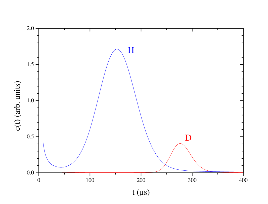
Figure 1: (Color online) Neutron Compton profiles of hydrogen and deuterium at a scattering angle of $\theta=70^{o}$ calculated considering as flight paths $L_{0}$ = 1105.5 cm and $L_{1}$ = 69 cm, assuming a gold foil analyzer of $\rm nT=4\times 10^{-5}$ barn^-1 and effective temperatures of 115.22 and 80.11 meV respectively.

IV.1 Study of the variable $y_{M}$

We will begin our discussion by examining the behavior of the $y_{M}$ variable as a function of the time of flight. In Fig. 2 we show its behavior according to Eq. (13) as a function of the incident neutron energy $E_{0}$ at different times of flight, for the case of hydrogen (M/m=0.99862) at $\theta=$70o. The behavior at the limits commented in Eq.(14) are observed. In the same figure we show the behavior of $\tilde{y}_{M}$ according to the conditions normally employed in the CA framework (Sect. II.2). The differences between both ways to define $y$ is evident: while in the exact formalism there is a whole range of possible values of $y$ at each time of flight (which is a function of $E_{0}$), in the CA there is only one value of $y$ defined at each $t$. We observe the curves $y(E_{0})$ in the exact formalism intersects the one of the CA in two points. However at each time of flight there is only one value of $y$ defined in the CA framework. Thus, only one of those two points over the exact $y$-curve has a final energy corresponding to that of the filter (4.906 eV), while the other has the same value of $y$ and $E_{0}$ but a different $E$. At 85.22 $\mu$sec, both points coincide so the curves are tangent. At times of flight greater than 85.22 $\mu$sec, this property is found in the intersection of the leftmost point between both curves, while at times lower than 85.22 $\mu$sec we find it in the rightmost intersection point.

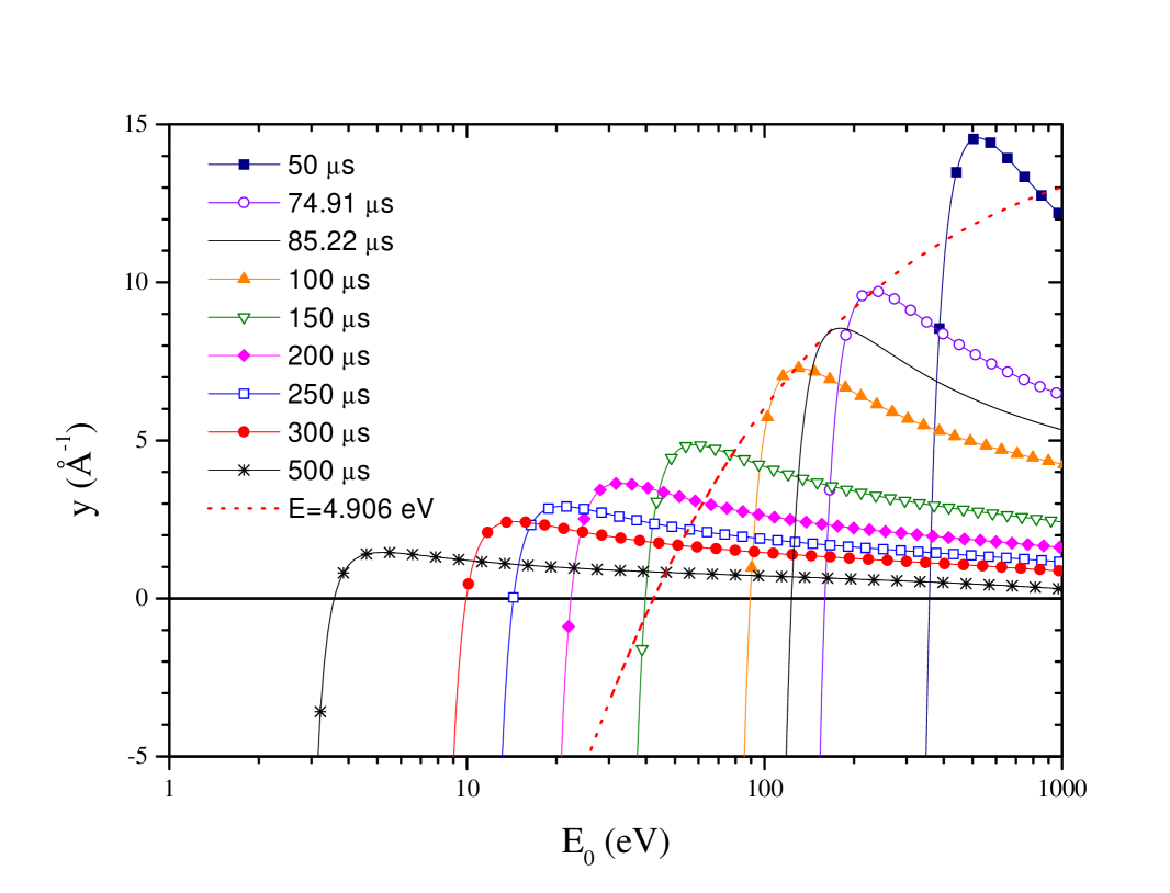
Figure 2: (Color online) The impulse $y$ as a function of the incident energy $E_{0}$ for A=0.99862. The exact calculations according to Eq. (13) at the indicated times of flight are compared with the calculation performed by assuming the final energy fixed at 4.906 eV, which is the variable $\tilde{y}$ employed in the CA framework

The behaviors observed in Fig. 2 are clarified in Fig. 3(a), where we mapped on the $(E_{0},E)$-plane the constant-$y$ and constant-$t$ curves, for the case of hydrogen. In Appendix B we show the details for the calculation of the constant $y$ curves. We also show the constant-$E$ line corresponding to main peak absorption energy of the gold analyzer (E=4.906 eV). The intersection of a constant-$t$ curve with the 4.906 eV-line defines an $E_{0}$-value with which the $y$-value in the CA framework is calculated. It can be easily shown that in this case for each constant-$t$ curve, there is one (and only one) tangent constant-$y$ curve. The geometric loci of the tangency points in the $(E_{0},E)$-plane result to be straight lines (which will be called limit lines (LL) hereafter) whose slopes can be obtained from the real positive roots of Eq. (17). Bearing in mind Eq. (III) those slopes are the squares of such roots. In this particular case of hydrogen $\displaystyle\frac{dy}{dE_{0}}\Bigg{|}_{\rm{t},\theta}=0$ has only one real root, which defines the line $E=0.021E_{0}$ as the sought geometric locus of the tangency points, which is represented in Fig. 3(b). In the representation of Fig. 2 this corresponds to the geometric locus of the maxima of the $y(E_{0})$ curves. It is worth to point out that the consequence of having one real root in Eq. (17) is that there are two branches, so $N_{R}=1$ in Eq. (20). In Fig. 3(b) we show a detail of the upper frame. The line $E=0.021E_{0}$ intersects the constant $E=4.906eV$ at a point corresponding to $t=$74.91 $\mu$sec and $y=$ 9.73 Å^-1. In consequence, in Fig. 2 the intersection between $\tilde{y}$ and the curve of 74.91 $\mu$sec occurs at its maximum. The importance of the LL resides in that it indicates the $y$ values where $f_{M}(y,t)$ presents singularities, and will be commented in the next section.

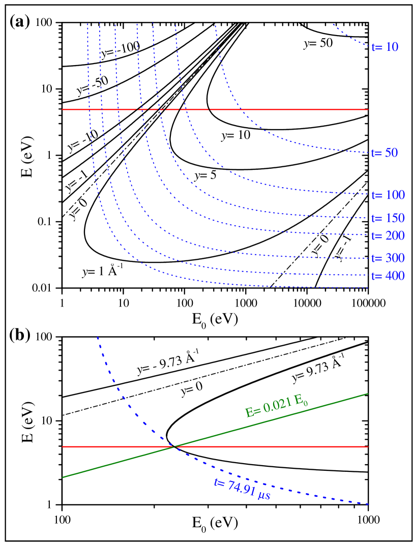
Figure 3: (Color online) (a) The full thick lines indicate the constant-$y$ curves for hydrogen at $\theta=70^{o}$ and $\ell=16.022$. $y$-values are indicated in Å^-1. In dotted lines, the curves of $t=$ constant (the indicated values are in $\mu$sec). The horizontal full line corresponds to E=4.906 eV. (b) Detail of the upper frame showing a case where a constant-$t$ and a constant-$y$ curve are tangent. The particular case of a tangency at $E$=4.906 eV was selected (see text for details).

The slope of the LLs is a function of the scattering angle and $\ell$. This is shown in Fig. 4, for $\ell=16.022$. In the case of hydrogen a LL can be defined in the whole angular range from 0o to 90o existing only one of such LLs as already mentioned. On the other hand, for deuterium there exist two real positive solutions of Eq. (17) below 39.7o and so two LLs, and for oxygen we observe the same situation at a limit angle of 24.7o.

It is also interesting to observe in Fig. 5 the representation in the $(E_{0},E)$-plane for deuterium at $\theta=$35o. In this case there exist two LLs (in accordance with Fig. 4), which are shown in the graph.

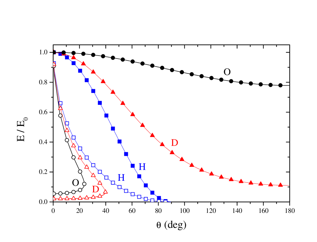
Figure 4: (Color online) The open symbols indicate value of the slopes of the straight lines corresponding to the geometric loci of the tangency points between constant-$t$ and constant-$y$ curves in the $(E,E_{0})$-plane as a function of the scattering angle, for H, D and O, with a flight-paths ratio $\ell=16.022$. Full symbols indicate the ratio $E/E_{0}$ in the cold-gas limit for H, D and O.

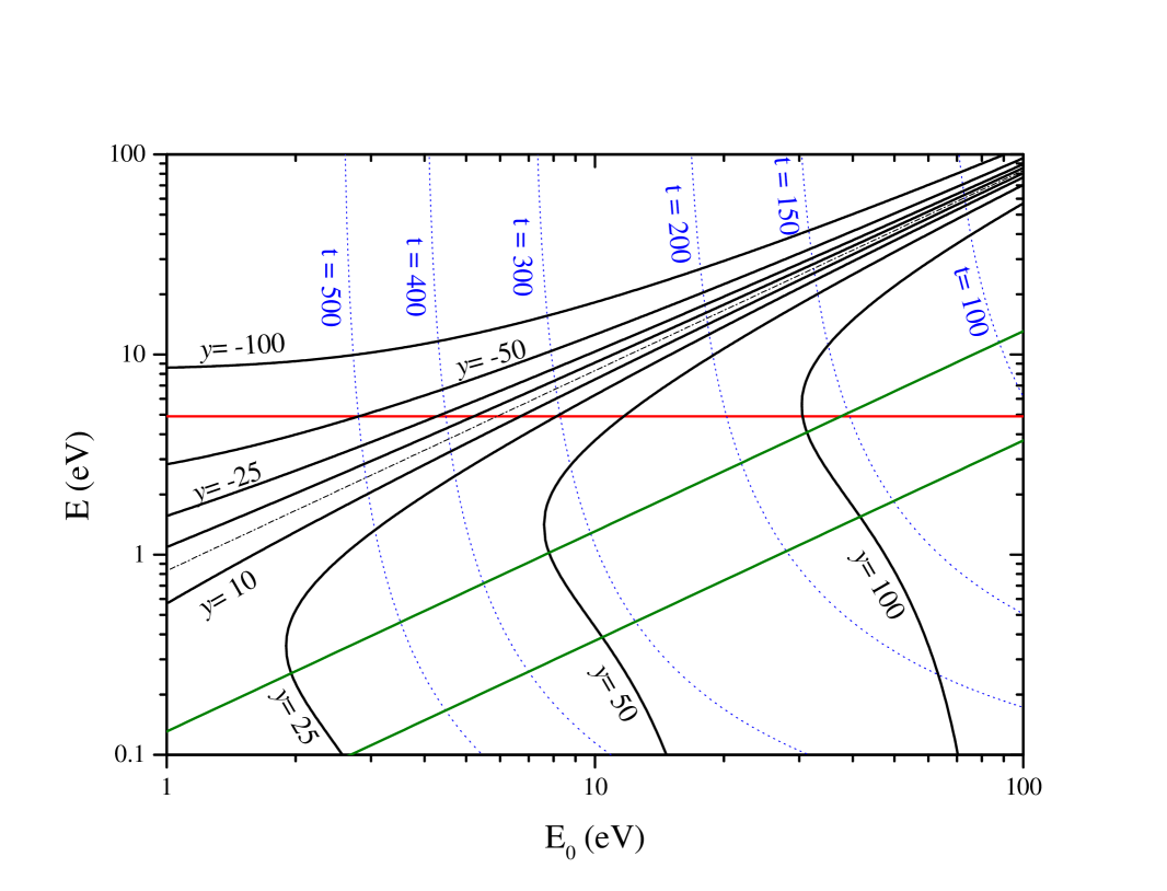
Figure 5: (Color online) The full thick lines indicate the constant-$y$ curves for deuterium at $\theta=35^{o}$ and $\ell=16.022$. $y$-values are indicated in Å^-1. In dotted lines, the curves of $t=$ constant (the indicated values are in $\mu$sec). The line corresponding to $y=$0 is shown in dash-dotted line.

IV.2 Kernel $f_{M}(y_{M},t)$

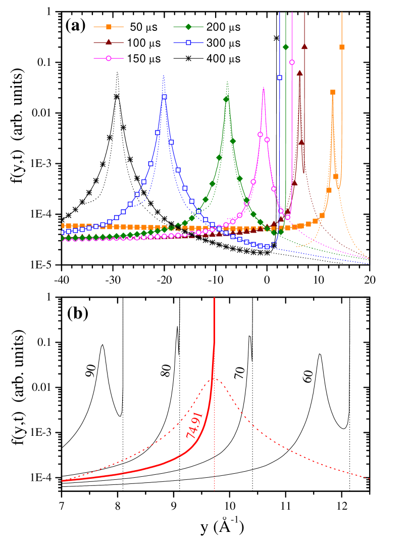
Figure 6: (Color online) (a) Full lines: $f(y,t)$ at $\theta=70^{o}$ for the indicated times of flight. Vertical dotted lines: position of the asymptotes of $f(y,t)$. Dotted lines: Resolution function times the amplitude factor $\xi(t)$, centered at the $\tilde{y}_{M}(t)$ values. See text for details. (b) Detail of the upper frame. Full thick line: $f(y,t)$ for the special case of t=74.91 $\mu$s, for which the asymptote position agrees with the value of $y$ where the resolution function times $\xi(t)$ (dotted thick line) is centered. Full thin lines: $f(y,t)$ where the values of $t$ are indicated in $\mu$sec.

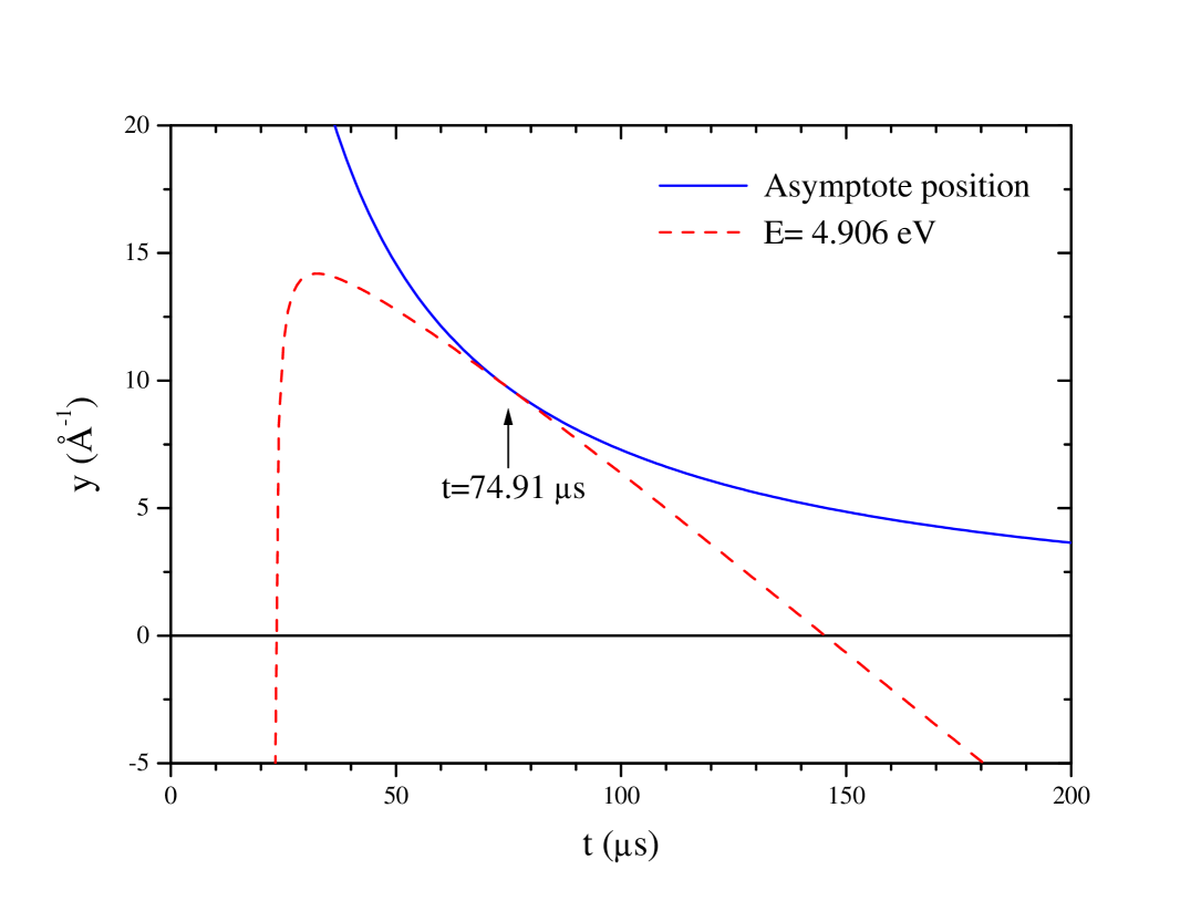
Figure 7: (Color online) Asymptote position of $f(y,t)$ as a function of the time of flight $t$, for the case of hydrogen at a scattering angle of $\theta=70^{o}$, and flight length of $L_{0}$ = 1105.5 cm and $L_{1}$ = 69 cm.

Having established the behavior of the variable $y_{M}$ we can now analyze Eq. (23). We are especially interested in examining the kernel $f_{M}(y_{M},t)$. In Fig. 6 we show its behavior in the case of scattering in hydrogen at 70o for different times of flight of interest in the Compton profile, as can be checked in Fig. 1. It is very important to notice the asymptotic behavior of $f_{M}(y_{M},t)$ at the values of $y_{M}$ defined by the LL, that is understood from the fact that the Jacobian $\displaystyle\frac{dE_{0}}{dy}\Bigg{|}_{\rm{t},\theta}\to\infty$ in Eq. (21). In the same figure we show the corresponding kernel in the CA framework expressed in the left hand side of Eq. (24), where the resolution function was calculated according to Eq(12). The maxima of both distributions are observed to be located at $\tilde{y}_{M}(t)$, i.e. the $y$ variable as defined in the CA framework. However, the asymptotes present in the exact formulation mark important differences between both formulations, which are clearly manifested at 74.91 $\mu$sec, as showed in Fig. 6(b), where the asymptote is exactly in $\tilde{y}_{M}(t)$. This effect is further illustrated in Fig. 7, where the asymptote position is shown as a function of $t$ together with $\tilde{y}_{M}(t)$. Both curves are tangent at 74.91 $\mu$sec. Alternatively, the interpretation of this point can be understood from the inspection of Fig. 3(b). In the $(E_{0},E)$-plane this point is the intersection between the LL and the $E=$4.906-eV line. On any constant-$t$ curve the maximum value of $y$ occurs in its intersection with the LL (point A), so in general this value of $y$ is greater than the one at its intersection with the constant line $E=$4.906 eV (point B). But at the precise time where both lines intersect points A and B coincide. This is manifested in Fig. 7 where the $y$ values of the asymptote position are always greater than those of the constant line $E=$4.906 eV except at the tangency point.

Besides the mentioned asymptotic behavior, there exist two other important features not described in the CA framework, viz. the main peak width and height depends on $t$, at variance with the left hand side member of Eq. (24). Similarly, those behaviors are observed in deuterium (not shown in this paper).

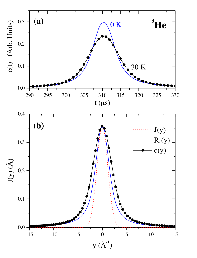
Figure 8: (Color online) (a) Neutron Compton profiles in the time of flight scale of ³He at a scattering angle of 70o, at 0K (line) and 30 K (circles). (b) The dotted line indicates the Gaussian momentum distribution $J(y)$ of ³He with a mean kinetic energy of 30 K. In full line, the resolution function calculated according to Eq.(12) and $c(t)_{T=0K}$ shown in frame (a). Circles indicate the NCP calculated at 30 K expressed as a function of the $y$ variable in the CA framework.

IV.3 Study of the mean kinetic energy

An immediate consequence of the present analysis can be found in the study of the mean kinetic energies, which is the main aim of the DINS technique. We will focus our attention to a sample constituted by an ideal gas of ³He with a mean kinetic energy of 30 K ($k_{B}T=$1.7234 meV). Such system was extensively examined in the literature Sene ; Wang ; Sokol . The NCP corresponding to this system can be obtained in the exact formalism with Eq. (20) and is shown in Fig. 8(a) (circles), which corresponds to a Gaussian distribution $J(y)$ with a full-width-at-half-maximum (FWHM) of 1.3151 Å^-1. The geometry, the filter and the efficiency are the same described at the beginning of this section. The function $J(y)$ is shown Fig. 8(b)(dotted line).

We now compare the exact formalism with the results produced in the CA framework. The resolution function can be obtained from the limit $T\to$ 0K of the NCP (shown in full line in Fig. 8(a)), and it is calculated in Eq. (12), thus obtaining the $R_{1}(y)$ shown in Fig. 8(b) (full line). The total cross section for gold employed in its calculation was taken from Ref. ENDF, . Following the procedure already described Blos1 , Eq. (10) was employed to perform a least-squares fit of a Gaussian $J(y)$ on the exact NCP, letting the area and the width of the Gaussian as free parameters. Despite being $R_{1}$ the only resolution function in the CA framework compatible with the limit at $T\to$0 K, we tested three other different resolution functions based on the customary use

CA	Mean Kinetic Energy (meV)
$R_{1}$	1.694
$R_{2}$	1.374
$R_{3}$	1.353
$R_{4}$	1.519
Exact value	1.7234

Table 1: Mean kinetic energy of ³He at 30 K obtained in the CA framework according to different resolution functions described in the text. The exact value is includes for comparison.

• $R_{2}(y)$, obtained by fitting a Lorentzian function in the energy scale PRLdeellos ; dd to the main resonance peak at 4.906 eV of the gold total cross sectionENDF , and employing Eq (12).

• $R_{3}(y)$, a Lorentzian function in the $y$ variable Timms ; Evans ; Fielding fitted to $R_{2}(y)$. The resulting FWHM is 3.292 Å^-1.

• $R_{4}(y)$, a Lorentzian function in the $y$ variable Timms ; Evans ; Fielding fitted to $R_{1}(y)$. The resulting FWHM is 3.170 Å^-1.

In table 1 we show the resulting effective temperatures, compared with the exact value, used as input to generate $J(y)$. It is worth to remark that the different choices of $R(y)$ produces large variations in the effective temperature, even when the FWHM has no such large variations. For example, the change in FWHM from $R_{3}$ to $R_{4}$ is 3.7 % and the resulting mean kinetic energies differ in 12.3 %. The reason for such a large change, was reported in Ref. Blos1, : at low temperatures the shape of the observed NCP is determined mainly by the filter, so any imperfection in the description of the filter effects will affect significantly the obtained mean kinetic energy.

V Conclusions

In this paper we developed the exact formalism that describes the NCPs obtained from DINS experiments in terms of an integral equation in the variable $y$ that involves a kernel dependent on the experimental setup parameters. For its calculation, a precise knowledge of the detectors efficiency, the filter total cross section and the incident neutron spectrum in a wide range of energies is required. As a result, we obtained a Volterra equation of the first kind that allows to obtain the desired momentum distribution $J(y)$ by means of numerical methods.

A significant part of this paper was devoted to the study of the variable $y$, that in the exact formalism here presented has a definition that differs significantly from that employed in the CA framework. The physical significance of this variable is the projection of the initial impulse of the target nuclei over the direction of the momentum transfer vector $\bm{q}$. In DINS data processing procedures the passage from $t$ to $y$ is customarily calculated taking a fixed final energy, and thus it has a single well-defined value for each time channel. In this paper it was calculated exactly. The importance of knowing the exact mapping of the variable $y$ in the $(E_{0},E)$-plane can be referred to our recent study on the neutron final energy distributions in DINS experiments FinalE . In that work we found that such distributions are far more complex than considering a single final energy, and depends on the time channel and the dynamics of the scattering species. We showed the constant-$y$ curves on the $(E_{0},E)$-plane for hydrogen and deuterium at a particular scattering angle and ratio of flight paths, which served to illustrate its behavior, and developed its general expressions. A noticeable particularity of the $y$ variable in the exact treatment that we present in this paper, is that it can have local extrema as a function of $E_{0}$ for a given time of flight as shown in Fig. 2, which define straight lines in the $(E_{0},E)$-plane (LL). This causes singularities in the Jacobian $dE_{0}/dy_{M}$ which affect the kernel $f_{M}(y_{M},t)$. For example in the analyzed case of hydrogen, values of $y$ greater that that those defined by the LL are not physically allowed.

In past publications Blos1 ; Blos2 we showed that CA can not be deduced from the exact expression. In this paper we again showed that the CA formalism is incompatible with the exact one, and that the basis of the difference between both formalisms resides in the integration kernels. Thus, the resolution function must be replaced by a kernel that depends on $t$. In Fig. 6 we show explicitly the differences between the exact kernel and the commonly accepted resolution function. Besides the clearly observed differences in shape, it is notable the appearance of the above mentioned singularities. In the particular case analyzed in this paper these discrepancies are particularly noticeable at 74.91 $\mu$sec, where the singularity occurs exactly at the value of $y$ where the maximum of the resolution function is centered, i.e. at $y=\tilde{y}_{M}(t)$.

So far, we have focussed our discussion on the differences between the kernel $f_{M}(y_{M},t)$ and the resolution function, without making any reference to the momentum distribution of the sample $J_{M}(y_{M})$. As a first exam on the interrelation between $f_{M}(y_{M},t)$ and $J_{M}(y_{M})$ it is helpful to check to what extent the singularity can affect significant parts of the integrand (20). To this end we will compare the ratio $E/E_{0}$ where the singularities appear (defined by the slope of the LL) with the same ratio for the scattering on a sample defined by an ideal gas at $T=$0K, i.e. Blos1

$$\frac{E}{E_{0}}=\left(\frac{\cos\theta+\sqrt{\cos^{2}\theta+(A-1)(A+1)}}{A+1}\right)^{2}.$$ (25)

Eq. (25) defines also the most probable energy ratio in the case of a sample at finite temperature. In Fig. 4 we show in open symbols the ratio $E/E_{0}$ of the LL for H, D and O, and in full symbols that corresponding to Eq. (25), as a function of the scattering angle. We observe that for this particular value of $\ell$ the singularities do not appear significantly near the main peak. However, due to the thermal motion (described by the shape of $J(y)$) the singularities affect the description of the tails of NCPs.

The present formalism was formulated regardless of the function $J(y)$. Although in this paper the case of an isotropic sample was examined, all the considerations we developed are applicable also for the case of anisotropic samples. It is also worth to notice that although in most of the significant cases concerning the study of Condensed Matter the function $J(y)$ is closely represented by a Gaussian shape Mayers90 , this function could represent an anisotropic momentum distribution, not centered in $y=0$ like in the case of particles flowing in a preferential direction. With regard to the analysis of experiments where the sample can be represented by the usual Gaussian distributions, it must be emphasized that the effects of the singularities will normally be smoothed out in the NCP, i.e. the experimentally accessible magnitude. However, the differences between the exact formalism and the CA in the description of the NCP are clearly manifested, as accounted in detail in Ref. Blos1, , so we will briefly summarize them here. A comparison of the results produced by Eq. (10) in the calculation of the NCPs, with the exact formalism represented either by Eqs. (1) or (19) (both formulations are equivalent, since they differ only in the integration variable), reveal that the CA is defective in the description of

• the peak areas,

• the peak centroids,

• the peak widths,

being the case of light scatterers at low temperatures the most sensitive ones to these imperfections. In this case the widths of the momentum distribution function $J(y)$, and the resolution function $R(y)$ becomes comparable, and thus the consequences of the differences between $R(y)$ and the exact kernel is more clearly manifested on the NCPs. Thus, the obtainment of peak areas and effective temperatures is significantly affected because of the use of the CA. The analysis shown in Sect. IV.3, clearly reflects this assertion, and the inadequacy to employ resolution functions (either theoretically or experimentally defined) that due to the approximate nature of the CA has an unavoidable degree of ambiguity in its definition.

We wish to conclude this paper giving a schematic outline of the procedure we recommend to use to the experimentalists in the DINS field. For the measurement of an impulse distribution function it is necessary to characterize different parameters of the experimental configuration.

1. The incident neutron energy spectrum can be determined by a measurement with a detector of well-characterized efficiency placed on the direct beam.

2. The efficiency of the detectors bank can be characterized using a heavy target (like Pb or Bi) at the sample position (with the filter out of the scattered neutron path).

3. The effective filter thickness can be measured with a lead target, employing the method ‘filter in - filter out’, and fitting it as a parameter in Eq. (1). Alternatively, a transmission experiment can be performed on the direct beam. In the process, the full total cross section of the filter is needed. A wide variety of cross sections can be found v. gr. in Ref. ENDF, .

4. Experimental data must be corrected by multiple scattering and attenuation effects, using Monte Carlo procedures like those described in Refs. MonteCarloEllos, and MonteCarloNuestro, .

5. From the steps 1 to 3, which aim to know the kernel $f(y,t)$, and step 4 which corrects for finite sample effects, we obtain the necessary elements to state Eq. (20), that can be solved either by numerical means or by fitting parameters if we have a previous knowledge of the function $J(y)$. In this last instance the fitting process can be made also directly on the $t$ scale employing Eq. (1) without changing the integration variable from $E_{0}$ to $y$.

Finally, let us mention that the present formalism is also applicable to the method of double differences recently presented dd , which consists in employing two filters of different thicknesses. The use of the formalism presented in our paper will be most beneficial for the users community of these DINS techniques.

Appendix A Derivation of $dy/dE_{0}$

From the definition of the $y$ of Eq. (7) we have

$$\frac{dy}{dE_{0}}\Big{|}_{t} = \frac{\partial y}{\partial q}\frac{dq}{dE_{0}}\Big{|}_{t}+\frac{\partial y}{\partial\omega}\frac{d\omega}{dE_{0}}\Big{|}_{t}$$ (26)

$$= \left(\frac{-M\omega}{q^{2}}-\frac{\hbar}{2}\right)\frac{dq}{dE_{0}}\Big{|}_{t}+\frac{M}{q}\frac{d\omega}{dE_{0}}\Big{|}_{t}$$

So, we need to calculate the derivatives of $q$ and $\omega$ with respect to $E_{0}$ at constant $t$. Form Eq. (4) we have

$$\frac{d\omega}{dE_{0}}\Big{|}_{t}=\frac{1}{\hbar}\left(1-\frac{dE}{dE_{0}}\Big{|}_{t}\right)$$ (27)

From the kinematic condition (2) we have

$$\frac{dE}{dE_{0}}\Big{|}_{t}=-\frac{L_{0}}{L_{1}}{\left(\frac{E}{E_{0}}\right)}^{3/2}$$ (28)

Replacing Eq.(28) in Eq.(27) we have

$$\frac{d\omega}{dE_{0}}\Big{|}_{t}=\frac{1}{\hbar}\left(1+\frac{L_{0}}{L_{1}}\left(\frac{E}{E_{0}}\right)^{3/2}\right)$$ (29)

On the other hand, deriving the definition of $q$ presented in Eq. (5) we have

$$\frac{dq}{dE_{0}}\Big{|}_{t}=\frac{\partial q}{\partial E_{0}}\Big{|}_{t}+\frac{\partial q}{\partial E}\frac{\partial E}{\partial E_{0}}\Big{|}_{t}.$$ (30)

Then

$$\frac{dq}{dE_{0}}\Big{|}_{t}\!=\!\frac{m}{\hbar^{2}q}\left[1-\frac{L_{0}}{L_{1}}{\left(\frac{E}{E_{0}}\right)}^{3/2}\!\!+\!\left(\frac{L_{0}}{L_{1}}\frac{E}{E_{0}}\!-\!\sqrt{\frac{E}{E_{0}}}\right)\cos\theta\right]$$ (31)

where we have employed Eq.(28). Finally, replacing Eq. (29) and Eq. (31) in Eq. (26) we obtain Eq. (15).

Appendix B Derivation of $E(E_{0},y)$

From the Eq. (13) for $y$ (which is in terms of $E$ and $E_{0}$), we want to solve it for $E$, considering $y$ and $E_{0}$ as fixed input values. Defining the variables

$$\left\{\begin{array}[]{lll}x&=&\sqrt{E}\\ \alpha&=&\frac{\displaystyle M^{2}}{\displaystyle 2my^{2}}\\ \mu&=&\frac{\displaystyle m}{\displaystyle M}\\ \end{array}\right.,$$

after some algebra Eq. (13) can be transformed to a fourth-order polynomial in $x$, with real coefficients

$$\mathop{\sum}_{i=0}^{4}b_{i}{x^{i}}=0$$ (32)

where

$$b_{0} = \left[\alpha\left(1-\mu\right)^{2}E_{0}-1\right]E_{0}$$

$$b_{1} = 2\left[1+2\alpha\left(\mu-\mu^{2}\right)E_{0}\right]\sqrt{E_{0}}\cos\theta$$

$$b_{2} = -1-2\alpha\left[1-\mu^{2}-2\mu^{2}{\cos}^{2}\theta\right]E_{0}$$ (33)

$$b_{3} = -4{\alpha}{\mu}\left(1+\mu\right)\sqrt{E_{0}}\cos\theta$$

$$b_{4} = \alpha\left(1+\mu\right)^{2}.$$

Therefore, the real positive roots of Eq. (32) define the values of $E(E_{0},y)$, which define the $y$-constant curves represented in Figs. 3 and 5.

References

- (1) V.F. Sears, Physical Review B, 30, 44 (1984).
- (2) M. Breidenbach et al., Phys. Rev. Lett. 23, 935-939 (1969).
- (3) R. Holt, J. Mayers and A. Taylor in Momentum Distributions, edited by R.N. Silver and P.E. Sokol (Plenum, New York, 1989) p. 295.
- (4) P.C. Hohenberg and P.M. Platzmann, Phys. Rev. 152, 198 (1966).
- (5) A.C. Evans, J. Mayers, D.N. Timms, M.J. Cooper, Z. Naturforsch. 48a, 425-432 (1993).
- (6) D. N. Timms, A. C. Evans, M. Boninsegni, D. M. Ceperley, J. Mayers and R. O. Simmons, J. Phys.: Condens. Matter 8, 6665 (1996).
- (7) R. Senesi et al., Physica B 200, 276 (2000).
- (8) A. L. Fielding, J. Mayers, Nuclear Instruments and Methods in Physics Research A 480, 680 (2002).
- (9) V. F. Sears, Phys. Rev. A 5, 452 (1971).
- (10) V. F. Sears, Phys. Rev. A 7, 340 (1973).
- (11) P.M. Platzmann, in Momentum Distributions, edited by R.N. Silver and P.E. Sokol (Plenum, New York, 1989) p. 249.
- (12) R. Newton, Scattering Teory of Waves and Particles, (Springer, Berlin, 1981).
- (13) V.F. Sears, Physical Review 185, 200 (1969).
- (14) A. D. B. Woods and V.F. Sears, Phys. Rev. Lett. 39, 415 (1977).
- (15) J.J. Weinstein and J.W. Negele, Phys. Rev. Lett. 49, 1016 (1982).
- (16) J. Mayers, C. Andreani and G. Baciocco, Phys. Rev. B 39, 2022 (1989).
- (17) J. Mayers, Physical Review B, 41, 41, (1990).
- (18) J. Mayers and A.C. Evans, Rutherford Appleton Laboratory Technical Report, RAL-TR-96-067 (1996).
- (19) J. Mayers, A. L. Fielding, R. Senesi, Nucl. Instr. Meth. Phys. Res. A 481, 454 (2002).
- (20) J. J. Blostein, J. Dawidowski and J.R. Granada, Physica B. 304, 357-367, (2001).
- (21) J. J. Blostein, J. Dawidowski and J.R. Granada, Physica B, 334, 257 (2003).
- (22) C. A. Chatzidimitriou-Dreismann, T. Abdul-Redah, R.M.F. Streffer, and J. Mayers, Phys.Rev.Lett. 79, 2839, (1997).
- (23) J. J. Blostein, J. Dawidowski, S. A. Ibáñez and J. R. Granada, Phys. Rev. Lett. 90, 105302 (2003).
- (24) R.A. Cowley, J. Phys.: Condens. Matter 15 (2003) 41434152
- (25) D. Colognesi, Physica B (in press, available online) (2003)
- (26) J. J. Blostein, J. Dawidowski and J.R. Granada, Nucl. Instr. and Meth., in press (2003).
- (27) ENDF/B-VI, IAEA Nuclear Data Section, 1997.
- (28) J. Dawidowski, J.J. Blostein and J.R. Granada, in: M.R. Johnson, G.J. Kearley, H.G. Büttner (Eds.) Neutron and Numerical Methods, American Institute of Physics, New York, (1999), p. 37.
- (29) R. Senesi, C. Andreani, D. Colognesi, A. Cunsolo, M. Nardone, Phys. Rev. Lett., 86, 4584 (2001).
- (30) Y. Wang and P.E. Sokol, Phys. Rev. Lett., 72, 1040 (1994).
- (31) P.E. Sokol, K. Sköld, D.L. Price and R. Kleb, Phys. Rev. Lett., 54, 909, (1985).
- (32) C. Andreani, D. Colognesi, E. Degiorgi, A. Filabozzi, M. Nardone, E. Pace, A. Pietropaolo and R. Senesi, Nucl. Instr. Meth. A 497, 535 (2003).