Open-source software for generating electrocardiogram signals

Abstract

ECGSYN, a dynamical model that faithfully reproduces the main features of the human electrocardiogram (ECG), including heart rate variability, RR intervals and QT intervals is presented. Details of the underlying algorithm and an open-source software implementation in Matlab, C and Java are described. An example of how this model will facilitate comparisons of signal processing techniques is provided.

1 Introduction

The field of biomedical signal processing has given rise to a number of techniques for assisting physicians with their everyday tasks of diagnosing and monitoring medical disorders. Analysis of the electrocardiogram (ECG) provides a quantitative description of the heart’s electrical activity and is routinely used in hospitals as a tool for identifying cardiac disorders.

A large variety of signal processing techniques have been employed for filtering the raw ECG signal prior to feature extraction and diagnosis of medical disorders. A typical ECG is invariably corrupted by (i) electrical interference from surrounding equipment (e.g. effect of the electrical mains supply), (ii) measurement (or electrode contact) noise, (iii) electromyographic (muscle contraction), (iv) movement artefacts, (v) baseline drift and respiratory artefacts and (vi) instrumentation noise (such as artefacts from the analogue to digital conversion process) (?).

Many techniques may be employed for filtering and removing noise from the raw ECG signal, such as wavelet decomposition (?), Principal Component Analysis (PCA) (?), Independent Component Analysis (ICA) (?), nonlinear noise reduction (?) and traditional Wiener methods. The ECG forms the basis of a wide range of medical studies, including the investigation of heart rate variability, respiration and QT dispersion (?). The utility of these medical indicators relies on signal processing techniques for detecting R-peaks (?), deriving heart rate and respiratory rate (?), and measuring QT-intervals (?).

Despite the numerous techniques that may be found in the literature and those that are now freely available on the Internet (?), it remains extremely difficult to evaluate and contrast their performance. The recent proliferation of biomedical databases, such as Physiobank (?), provides a common setting for comparing techniques and approaches. While this availability of real biomedical recordings has and will continue to advance the pace of research, the lack of internationally agreed upon benchmarks means that it is impossible to compare competing signal processing techniques. The definition of such benchmarks is hindered by the fact that the true underlying dynamics of a real ECG can never be known. This void in the field of biomedical research calls for a gold standard, where an ECG with well-understood dynamics and known characteristics is made freely available.

The model presented here, known as ECGSYN (synthetic electrocardiogram), is motivated by the need to evaluate and quantify the performance of the above signal processing techniques on ECG signals with known characteristics. While the Physionet web-site (?) already contains a synthetic ECG generator (?), this is not intended to be highly realistic. The model and its underlying algorithm described in detail in this paper is capable of producing extremely realistic ECG signals with complete flexibility over the choice of parameters that govern the structure of these ECG signals in the temporal and spectral domains. In addition, the average morphology of the ECG may be specified. In order to facilitate the use of ECGSYN, software has been made freely available as both Matlab and C code . Furthermore, users can employ ECGSYN over the Internet using a Java applet, which provides a means of downloading an ECG signal with characteristics selected from a graphical user interface.

2 Background

The average heart rate is calculated by first measuring the time interval, denoted RR interval, between two consecutive R peaks (Fig. 1), taking the average reciprocal of this value over a fixed window (usually 15, 30 or 60 seconds) and then scaling to units of beats per minute (bpm). A time series of RR intervals is often referred to as an RR tachogram and the variation in this time series is governed by the balance between the sympathetic (fight and flight) and parasympathetic (rest and digest) branches of the central nervous system, known as the sympathovagal balance. In general, innervation of the fast acting parasympathetic branch decreases heart rate, whereas the (more slowly acting) sympathetic branch increases heart rate. This RR tachogram can therefore be used to estimate the effect of both these branches. A spectral analysis of the RR tachogram is usually divided into main frequency bands, known as the low-frequency (LF) band (0.04 to 0.15 Hz) and high-frequency (HF) band (0.15 to 0.4 Hz) (?). Sympathetic tone is believed to affect the LF component whereas both sympathetic and parasympathetic activity influence the HF component (?). The ratio of the power contained in the LF and HF components has been used as a measure of the sympathovagal balance (?, ?).

The structure of the power spectrum of the RR tachogram tends to vary from person to person with a number of spectral peaks associated with particular biological mechanisms (?, ?). While the correspondence between these mechanisms and the positions of spectral peaks are strongly debated, there are two peaks which usually appear in most subjects. These are due to Respiratory Sinus Arrhythmia (RSA) (?, ?) caused by parasympathetic activity which is synchronous with the respiratory cycle and Mayer waves caused by oscillations in the blood pressure waves (?). RSA usually gives rise to a peak in the HF region around 0.25 Hz, corresponding to 15 breaths per minute, whereas the Mayer waves cause a peak around 0.1 Hz.

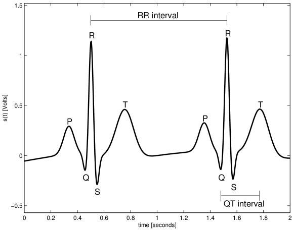
Figure 1: Two seconds of synthetic ECG reflecting the electrical activity in the heart during two beats. Morphology is shown by five extrema P,Q,R,S and T. Time intervals corresponding to the RR interval and the QT interval are also indicated.

3 Method

The dynamical model, ECGSYN, employed for generating the synthetic ECG is composed of two parts. Firstly, an internal time series with internal sampling frequency $f_{\rm int}$ is produced to incorporate a specific mean heart rate, standard deviation and spectral characteristics corresponding to a real RR tachogram. Secondly, the average morphology of the ECG is produced by specifying the locations and heights of the peaks that occur during each heart beat. A flow chart of the processes in ECGSYN for producing the ECG is shown in Fig. 2.

Figure 2: ECGSYN flow chart describing the procedure for specifying the temporal and spectral description of the RR tachogram and ECG morphology.

The spectral characteristics of the RR tachogram, including both RSA and Mayer waves, are replicated by specifying a bi-modal spectrum composed of the sum of two Gaussian functions,

$$S(f)=\frac{\sigma_{1}^{2}}{\sqrt{2\pi c_{1}^{2}}}\exp\left(\frac{(f-f_{1})^{2}}{2c_{1}^{2}}\right)+\frac{\sigma_{2}^{2}}{\sqrt{2\pi c_{2}^{2}}}\exp\left(\frac{(f-f_{2})^{2}}{2c_{2}^{2}}\right),$$ (1)

with means $f_{1},f_{2}$ and standard deviations $c_{1},c_{2}$. Power in the LF and HF bands are given by $\sigma_{1}^{2}$ and $\sigma_{2}^{2}$ respectively whereas the variance equals the total area $\sigma^{2}=\sigma^{2}_{1}+\sigma^{2}_{2}$, yielding an LF/HF ratio of $\sigma^{2}_{1}/\sigma^{2}_{2}$.

A time series $T(t)$ with power spectrum $S(f)$ is generated by taking the inverse Fourier transform of a sequence of complex numbers with amplitudes $\sqrt{S(f)}$ and phases which are randomly distributed between 0 and $2\pi$. By multiplying this time series by an appropriate scaling constant and adding an offset value, the resulting time series can be given any required mean and standard deviation. Different realisations of the random phases may be specified by varying the seed of the random number generator. In this way, many different time series $T(t)$ may be generated with the same temporal and spectral properties.

The ECG traces a quasi-periodic waveform with each beat of the heart, with the morphology of each cycle labeled by its peaks and troughs, P, Q, R, S and T, as shown in Fig. 1. This quasi-periodicity can be reproduced by constructing a dynamical model containing an attracting limit cycle; each heart beat corresponds to one revolution around this limit cycle, which lies in the $(x,y)$-plane as shown in Fig. 3. The morphology of the ECG is created by using a series of exponentials to force the trajectory to trace out the PQRST-waveform in the $z$-direction. A series of five angles, ($\theta_{P}$, $\theta_{Q}$, $\theta_{R}$, $\theta_{S}$, $\theta_{T}$), are used to specify the extrema of the peaks (P,Q,R,S,T) respectively.

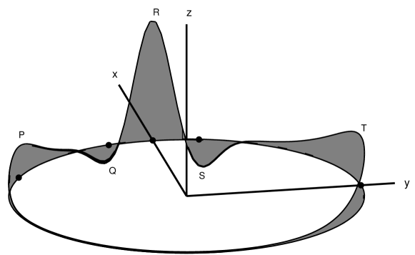
Figure 3: Three-dimensional state space of the dynamical system given by (2) showing motion around the limit cycle in the horizontal $(x,y)$-plane. The vertical $z$-component provides the synthetic ECG signal with a morphology that is defined by the five extrema P,Q,R,S and T.

The dynamical equations of motion are given by three ordinary differential equations (?),

$${\dot{x}} = \alpha x-\omega y,$$

$${\dot{y}} = \alpha y+\omega x,$$

$${\dot{z}} = -\!\!\!\!\!\!\sum_{i\in\{P,Q,R,S,T\}}\!\!\!\!\!\!a_{i}\Delta\theta_{i}\exp(-\Delta\theta_{i}^{2}/2b_{i}^{2})-(z-z_{0}),$$ (2)

where $\alpha=1-\sqrt{x^{2}+y^{2}}$, $\Delta\theta_{i}=(\theta-\theta_{i})\ {\rm mod}\ 2\pi$, $\theta={\rm atan2}(y,x)$ and $\omega$ is the angular velocity of the trajectory as it moves around the limit cycle. The coefficients $a_{i}$ govern the magnitude of the peaks whereas the $b_{i}$ define the width (time duration) of each peak. Baseline wander may be introduced by coupling the baseline value $z_{0}$ in (2) to the respiratory frequency $f_{2}$ in (1) using $z_{0}(t)=A\sin(2\pi f_{2}t)$. The output synthetic ECG signal, $s(t)$, is the vertical component of the three-dimensional dynamical system in (2): $s(t)=z(t)$.

Having calculated the internal RR tachogram expressed by the time series $T(t)$ with power spectrum $S(f)$ given by (1), this can then be used to drive the dynamical model (2) so that the resulting RR intervals will have the same power spectrum as that given by $S(f)$. Starting from the auxiliary time $t_{n}$, with angle $\theta=\theta_{R}$, the time interval $T(t_{n})$ is used to calculate an angular frequency $\Omega_{n}=\frac{2\pi}{T(t_{n})}$. This particular angular frequency, $\Omega_{n}$, is used to specify the dynamics until the angle $\theta$ reaches $\theta_{R}$ again, whereby a complete revolution (one heart beat) has taken place. For the next revolution, the time is updated, $t_{n+1}=t_{n}+T(t_{n})$, and the next angular frequency, $\Omega_{n+1}=\frac{2\pi}{T(t_{n+1})}$, is used to drive the trajectory around the limit cycle. In this way, the internally generated beat-to-beat time series, $T(t)$, can be used to generate an ECG with associated RR intervals that have the same spectral characteristics. The angular frequency $\omega(t)$ in (2) is specified using the beat-to-beat values $\Omega_{n}$ obtained from the internally generated RR tachogram:

$$\omega(t)=\Omega_{n},\ \ \ \ \ \ t_{n}\leq t<t_{n+1}.$$ (3)

Given these beat-to-beat values of the angular frequency $\omega$, the equations of motion in (2) are integrated using a fourth-order Runge-Kutta method (?). The time series $T(t)$ used for defining the values of $\Omega_{n}$ has a high sampling frequency of $f_{\rm int}$, which is effectively the step size of the integration. The final output ECG signal is then down-sampled to $f_{\rm ecg}$ if $f_{\rm int}>f_{\rm ecg}$ by a factor $\frac{f_{\rm int}}{f_{\rm ecg}}$ to generate an ECG at the requested sampling frequency. For simplicity, $f_{\rm int}$ is taken as an integer multiple of $f_{\rm ecg}$ and anti-aliasing filtering is therefore not required if $f_{\rm ecg}$ is chosen to be sufficiently high.

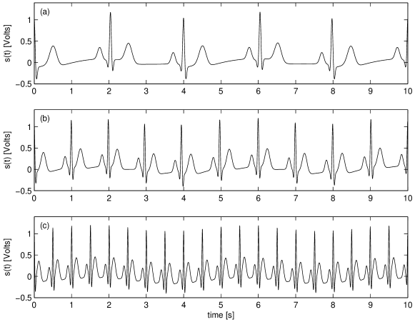
Figure 4: Synthetic ECG signals for different mean heart rates: (a) 30 bpm, (b) 60 bpm and (c) 120 bpm.

The size of the mean heart rate affects the shape of the ECG morphology. An analysis of real ECG signals for different heart rates shows that the intervals between the extrema vary by different amounts; in particular the QRS width decreases with increasing heart rate. This is as one would expect; when sympathetic tone increases the conduction velocity across the ventricles increases, together with an augmented heart rate. The time for ventricular depolarisation (represented by the QRS complex of the ECG) is therefore shorter. These changes are replicated by modifying the width of the exponentials in (2) and also the positions of the angles $\theta$. This is achieved by using a heart rate dependent factor $\alpha=\sqrt{h_{\rm mean}/60}$ where $h_{\rm mean}$ is the mean heart rate expressed in units of bpm (see Table 1).

Operation of ECGSYN, composed of the spectral characteristics given by (1) and the time domain dynamics in (2), requires the selection of the list of parameters given in Tables 1 and 2.

Table 1: Morphological parameters of the ECG model with modulation factor $\alpha=\sqrt{h_{\rm mean}/60}$.

• Index (i)	P	Q	R	S	T
  Time (secs)	-0.2	-0.05	0	0.05	0.3
  $\theta_{i}$ (radians)	$-\frac{1}{3}\pi\sqrt{\alpha}$	$-\frac{1}{12}\pi\alpha$	0	$\frac{1}{12}\pi\alpha$	$\frac{1}{2}\pi$
  $a_{i}$	1.2	-5.0	30.0	-7.5	0.75
  $b_{i}$	0.25$\alpha$	0.1$\alpha$	0.1$\alpha$	0.1$\alpha$	0.4$\alpha$

Table 2: Temporal and spectral parameters of the ECG model

• Description	Notation	Default values
  Approximate number of heart beats	$N$	256
  ECG sampling frequency	$f_{\rm ecg}$	256 Hz
  Internal sampling frequency	$f_{\rm int}$	512 Hz
  Amplitude of additive uniform noise	$A$	0.1 mV
  Heart rate mean	$h_{\rm mean}$	60 bpm
  Heart rate standard deviation.	$h_{\rm std}$	1 bpm
  Low frequency	$f_{1}$	0.1 Hz
  High frequency	$f_{2}$	0.25 Hz
  Low frequency standard deviation	$c_{1}$	0.1 Hz
  High frequency standard deviation	$c_{2}$	0.1 Hz
  LF/HF ratio	$\gamma$	0.5

4 Results

The synthetic ECG provides a realistic signal for a range of heart rates. Figure 4 illustrates examples of the synthetic ECG for three different heart rates; 30 bpm, 60 bpm, and 120 bpm. Notice that the PR, QT and QRS widths all shorten with increasing heart rate. It is important to note that the nonlinear relationship between the morphology modulation factor $\alpha$ and mean heart rate $h_{\rm mean}$ limits the contraction of the overall PQRST morphology relative to the refractory period (the minimum amount of time in which depolarisation and repolarisation of the cardiac muscle can occur).

The ability of ECGSYN to generate ECG signals with known spectral characteristics provides a means of testing the effect of varying the ECG sampling frequency $f_{\rm ecg}$ on the estimation of heart rate variability (HRV) metrics. Figure 5 illustrates the increase in estimation accuracy of a HRV metric, the LF/HF ratio, with increasing $f_{\rm ecg}$. The error bars represent one standard deviation on either side of the means (dots) of each 1000 Montecarlo runs. The true input LF/HF ratio was 0.5 as shown by the horizontal line. The synthetic ECG signals had a mean heart rate of 60 bpm and a standard deviation of 3 bpm. The method used for estimating the LF/HF ratio, the Lomb periodogram, introduces negligible variance into the estimate (?), and therefore the downward bias of the estimates can be considered due to $f_{\rm ecg}$ being too low. Note that below 512 Hz, the LF/HF ratio is considerably underestimated. This is consistent with studies performed on real data (?).

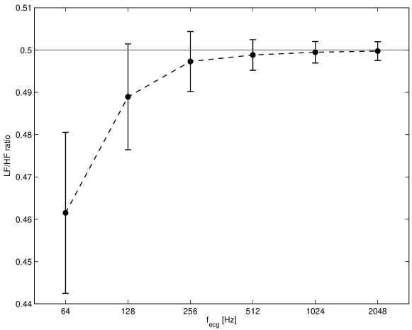
Figure 5: LF/HF ratio estimates computed from synthetic ECG signals for a range of sampling frequencies using an input LF/HF ratio of 0.5 (horizontal line). The distribution of estimates is shown by the mean (dot) and plus/minus one standard deviation error bars. The simulations used 100 realisations of noise-free synthetic ECG signals with a mean heart rate of 60 bpm and standard deviation of 3 bpm.

5 Discussion

A dynamical model known as ECGSYN has been presented that generates realistic synthetic ECG signals. The user can specify both the temporal and spectral characteristics of the ECG. In addition, the average morphology of the ECG may be input into the algorithm. Open-source software for the algorithm underlying ECGSYN is freely available in both Matlab and C. A Java applet facilitates the generation of ECG signals over the Internet with characteristics selected using a graphical user interface.

By examining the statistical properties of artificially generated ECG signals, it has been shown that estimates of HRV using the LF/HF ratio depend on the sampling frequency, $f_{\rm ecg}$, of the ECG. Small values of $f_{\rm ecg}$ gives rise to ECG signals which lead to underestimated LF/HF ratios. This provides a basis for the low sample frequency problem in HRV studies (?). In addition, these results provide a guide for physicians when selecting the sampling frequency of the ECG based on the required accuracy of the HRV metrics.

The availability of ECGSYN through open-source software and the ability to generate collections of ECG signals with carefully controlled and a priori known characteristics will allow biomedical researchers to test and provide operation statistics for new signal processing techniques. This will enable physicians to compare and evaluate different techniques and to select those that best suit their requirements.

References

References

- [1]
- [2] [] Abboud S & Barnea O 1995 Computers in Cardiology pp. 461–463.
- [3]
- [4] [] Clifford G D 1998 Signal Processing Methods for Heart Rate Variability PhD thesis University of Oxford.
- [5]
- [6] [] Davey P 1999 Heart 82, 183–186.
- [7]
- [8] [] De Boer R W, Karemaker J M & Strackee J 1987 Am. J. Physiol. 253, 680–689.
- [9]
- [10] [] Friesen G M, Jannett T C, Jadallah M A, Yates S L, Quint S R & Nagle H T 1990 IEEE Trans. Biomed. Eng. 37(1), 85–98.
- [11]
-
[12]
[]
Goldberger A L, Amaral L A N, Glass L, Hausdorff J M, Ivanov P C, Mark R G,
Mietus J E, Moody G B, Peng C K & Stanley H E 2000 Circulations 101(23), e215–e220.
*#1 - [13]
- [14] [] Hales S 1733 Statical Essays II, Haemastaticks Innings and Manby London.
- [15]
- [16] [] Ludwig C 1847 Arch. Anat. Physiol. 13, 242–302.
- [17]
- [18] [] Malik M & Camm A J 1995 Heart Rate Variability Futura Publishing Armonk, NY.
- [19]
- [20] [] McSharry P E, Clifford G, Tarassenko L & Smith L A 2002 Computers in Cardiology 29, 225–228.
- [21]
-
[22]
[]
McSharry P E, Clifford G, Tarassenko L & Smith L A 2003 IEEE
Trans. Biomed. Eng. 50(3), 289–294.
*#1 - [23]
- [24] [] Moody G B, Mark R G, Zoccola A & Mantero S 1985 Computers in Cardiology 12, 113–116.
- [25]
- [26] [] Nikolaev N, Nkolov Z, Gotchev A & Egiazarian K 2000 in ‘Proc. of ICASSP ’00, IEEE Int. Conf. on Acoustics, Speech, and Sig. Proc.’ Vol. 6 pp. 3578–3581.
- [27]
- [28] [] Pan J & Tompkins W J 1985 IEEE Trans. Biomed. Eng. 32(3), 220–236.
- [29]
- [30] [] Paul J S, Reddy M R & Kumar V J 2000 IEEE Trans. Biomed. Eng. 47(5), 654–663.
- [31]
- [32] [] Potter M, Gadhok N & Kinsner W 2002 in ‘IEEE CCECE Canadian Conf. on Elec. and Comp. Eng.’ Vol. 2 pp. 1099–1104.
- [33]
- [34] [] Press W H, Flannery B P, Teukolsky S A & Vetterling W T 1992 Numerical Recipes in C 2nd edn CUP Cambridge.
- [35]
-
[36]
[]
Ruha A & Nissila S 1997 IEEE Trans. Biomed. Eng. 44(3), 159–167.
*#1 - [37]
- [38] [] Schreiber T & Kaplan D T 1996 Chaos 6(1), 87–92.
- [39]
- [40] [] Stefanovska A, Bračič Lotrič M, Strle S & Haken H 2001 Physiol. Meas. 22, 535–550.
- [41]
- [42] [] Task Force of the European Society of Cardiology, the North American Society of Pacing & Electrophysiology 1996 ‘Heart rate variability: standards of measurement, physiological interpretation, and clinical use’.
- [43]