Stochastic and Discrete Time Models of Long-Range Turbulent Transport in the Scrape-Off Layer

Abstract

Two dimensional stochastic time model of scrape-off layer (SOL) turbulent transport is studied. Instability arisen in the system with respect to the stochastic perturbations of both either density or vorticity reveals itself in the strong outward bursts of particle density propagating ballistically across the SOL. The stability and possible stabilization of the cross-field turbulent system depend very much upon the reciprocal correlation time between density and vorticity fluctuations.

Pdf of the particle flux for the large magnitudes of flux events can be modelled with a simple discrete time toy model of random walks concluding at a boundary. The spectra of wandering times feature the pdf of particle flux in the model and qualitatively reproduce the experimental statistics of transport events.

PACS codes: 05.40.+b, 52.25.Fi, 52.25.Xz

Keywords: Anomalous transport, Scrape-Off-Layer, Turbulence stabilization, Stochastic dynamics

1 Introduction

Turbulence stabilization in plasma close to the wall blanket of the ITER divertor is the important technical problem determining the performance of the next step device. Long range transport in the scrape-off layer (SOL) provokes the plasma-wall interactions in areas that are not designed for this purpose. Evidence of the strong outward bursts of particle density propagating ballistically with rather high velocities far beyond the $e$-folding length in the SOL has been observed recently in several experiments (see [1]-[3]) and in the numerical simulations [4]. These events do not appear to fit into the standard view of diffusive transport: the probability distribution function (pdf) of the particle flux departs from the Gaussian distribution forming a long tail which dominates at high positive flux of particles [4].

Theoretical investigations of the reported phenomena remain an important task. In the present paper, we consider a variety of two dimensional fluid models based on the interchange instability in plasma studied in [5]-[6] and discussed recently in [4] exerted to the Gaussian distributed external random forces to get an insight into the properties of turbulent transport in the cross-field system.

Neglecting for the dissipation processes in plasma under the constant temperatures $T_{e}\gg T_{i}$, this problem is reduced to the interactions between the normalized particle density field $n(x,y,t)$ and the normalized vorticity field $w(x,y,t)$ related to the electric potential field $\phi(x,y,t)$,

$$\partial_{t}n=[n,\phi],\quad\partial_{t}w=[w,\phi]-g\partial_{y}\log n,\quad w=\Delta_{\bot}\phi,\quad g\geq 0,$$ (1)

defined in the 2D plane transversal to $\mathbf{e}_{z},$ the direction of axial magnetic field $\mathbf{B}_{0}$. In (1), $x$ and $y$ are the normalized radial and poloidal coordinates respectively. The Poisson’s brackets are defined by $[p,q]=\partial_{x}p\partial_{y}q-\partial_{x}q\partial_{y}p.$

When $g=0$, the equations (1) describe the $2D$-rotations of the density and vorticity gradients around the cross-field drift $\mathbf{v}=-c/B_{0}{\ }\nabla\phi\times\mathbf{e}_{z},$ in which $\nabla\equiv(\partial_{x},\partial_{y})$. Their laminar solutions (with $w=0$) are given by any spatially homogeneous electric potential $\phi=\psi_{1}(t)$ and any stationary particle density distribution $n=\psi_{2}(x,y).$ Other configurations satisfying (1) at $g=0$ are characterized by the radially symmetric stationary vorticity fields $w=\partial^{2}_{x}\phi(x)$ with the electric potentials invariant with respect to the Galilean transformation $\phi(x)\to\phi(x)+x\varphi_{1}(t)+\varphi_{2}(t)$ where the parameters of transformations $\varphi_{1,2}(t)$ are the arbitrary integrable functions of time decaying at $t\to-\infty$. The relevant density configurations $n=\varphi_{3}\left(x,y-\int_{-\infty}^{t}\mathrm{v}_{y}(x,t^{\prime}){\ }dt^{\prime}\right)$ have the form of profile-preserving waves convected in the poloidal direction by the poloidal cross field drift $\mathrm{v}_{y}(x,t).$ The poloidal component of cross field drift itself remains invariant with respect to the Galilean transformation $\mathrm{v}_{y}\to\mathrm{v}_{y}+\varphi_{2}(t)$, while its radial component $\mathrm{v}_{x}=0.$

Configurations that satisfy (1) for $g>0$ have the Boltzmann density distribution of particles in the poloidal direction. In particular, those solutions compatible with the Galilean symmetry discussed above (with $\mathrm{v}_{y}\neq 0$) are the solitons (solitary waves) of density convected by the poloidal electric drift,

$$n\propto\exp-\frac{1}{g\,T(x,y)}\left|y-\int_{-\infty}^{t}\mathrm{v}_{y}(x,y,t^{\prime})\,dt^{\prime}\right|,$$

where $T(x,y)$ is an arbitrary function twice integrable over its domain. In addition to them, for $g>0,$ Eq. (1) allows for the radially homogeneous configurations $\partial_{x}n=0,$ $\,\dot{w}=U(y)\,\mathrm{mod}\,2\pi$ with $\mathrm{v}_{y}=0$ which do not fit into the Galilean symmetry, these are the steady waves,

$$n\propto\exp\,-\frac{1}{g}\,\int^{y}_{0}\,U(y^{\prime})\,dy^{\prime}.$$

The latter solution does not possess a reference angle and can be considered as an infinitely degenerated state of the system since the relevant configurations $\{n,\,w\}$ can be made equal at any number of points by the appropriate choice of $U$: $U(y_{1})=U(y_{2})\ldots=U(y_{n}),$ and $\int^{y_{1}}_{0}\,U(y^{\prime})\,dy^{\prime}=\int^{y_{2}}_{0}\,U(y^{\prime})\,dy^{\prime}\ldots=\int^{y_{n}}_{0}\,U(y^{\prime})\,dy^{\prime}.$ For instance, it can be represented by the periodic lattice potential controlled by the spokes of high particle density radiating from the center. With two concurrent symmetries there can occur either the frustration of one of them or the vanishing of both with the consequent appearance of a complicated dynamic picture that is most likely stochastic. The latter case corresponds to a maximally symmetric motion resulting from the destruction of unperturbed symmetries [7]. In particular, instability in the system (1) occurs either with respect to any small perturbation of density or vorticity.

Accounting for the dissipation processes in plasma smears the picture, so that the small scale fluctuations would acquire stability. In the present paper, we demonstrate that the small scales fluctuations can be stable provided there exist the reciprocal correlations between the stochastic sources of density and vorticity in the dynamical equations. The large scale stability of a fluctuation can be characterized by the order parameter $\xi=\,\left|\,k_{y}\,\right|\left/\,\left(k^{2}_{x}+k_{y}^{2}\right)\right.$ in the momentum space where $k_{x}$ and $k_{y}$ are the radial and poloidal components of momenta respectively. For the uncorrelated random forces (under the white noise assumption), a fluctuation with $\xi\,>\,0$ is unstable with respect to the large scale asymptote in the stochastic problem.

The accounting for the convection of particles by the random vortexes introduces a finite reciprocal correlation time $\tau_{c}(\,|\mathbf{r}\,-\,\mathbf{r^{\prime}}|\,)$ between the density and vorticity random forces. Then there exists the critical scale $\xi_{c},$ in the stochastic model, such that a fluctuation with $\xi\,<\xi_{c}$ vanishes with time, but its amplitude grows up unboundedly with time, for $\xi\,>\,\xi_{c}$.

Biasing of wall components can locally modify turbulent transport and is considered to be beneficial if one aims to insulate the tokamak main chambers from the bursts of density [4]. Indeed, the generation of a uniform electric drift in the poloidal direction, $\mathrm{v}_{y}\to\mathrm{v}_{y}-V,$ would frustrate one of the symmetries in (1) reestablishing the Galilean invariance in the system. For instance, those configurations characterized by the trivial poloidal component of electric drift $\mathrm{v}_{y}=0$ would be eradicated. In the present paper, we have investigated the problem of turbulence stabilization close to the divertor wall in the first order of perturbation theory and shown that there exists a critical value $|\,V_{c}\,|<\,\infty$ of the poloidal electric drift which would suppress the large scale instability in the stochastic system with the correlated statistics of random forces, $\xi_{c}\,>\,0.$ However, for the uncorrelated random sources in the stochastic problem, $\xi_{c}\,=\,0$ and $|\,V_{c}\,|\to\,\infty$ as $k\,\to\,0$.

Correlations between the unstable fluctuations of density at different points are described by the advanced Green’s functions which are trivial for $t\,>\,0$. In particular, these functions determine the concentration profile of the unstable fluctuations of density which increases steeply toward the wall. The size of such fluctuations grows linearly with time. In this case, the statistics of the transport events responsible for the long tail of the flux pdf is featured by the distribution of the characteristic wandering times of growing blobs convected by the highly irregular turbulent flow in the close proximity of the divertor wall. In our model, we have replaced this complicated dynamics with the one dimensional (the radial symmetry is implied in the problem) discrete time random walks. Such a discrete time model would have another interpretation: the advanced Green’s function is a kernel of an integral equation which relates the amplitudes of the growing fluctuations apart from the wall with those on the wall, in the stochastic dynamical problem. Indeed, this equation is rather complicated and hardly allows for a rigorous solution. Therefore, being interested in the qualitative understanding of statistics of the turbulent transport in the SOL, we develop a Monte Carlo discrete time simulation procedure which would help us to evaluate the asymptotic solutions of the given integral equation.

General approach to the probability distributions of arrival times in such a discrete time model has been developed recently in [8]. In general, its statistics can exhibit the multi-variant asymptotic behavior. Referring the reader to [8] for the details, in the present paper, we have just shown that the statistics of arrival times for the unstable fluctuations is either exponential or bounded by the exponentials (in particular, the latter would be true in the case of the randomly roaming wall) that is in a qualitative agreement with the data of numerical simulations and experiments [4].

2 Stochastic models of turbulent transport in the cross-filed system.

The stochastic models of cross field turbulent transport used in the present paper refers to the effectively two-dimensional fluid model of plasma based on the interchange instability in the SOL [5, 6] recently discussed in [4]. In this model, one assumes the temperatures of ions and electrons to be constant, $T_{i}\ll T_{e}$. Then the problem is reduced to that of two coupled fields, the fluctuations of normalized particle density $n(x,y,t)$ and that of vorticity field $w(x,y,t)$, governed by the following equations

$$\nabla_{t}\,w\,=\,u_{0}\nu\,\Delta_{\bot}w\,-\,\sum_{k\geq 1}\frac{(-1)^{k}\,g_{k}}{k}\,\,\partial_{y}n^{k}\,+\,f_{w},$$

$$\nabla_{t}\,n\,=\,\nu\,\Delta_{\bot}n\,+\,f_{n}$$ (2)

written in the polar frame of reference with the normalized radial $x\,=\,\left.(r-a)\right/\rho_{s}$ and $y\,=\,\left.a\theta\right/\rho_{s}$ poloidal coordinates. Time and space are normalized respectively to $\Omega_{i}^{-1},$ the inverse ion cyclotron frequency, and to $\rho_{s}$, the hybrid Larmor radius. The covariant derivative is $\nabla_{t}\,\equiv\,\partial_{t}\,+\,\mathbf{e}_{z}\cdot\mathbf{v}\,\times\,\nabla,$ in which $\nabla\,\equiv\,(\partial_{x},\,\partial_{y})$, and $\Delta_{\bot}$ is the Laplace operator defined on the plane transversal to the axial magnetic field. The effective drive $\propto\,\partial_{y}\,\log\left(\left.1+n\right/\bar{n}\right)$ risen in the cross-field system due to the curvature of magnetic lines is represented by the series in $\partial_{y}\,n^{k}$ with the coefficients $g_{k}\,\sim\,\rho_{s}\left/R\bar{n}^{k}\right.$ where $R$ is the major radius of torus and $\bar{n}$ is the mean normalized particle density. The curvature coefficients $g_{k}$ averaged along the lines of magnetic field are considered to be constant and small parameters in the problem. The diffusion coefficients $\nu$ and $u_{0}\nu$ both are normalized to the Bohm’s value $T_{e}\,/eB$ and govern the damping in the small scales, herewith $u_{0}$ is the dimensionless Prandtl number where the knot distinguishes its value in the free theory from its effective value $u$ in the renormalized theory (see Sec. 4).

The Gaussian distributed random forces $f_{n}$ and $f_{w}$ in (2) play the role of stochastic sources in the dynamical problem maintaining the system out of equilibrium and simultaneously modelling the Bohm’s boundary conditions at the sheath which have not been explicitly included in (2), in contrast to the original models [4]-[6]. Herewith, the physically important effect of particle escape at the sheath is replaced with a quenched loss of particles in the SOL at the points for which $f_{n}(x,y,\,t)\,<\,0$. Simultaneously, the particles are supposed to arrive in the SOL in the areas where $f_{n}(x,y,\,t)\,>\,0$ modelling the injection of particles from the divertor core along with the perturbations risen in the system due to the Langmuir probes [9]-[11]. For a simplicity, in the present paper, we assume that the processes of gain and loss of particles are balanced in average therefore $\left\langle f_{n}\right\rangle\,=\,0.$ The stochastic source of particles is used instead of the continuously acting radial Gaussian shaped source (localized at $x\,=\,0$) studied in the numerical simulations [4]. Similarly, we impose the random helicity source $f_{w}$ exerting onto the vorticity dynamics in (2).

Furthermore, the random sources $f_{n}$ and $f_{w}$ account for the internal noise risen due to the microscopic degrees of freedom eliminated from the phenomenological equations (2). From the technical point of view, the random forces help to construct a forthright statistical approach to the turbulent transport in the SOL. In particular, it allows for the quantum field theory formulation of the stochastic dynamical problem (2) (based on the Martin-Siggia-Rose (MSR) formalism [12]) that gives a key for the use of advanced analytical methods of modern critical phenomena theory [13].

The Gaussian statistics of random forces in (2) is determined by their covariances,

$$D_{nn}(\mathbf{r}-\mathbf{r^{\prime}},t-t^{\prime})\equiv\left\langle f_{n}(\mathbf{r},t)f_{n}(\mathbf{r^{\prime}},t^{\prime})\right\rangle,\quad D_{ww}(\mathbf{r}-\mathbf{r^{\prime}},t-t^{\prime})\equiv\left\langle f_{w}(\mathbf{r},t)f_{w}(\mathbf{r^{\prime}},t^{\prime})\right\rangle,\quad\mathbf{r}\equiv(x,y),$$

describing the detailed microscopic properties of the stochastic dynamical system. In the present paper, we primarily discuss the large scale asymptotic behavior of the response functions $\left\langle\,\left.\delta n(\mathbf{r},t)\right/\delta f_{n}(\mathbf{0},0)\,\right\rangle$ and $\left\langle\,\left.\delta n(\mathbf{r},t)\right/\delta f_{w}(\mathbf{0},0)\,\right\rangle$ quantifying the reaction of system onto the external perturbation and corresponding to the $\mathbf{r}$-distributions of particle density fluctuations expected at time $t\,>\,0$ in a response to the external disturbances of density and vorticity occurring at the origin at time $t\,=\,0.$ The high order response functions are related to the analogous multipoint distribution functions $F_{n}\,(\mathbf{r}_{1},t_{1},\,\ldots\,\mathbf{r}_{n},t_{n};\,\mathbf{r^{\prime}}_{1},t^{\prime}_{1}\,\ldots\,\mathbf{r^{\prime}}_{n},t_{n})$ as

$$\left\langle\,\frac{\delta^{n}\,\left[{n}(\mathbf{r}_{1},t_{1})\,\ldots\,{n}(\mathbf{r}_{n},t_{n})\right]}{\delta{\!}f_{n}\,(\mathbf{r^{\prime}}_{1},t_{1})\,\ldots\,f_{n}(\mathbf{r^{\prime}}_{n},t_{n})}\,\right\rangle\,=\,\sum_{\mathrm{permutations}}F_{n}\,\left(\mathbf{r}_{1},t_{1}\,\ldots\,\mathbf{r}_{n},t_{n};\,\mathbf{r^{\prime}}_{1},t^{\prime}_{1}\,\ldots\,\mathbf{r^{\prime}}_{n},t^{\prime}_{n}\right)$$

with summation over all $n!$ permutations of their arguments $\mathbf{r}_{1},t_{1}\,\ldots\,\mathbf{r}_{n},t_{n}$.

We consider a variety of microscopic models for the random forces $f_{n}$ and $f_{w}$ in the stochastic problem (2). Under the statistically simplest ”white noise” assumption, these random forces are uncorrelated in space and time,

$$D_{nn}\,(\mathbf{r}-\mathbf{r^{\prime}},\,t-t^{\prime})\,=\,\Gamma_{n}\,\delta(\mathbf{r^{\prime}}-\mathbf{r})\,\delta(t-t^{\prime}),\quad D_{ww}\,(\mathbf{r}-\mathbf{r^{\prime}},\,t-t^{\prime})\,=\,\Gamma_{w}\,\delta(\mathbf{r^{\prime}}-\mathbf{r})\,\delta(t-t^{\prime}),$$ (3)

in which $\Gamma_{n}$ and $\Gamma_{w}$ are the related Onsager coefficients.

Recent studies reported on the statistics of transport events in the cross-field systems [4],[14] pointed out the virtual importance of correlations existing between density and vorticity fluctuations in the dynamical problem. In particular, this effect is referred to the formation of large density blobs of particles close to the divertor walls by attracting particles via the cross field flow, the latter being the larger for strong blobs with strong potential gradients [4]. Indeed, in the physically realistic models of turbulent transport in the SOL, it seems natural to assume that the random perturbations enter into the system in a correlated way. To be specific, let us suppose that there exists a finite reciprocal correlation time $\tau_{c}\,\left(|\,\mathbf{r^{\prime}}-\mathbf{r}\,|\right)\,>\,0$ between the random sources $f_{w}(\mathbf{r},\tau_{c})$ and $f_{n}(\mathbf{r^{\prime}},0)$ in the stochastic problem (2). For a simplicity, we suppose that the relevant relaxation dynamics is given by the Langevin equation,

$$\frac{\partial f_{n}}{\partial t}\,=\,\frac{f_{n}}{\tau_{c}}\,+\,\frac{f_{w}}{\sqrt{\beta}},$$ (4)

in which $\beta\,\simeq\,\left\langle\,f^{2}_{w}\,\right\rangle\,>\,0$. In the momentum representation, the non-local covariance operator $\tau^{-1}_{c}$ can be specified by the pseudo-differential operator with the kernel

$$\tau^{-1}_{c}(\,k\,)\,=\,\lambda\nu\,k^{2-2\gamma},\quad 0\,<\,2\gamma\,<\,1,$$ (5)

which specifies the characteristic viscoelastic interactions between the ”fast” modes of density and vorticity fluctuations. The coupling constant $\lambda\,>\,0$ naturally establishes the time scale separation between ”fast” and ”slow” modes. In the case of $2\gamma\,\ll\,1,$ the Langevin equation (4) with the kernel (5) reproduces the asymptotical dispersion relation typical for the Langmuir waves travelling in plasma, $\omega\,\sim\,k^{2-\eta_{*}}$ as $k\,\to\,0$ with $\eta_{*}\,\simeq\,0.0804$ (in three dimensional space) [15]. Alternatively, for the exponents $2\gamma\,\to\,1,$ it corresponds to the ion-acoustic waves travelling in the collisionless plasma with the velocity $\lambda\nu\,\sim\,\sqrt{T_{e}\,/\,M}$ where $M$ is the ion mass. Intermediate values of $\gamma$ correspond to the various types of interactions between these two types of plasma waves described by the Zaharov’s equations [16].

The relaxation dynamics (4 - 5) establishes the relation between the covariances of random sources in (2),

$$D_{nn}(\mathbf{r},t)\,=\,\frac{1}{4\pi\beta}\,\int d\mathbf{r^{\prime}}dt^{\prime}\,\int_{0}^{\infty}d\rho\,\frac{J_{0}\left(\rho r^{\prime}\right)\,\exp\left(-\lambda\nu\,\rho^{2-2\gamma}\,t^{\prime}\right)}{\lambda\,\nu\,\rho^{1-2\gamma}}\,D_{ww}(\mathbf{r^{\prime}}-\mathbf{r},t^{\prime}-t),\quad r\,\equiv\,|\,\mathbf{r}\,|,$$ (6)

where $J_{0}$ is the Bessel function of the first kind. In the present paper, we choose the covariance of random vorticity source,

$$\left\langle f_{w}(\mathbf{r},t)f_{w}(\mathbf{r^{\prime}},t^{\prime})\right\rangle\,=\,\int\frac{d\omega}{2\pi}\,\int\frac{d\mathbf{k}}{(2\pi)^{2}}\,D_{ww}(\omega,k)\,\exp\left[-i\omega\,(t-t^{\prime})+i\mathbf{k}\,(\mathbf{r}-\mathbf{r^{\prime}})\right],\quad k\,\equiv\,|\,\mathbf{k}\,|,$$

in the form of white noise (3), in which the relevant Onsager coefficient $\Gamma_{w}$ is found from the following physical reasons. Namely, the instantaneous spectral balance of particle flux,

$$W(\,k\,)\,=\,\frac{1}{2}\,\int\frac{d\omega}{2\pi}\,\left\langle\,f_{n}(\mathbf{k},\omega)\,f_{n}(\mathbf{-k},\omega)\,\right\rangle,$$ (7)

derived from (6) should be independent from the reciprocal correlation time $\tau_{c}(\,k\,)$ at any $k$ that is true provided $D_{ww}\,(\omega,\,k)\,\propto\,\lambda\,k^{-2\gamma}$. Furthermore, the Onsager coefficient $\Gamma_{w}$ has to fit into the appropriate physical dimension which is assembled from the relevant dimensional parameters, $u_{0}\nu$ and $k$. Collecting these factors, one obtains the ansatz $D_{ww}\,\propto\,\lambda\,u_{0}^{3}\nu^{3}\,k^{6-d-2\gamma},$ in which $d=2$ is the dimension of space. The power law model for the covariance of random helicity force $\propto k^{6-d-2\gamma}$ does not meet the white noise assumption since $\delta(\mathbf{r}-\mathbf{r^{\prime}})\,\sim\,k^{0}$ and therefore calls for another control parameter $2\varepsilon\,>\,0.$ Eventually, in the present paper, we use the model

$$D_{ww}(k,\,\omega)\,=\,\Gamma_{w}\,k^{6-d-2\varepsilon-2\gamma},\quad\Gamma_{w}\,\propto\,\lambda\,u_{0}^{3}\nu^{3},\quad d\,=\,2,$$ (8)

with the actual value of regularization parameter $2\varepsilon\,=\,4,$ for $d\,=\,2.$

Let us note that the ansatz (8) is enough flexible to include the various particular models of particle pump into the SOL. For instance, the alternative to the white noise assumption spatially uniform particle pump for which the covariance

$$D_{ww}\,\simeq\,\delta(\,\mathbf{k}\,)\,=\,\lim_{\xi\to 0}\,\int d\mathbf{x}\,\left(\frac{x}{\rho_{s}}\right)^{-\xi}\,e^{i\mathbf{kx}}=k^{-d}\,\frac{\Gamma(d/2)}{2\pi^{d/2}}\,\lim_{\xi\to 0}\left(\xi\,k\,\rho_{s}\right),$$

in the large scales, can be represented by the ansatz (8) with the actual value $2\varepsilon\,=\,3.$

In the rapid-change limit of the stochastic model, $\lambda\,\to\,\infty$ (i.e., $\tau_{c}\,\to\,0$), the covariance (6) turns into

$$\left\langle\,f_{n}(\mathbf{k},\omega)\,f_{n}(\mathbf{-k},\omega)\,\right\rangle\,\simeq\,\frac{\nu}{\lambda\,\beta}\,k^{2-d-2\varepsilon+2\gamma},$$ (9)

and recovers the white noise statistics (3) along the line $\varepsilon\,=\,\gamma,$ in $d\,=\,2$. Alternatively, in the case of $\lambda\,\to\,0$ (that corresponds to $\tau_{c}\,\to\,\infty$), the time integration is effectively withdrawn from (6), so that the resulting configuration relevant to (8) appears to be static $\propto k^{4-d-2\varepsilon}$ and uncorrelated in space (at $d\,=\,2$) for $2\varepsilon\,=\,2$.

The power-law models for the covariances of random forces has been used in the statistical theory of turbulence [17] (see also the references therein). The models of random walks in random environment with long-range correlations based on the Langevin equation (4) have been discussed in concern with the problem of anomalous scaling of a passive scalar advected by the synthetic compressible turbulent flow [18], then in [19], for the purpose of establishing the time scale separation, in the models of self organized criticality [20]-[22].

3 Iterative solutions of the stochastic problem and their diagram representation

The linearized homogeneous problem, for the fluctuations of density $n$ and vorticity ${w}$ vanishing at $t\to\infty$,

$$\left[\,\partial_{t}\,-\,\nu\Delta_{\bot}\,\right]\overleftarrow{\Delta}_{n}\,=\,\delta(\,\mathbf{r}\,)\,\delta(\,t\,),\quad\left[\,\partial_{t}\,-\,u_{0}\nu\,\Delta_{\bot}\,\right]\overleftarrow{\Delta}_{w}(\mathbf{r},\,t)\,+\,g_{1}\partial_{y}\,\overleftarrow{\Delta}_{n}(\mathbf{r},\,t)\,=\,\delta(\,\mathbf{r}\,)\,\delta(\,t\,),$$ (10)

is satisfied by the retarded Green’s functions,

$$\overleftarrow{\Delta}_{n}(\mathbf{r},t)\,=\,\frac{\theta(\,t\,)}{4\pi\,\nu t}\,\exp\left(\,-\frac{r^{2}}{4\nu\,t}\,\right),\quad\overleftarrow{\Delta}_{w}(\mathbf{r},t)\,=\,\frac{\theta(\,t\,)}{4\pi\,u\nu\,t}\,\exp\left(\,-\frac{r^{2}}{4u\,\nu t}\,\right)\,+\,\frac{2g_{1}\,\theta(\,t\,)}{\nu\,(u+1)}\,\frac{x}{r^{2}},$$

fitting into the retarding conditions, $\overleftarrow{\Delta}_{n}(\mathbf{r},t)\,=\,\overleftarrow{\Delta}_{w}(\mathbf{r},t)\,=\,0$, for $t\,<\,0$, that express the casualty principle in the dynamical problem. Nonlinearities in (2) can then be taken into account by the perturbation theory,

$${n}(\mathbf{r},t)\,=\,\int\,d\mathbf{r^{\prime}}dt^{\prime}{\ }\overleftarrow{\Delta}_{n}(\mathbf{r}-\mathbf{r^{\prime}},\,t-t^{\prime})\left[\,f_{n}(\mathbf{r^{\prime}},t^{\prime})\,-\,\mathbf{v}(\mathbf{r^{\prime}},t^{\prime})\,\times\nabla{n}(\mathbf{r^{\prime}},t^{\prime})\,\right],$$

$${w}(\mathbf{r},t)=\int d\mathbf{r^{\prime}}dt^{\prime}\,\overleftarrow{\Delta}_{w}(\mathbf{r}-\mathbf{r^{\prime}},t-t^{\prime})\left[f_{w}(\mathbf{r^{\prime}},t^{\prime})+\sum_{k\geq 1}\frac{(-1)^{k}\,g_{k}}{k}\partial_{y}{n}^{k}(\mathbf{r^{\prime}},t^{\prime})-\mathbf{v}(\mathbf{r^{\prime}},t^{\prime})\times\nabla{w}(\mathbf{r^{\prime}},t^{\prime})\right]$$

$$+g_{1}\,\int d\mathbf{r^{\prime}}dt^{\prime}\,\overleftarrow{\Delta}_{w}(\mathbf{r}-\mathbf{r^{\prime}},t-t^{\prime})\,\int d\mathbf{r^{\prime\prime}}dt^{\prime\prime}\,\overleftarrow{\Delta}_{n}(\mathbf{r^{\prime}}-\mathbf{r^{\prime\prime}},t^{\prime}-t^{\prime\prime})\,\partial_{y}\left[f_{n}(\mathbf{r^{\prime\prime}},t^{\prime\prime})-\mathbf{v}(\mathbf{r^{\prime\prime}},t^{\prime\prime})\times\nabla{n}(\mathbf{r^{\prime\prime}},t^{\prime\prime})\right].$$ (11)

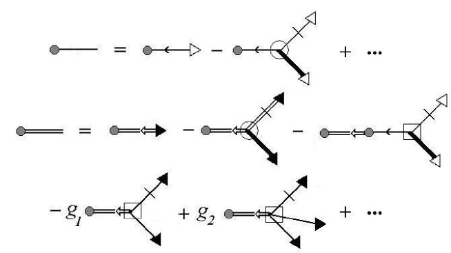
Figure 1: The diagrammatic representation for Eq. (11).

The solutions (11) allow for the diagram representation (see Fig. 1), where the external line (a tail) stands for the field ${n}$, the double external line denotes the field ${w}$, and the bold line represents the magnetic flux $\mathbf{v}$. The triangles stay for the random force $f_{n}$, and the filled triangles represent $f_{w}$. The retarded Green functions $\overleftarrow{\Delta}_{n}$ are marked by the lines with an arrow which corresponds to the arguments $(\mathbf{r^{\prime}},t^{\prime})$ and $(\mathbf{r}^{\prime\prime},t^{\prime\prime})$ (the direction of arrows marks the time ordering of arguments in the lines). Similarly, the double lines with an arrow correspond to the retarded Green functions $\overleftarrow{\Delta}_{w}$. Slashes correspond to the differential operator $\nabla$. Circles surrounding vertices representing the antisymmetric interaction $\mathbf{v}\times\nabla$, squares present the vertices proportional to the poloidal gradient $\partial_{y}.$

All correlation functions of fluctuating fields and functions expressing the system response for the external perturbations could be found by the multiplication of trees (11) displayed on Fig. 1 followed by the averaging over all possible configurations of random forces $f_{n}(\,\mathbf{r},t\,)$ and $f_{w}(\,\mathbf{r},t\,)$. In diagrams, this procedure corresponds to all possible contractions of lines ended with the identical triangles. Thereat, the diagrams having an odd number of external triangles (correspondent to the random forces) give zero contributions in average. As a result of these contractions, the following new elements (lines) appear in the diagrams of perturbation theory:

$$\Delta_{nn}(\mathbf{r}-\mathbf{r^{\prime}},t^{\prime}-t)=\int d\mathbf{r}_{1}dt_{1}\int d\mathbf{r}_{2}dt_{2}{\ }\overrightarrow{\Delta}_{n}(\mathbf{r}-\mathbf{r}_{1},t_{1}-t){D}_{nn}(\mathbf{r}_{1}-\mathbf{r}_{2},t_{1}-t_{2})\overleftarrow{\Delta}_{n}(\mathbf{r}_{2}-\mathbf{r^{\prime}},t_{2}-t^{\prime}),$$

$$\Delta_{ww}(\mathbf{r}-\mathbf{r^{\prime}},t^{\prime}-t)=\int d\mathbf{r}_{1}dt_{1}\int d\mathbf{r}_{2}dt_{2}{\ }\overrightarrow{\Delta}_{w}(\mathbf{r}-\mathbf{r}_{1},t_{1}-t){D}_{ww}(\mathbf{r}_{1}-\mathbf{r}_{2},t_{1}-t_{2})\overleftarrow{\Delta}_{w}(\mathbf{r}_{2}-\mathbf{r^{\prime}},t_{2}-t^{\prime})$$

$$+g^{2}_{1}\partial^{2}_{y}\Delta_{nn}(\mathbf{r}-\mathbf{r^{\prime}},t^{\prime}-t),$$

$$\Delta_{wn}(\mathbf{r}-\mathbf{r^{\prime}},t^{\prime}-t)=g_{1}\int d\mathbf{r}_{1}dt_{1}{\ }\overrightarrow{\Delta}_{n}(\mathbf{r}-\mathbf{r}_{1},t_{1}-t)\partial_{y}\Delta_{ww}(\mathbf{r}_{1}-\mathbf{r^{\prime}},t_{1}-t^{\prime}),$$

$$\overleftarrow{\Delta}_{wn}(\mathbf{r}-\mathbf{r^{\prime}},t^{\prime}-t)=g_{1}\int d\mathbf{r}_{1}dt_{1}{\ }\overleftarrow{\Delta}_{n}(\mathbf{r}-\mathbf{r}_{1},t_{1}-t)\partial_{y}\overleftarrow{\Delta}_{w}(\mathbf{r}_{1}-\mathbf{r^{\prime}},t_{1}-t^{\prime}),$$ (12)

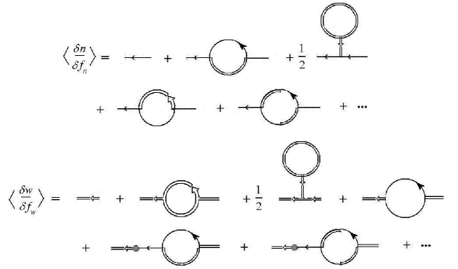
Figure 2: First diagrams for the simplest response functions $\left\langle\delta{n}/\delta f_{n}\right\rangle$ and $\left\langle\delta{w}/\delta f_{w}\right\rangle$.

which are the free propagators of particle density and vorticity fluctuations, the mixed correlator, and the retarded mixed Green’s function. In diagrams, we present the free propagators (12) by the correspondent lines without an arrow, and the retarded mixed Green’s functions by the composite directed lines (see Fig. 2).

The cross-field drift function $\mathbf{v}(\,\mathbf{r},t\,)$ is not involved into the linear homogeneous problem (10) and, therefore, it does not appear in the free propagators (12), however, it is presented in the nonlinear part of dynamical equations and therefore appears in the diagrams of perturbation theory. Due to the simple relation $\mathbf{w}\,=\,\nabla\,\times\mathbf{v}$, the propagators containing the field $\mathbf{v}$ are the same as those with $\mathbf{w}$: $\Delta_{\mathbf{vv}}$, $\Delta_{n\mathbf{v}}$, and $\overleftarrow{\Delta}_{n\mathbf{v}}$. The bold lines representing $\mathbf{v}$ in Fig. 1 can be replaced in the diagrams of perturbation theory with the double lines (which correspond to the field $\mathbf{w}$) with the additional factor (in the momentum representation) $-i\,\varepsilon_{zms}\,k_{m}/k^{2}$, where $m,s\,\equiv\,x,y$ and $\varepsilon_{zxy}$ is the antisymmetric pseudo-tensor, for each $\mathbf{v}$.

In this framework, the exact correlation functions of fields and the response functions can be found from the Dyson equations,

$$\left\langle\,\frac{\,\delta n\,}{\delta f_{n}}\,\right\rangle^{-1}\,=\,\overleftarrow{\Delta}_{n}^{-1}\,-\,\Sigma_{n},\quad\left\langle\,\frac{\,\delta{w}\,}{\delta f_{w}}\,\right\rangle^{-1}\,=\,\overleftarrow{\Delta}_{w}^{-1}\,-\,\Sigma_{w},$$ (13)

where $\Sigma_{n}$ and $\Sigma_{w}$ are the infinite diagram series, in which the first diagrams are shown in Fig. 2. The diagram technique introduced in the present section is suitable for the system preserving the continuous symmetry of (1), apart from the sheath.

4 Functional integral formulation of the stochastic problem. Dimensional analysis, UV divergencies in diagrams and renormalization

In the present section, we study the properties of diagram series resulting from the iterations of the stochastic dynamical equations with the consequent averaging with respect to all possible configurations of random forces. The diagrams for some correlation functions diverge in small scales. The use of conventional arguments borrowed from the quantum field renormalization group [23] helps to prove the consequent subtraction of the logarithmic divergent terms in all orders of perturbation theory out from the diagrams.

The set of diagrams arisen in the perturbation theory by the iterations of (2) is equivalent to the standard Feynman diagrams of some quantum field theory with the doubled set of stochastic fields: the fluctuations ${n}$ and ${w}$, the flux function $\mathbf{v},$ the auxiliary fields $n^{\prime}$, $w^{\prime}$ functionally conjugated to the Gaussian distributed random forces $f_{n}$ and $f_{w}$ in (2), and the Lagrange multiplier $\mathbf{v}^{\prime}$ for the binding relation $\mathbf{w}\,=\,\nabla\,\times\mathbf{v}$. The coincidence of diagrams is a particular consequence of the general equivalence between the $t$-local stochastic dynamical problems (in which the interactions contain no time derivatives) and the relevant quantum field theories [24] with the action functional $\mathcal{S}$ found in accordance to the MSR formalism [12]. Statistical averages with respect to all admissible configurations of random forces in a stochastic dynamical problem can be identified with the functional averages with the weight $\exp\mathcal{S}.$ In particular, for the stochastic problem (2), the generating functional of the Green functions, $\mathcal{G}(A_{\Phi}),$ with the arbitrary source fields $A_{\Phi}(\mathbf{r},t)$ where $\Phi\equiv\{{n},n^{\prime},{w},w^{\prime},\mathbf{v},\mathbf{v^{\prime}}\}$ can be represented by the functional integral

$$\mathcal{G}(A_{\Phi})=\int\mathcal{D}\Phi{\ }\exp\left[\mathcal{S}(\Phi)+\int d\mathbf{r}\,dt{\ }A_{\Phi}(\mathbf{r},t)\Phi(\mathbf{r},t)\right],$$ (14)

in which

$$\mathcal{S}(\Phi)=\frac{1}{2}\int d\mathbf{r}\,d\mathbf{r^{\prime}}\,dt\,dt^{\prime}{\ }\left[n^{\prime}(\mathbf{r},t){D}_{nn}(\mathbf{r}-\mathbf{r^{\prime}},t-t^{\prime})n^{\prime}(\mathbf{r^{\prime}},t^{\prime})+w^{\prime}(\mathbf{r},t){D}_{ww}(\mathbf{r}-\mathbf{r^{\prime}},t-t^{\prime})w^{\prime}(\mathbf{r^{\prime}},t^{\prime})\right]$$ (15)

$$-\,\int\,d\mathbf{r}\,dt{\ }n^{\prime}(\mathbf{r},t)\,\left[\,\partial_{t}{n}(\mathbf{r},t)\,+\,\mathbf{v}(\mathbf{r},t)\,\times\nabla{n}(\mathbf{r},t)\,-\,\nu\Delta_{\bot}{n}(\mathbf{r},t)\,\right]$$

$$-\int d\mathbf{r}\,dt{\ }w^{\prime}(\mathbf{r},t)\left[\partial_{t}{w}(\mathbf{r},t)+\mathbf{v}(\mathbf{r},t)\times\nabla{w}(\mathbf{r},t)+\sum_{k\geq 1}\frac{(-1)^{k}g_{k}}{k}\,\partial_{y}{n}^{k}(\mathbf{r},t)-u_{0}\nu\Delta_{\bot}{w}(\mathbf{r},t)\right]$$

$$+\,\int\,d\mathbf{r}\,dt{\ }\mathbf{v^{\prime}}(\mathbf{r},t)\left[\,{w}(\mathbf{r},t)\,-\,\nabla\,\times\mathbf{v}(\mathbf{r},t)\,\right].$$

The source functions $A_{n^{\prime}}(\,\mathbf{r},t\,)$ and $A_{w^{\prime}}(\,\mathbf{r},t\,)$ in (14) are interpreted as the not random external forces, so that the Green functions $\left\langle\,{w}(\mathbf{r},t)\,w^{\prime}(\mathbf{r^{\prime}},t^{\prime})\,\right\rangle,$ $\left\langle\,{n}(\mathbf{r},t)\,n^{\prime}(\mathbf{r^{\prime}},t^{\prime})\,\right\rangle,$ and $\left\langle\,{n}(\mathbf{r},t)\,w^{\prime}(\mathbf{r^{\prime}},t^{\prime})\,\right\rangle,$ for $t^{\prime}\,<\,t$, coincide with the response functions $\left\langle\,\delta{w}\left/\delta f_{w}\right.\,\right\rangle$, $\left\langle\,\delta{n}\left/\delta f_{n}\right.\,\right\rangle$, and $\left\langle\,\delta{n}\left/\delta f_{w}\right.\,\right\rangle$ respectively. All possible boundary conditions and the damping asymptotic conditions for the fluctuation fields ${n}$ and ${w}$ at $t\,\to-\infty$ are included into the functional integration domain in (14).

The functional integral formulation (14) of the stochastic dynamical problem (2) allows for the use of various techniques developed in the quantum field theory to study the long-time large-scale asymptotic behavior of the quantum and stochastic systems. The integral (14) has the standard Feynman diagram representation which is equivalent to the iterative solution of (2) with an exception of the self-contracted lines $\mathrm{Tr}\left(\overleftarrow{\Delta}_{\Phi\Phi^{\prime}}\right)=\mathrm{Tr}\left(\overleftarrow{\Delta}_{\Phi^{\prime}\Phi}\right)=0,$ which are proportional to $\propto\theta(t-t^{\prime})$ in time-representation and therefore discontinuous at $t=t^{\prime}$. Stipulating that $\theta(0)=0$, one can exclude all redundant graphs from the perturbation theory of (14). Lines and vertices in the graphs of perturbation theory are defined by the conventional Feynman rules and correspond to the free propagators (equivalent to (12)) readily calculated from the free (quadratic) part of functional (15) and the nonlinear interactions of fields respectively. In the actual calculations, it is convenient to use the propagators (12) in their momentum-frequency representation,

$$\overleftarrow{\Delta}_{nn^{\prime}}(k,\omega)=(-i\omega+\nu k^{2})^{-1},\quad\overleftarrow{\Delta}_{ww^{\prime}}(k,\omega)=(-i\omega+u_{0}\nu k^{2})^{-1},\quad\Delta_{w\mathbf{v^{\prime}}}(k)=-{\varepsilon_{zms}k_{s}}/{k^{2}},$$

$$\Delta_{nn}(k,\omega)=\overrightarrow{\Delta}_{nn^{\prime}}D_{nn}(k,\omega)\overleftarrow{\Delta}_{n^{\prime}n},\quad\Delta_{ww}(k,\omega)=g_{1}^{2}k^{2}_{y}\Delta_{nn}(k,\omega)+\overrightarrow{\Delta}_{ww^{\prime}}D_{ww}(k,\omega)\overleftarrow{\Delta}_{w^{\prime}w},$$

$$\Delta_{nw}(k,\omega)=ig_{1}\overleftarrow{\Delta}_{nn^{\prime}}(k,\omega)k_{y}{\ }\Delta_{ww}(k,\omega),\quad\overleftarrow{\Delta}_{nw^{\prime}}(k,\omega)=ig_{1}\overleftarrow{\Delta}_{nn^{\prime}}(k,\omega)k_{y}{\ }\overleftarrow{\Delta}_{ww^{\prime}}(k,\omega),$$

$$\overleftarrow{\Delta}_{nn^{\prime}}(k,\omega)=\overrightarrow{\Delta}^{*}_{nn^{\prime}}(k,\omega),\quad\overleftarrow{\Delta}_{ww^{\prime}}(k,\omega)=\overrightarrow{\Delta}^{*}_{ww^{\prime}}(k,\omega),\quad\overleftarrow{\Delta}_{nw^{\prime}}(k,\omega)=\overrightarrow{\Delta}^{*}_{w^{\prime}n}(k,\omega).$$

Propagators including the field $\mathbf{v}$ coincide with those of the field ${w}$ up to the multiplicative factor $-i\,\varepsilon_{zms}\,k_{m}/k^{2}$ for each field $\mathbf{v}.$ Propagators of auxiliary fields $\Delta_{\Phi^{\prime}\Phi^{\prime}}(k,\omega)=0$.

The action functional (15) is invariant with respect to the generalized Galilean transformations of fields in the poloidal direction,

$${v}_{y}(\,\mathbf{r},t\,)\,\to\,{v}_{y}\left(\,\mathbf{r},t\,\right)\,-\,\mathbf{a}(\,t\,),\quad{n}(x,y,t)\,\to\,{n}\left(\,x,y\,-\,\mathbf{b}(\,t\,),t\,\right)$$ (16)

with the parameter of transformations $\mathbf{a}(\,t\,)$ (the integrable function decaying at $t\,\to-\infty$) and $\mathbf{b}(\,t\,)\,=\,\int_{-\infty}^{t}\,\mathbf{a}(\,t^{\prime}\,)\,dt^{\prime}$. Furthermore, any quantity $Q$ in (15) can be characterized with respect to the independent scale transformations, in space and time, by its momentum dimension $d^{k}_{Q}$ and the frequency dimension $d^{\omega}_{Q}$. In the ”logarithmic” theory (which is free of interactions that is analogous to the linearized problem (10)), these scale transformations are coupled due to the relation $\partial_{t}\sim\nabla^{2}$ in the dynamical equations.

This allows for the introduction of the relevant total canonical dimension $d_{Q}=d^{k}_{Q}+2d^{\omega}_{Q}$ and the analysis of UV divergencies arisen in the diagrams of perturbation theory based on the conventional dimension counting arguments [23, 25]. In dynamical models, $d_{Q}$ plays the same role as the ordinary (momentum) dimension in the critical static problems. Let us note that the poloidal gradient term $\propto\partial_{y}$ in (10) is responsible for the stationary contributions into the Green’s function as $t>0$, so that the above definition of $d_{Q}$ remains unambiguous. Stipulating the natural normalization conventions, $d^{k}_{k}=-d^{k}_{\mathbf{r}}=1,$ ${\ }d^{\omega}_{k}=d^{\omega}_{\mathbf{r}}=0,$ ${\ }d^{k}_{\omega}=d^{k}_{t}=0,$ ${\ }d^{\omega}_{\omega}=-d^{\omega}_{t}=1$, one can find all relevant canonical dimensions from the simultaneous momentum and frequency scaling invariance of all terms in (15) (see Tab. 1).

Integrals correspondent to the diagrams of perturbation theory representing the 1-irreducible Green’s functions $G$ diverge at the large momenta (small scales) if the correspondent UV-divergence index $\delta_{G}$ is a nonnegative integer in the logarithmic theory,

$$\delta_{G}=d+2-\left(N_{\Phi}d_{\Phi}+N_{\Phi^{\prime}}d_{\Phi^{\prime}}\right)\geq 0,$$ (17)

where $d$ is the dimension of space, $d_{\Phi,\Phi^{\prime}}$ are the total canonical dimensions of fields $\Phi$ and $\Phi^{\prime}$, and $N_{\Phi,\Phi^{\prime}}$ are the numbers of relevant functional arguments in $G$. As a consequence of the casualty principle, in the dynamical models of MSR-type, all 1-irreducible Green’s functions without the auxiliary fields $\Phi^{\prime}$ vanish being proportional to $\theta(0)$ and therefore do not require counterterms [17]. Furthermore, the dimensional parameters and external momenta occurring as the overall factors in graphs also reduce their degrees of divergence (17).

In spite of the following 1-irreducible Green functions could be superficially divergent at large momenta: $\langle n^{\prime}{n}\mathbf{v}\rangle$, $\langle n^{\prime}\mathbf{v}\rangle$, $\langle n^{\prime}\mathbf{v}\mathbf{v}\rangle$, $\langle n^{\prime}{n}\ldots{n}\rangle$ (with an arbitrary number of fields ${n}$ ), the only Galilean invariant Green’s function admissible in the theory (15) which actually diverges at large momenta is $\langle n^{\prime}{n}\rangle$. The inclusion of the relevant counterterm subtracting their superficially divergent contribution is reproduced by the multiplicative renormalization of the Prandtl number

$$u_{0}=uZ_{u}$$

where $u_{0}$ and $u$ are the bare and renormalized values of Prandtl’s number. In principle, the relevant renormalization constant $Z_{u}$ can be calculated implicitly from the graphs of perturbation theory up to a finite part of the relevant counterterm.

However, the standard approach of the critical phenomena theory is useless for the determining of the large scale asymptotes in the problem in question, since the severe instability frustrates the critical behavior in the system preventing its approaching to the formal asymptote predicted by the conventional renormalization group method. As a consequence, the critical dimensions of fields and parameters which can be computed from the renormalization procedure would have just a formal meaning.

5 Large scale instability of iterative solutions

The iterative solutions for the stochastic problem (2) constructed in Sec. 3 would be asymptotically stable in the large scales provided all small perturbations of both density and vorticity damp out with time. In particular, the exact response functions found from the Dyson equations (13) should have poles located in the lower half-plane of the frequency space.

The stability of free response function $\left.\left\langle\,\delta n\right/\delta f_{n}\,\right\rangle\,=\,(-i\omega\,+\,\nu\,k^{2})^{-1}$ which effectively corresponds to the linearized problem (10) is ensured in the large scales by the correct sign of the dissipation term $\nu k^{2}\,>\,0$. In a ”proper” perturbation theory, apart from a crossover region, the stability of exact response functions is also secured by the dissipation term which dominates over the dispersion relation in the large scales,

$$\omega(\,k\,)\,=\,-i\,\nu k^{2}\,+\,i\,\Sigma_{nn}(\,k,\omega\,)$$ (18)

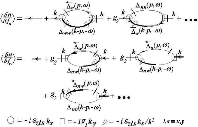
Figure 3: The simplest 1-irreducible diagrams contributing into the self-energy corrections $\Sigma_{nn}$ and $\Sigma_{nw}$ for the response functions $\left\langle\delta{n}/\delta f_{n}\right\rangle$ and $\left\langle\delta{n}/\delta f_{w}\right\rangle$. The field indices denote the type of propagators and simultaneously the type of vertexes. The slashes mark the positions of derivatives $\nabla$, and the skewed triangles denotes the inverse operator $\mathrm{curl}^{-1}$.

where the self-energy operator $\Sigma_{nn}(\,k,\omega\,)$ is the infinite series of all relevant $1-$irreducible diagrams of perturbation theory. However, in the perturbation theory discussed in Sec. 3, the leading contribution into the self-energy operator is $\Sigma_{nn}\,\simeq\,O(\,k_{y}\,)$ that could lift up the pole of the response function into the upper half-plane of the complex $\omega-$plane rising the instability in the system as $k\,\to\,0$. Such an anomalously strong contribution comes from the diagrams which simultaneously include both the antisymmetric interaction vertex $\simeq i\,\mathrm{e}_{z}\cdot\,\varepsilon_{ijz}\,\mathrm{v}_{i}k_{j}$ together with the poloidal gradient $\simeq i\,g_{k}\,k_{y}$ and the free propagator of particle density $\Delta_{nn}(\,k,\omega\,)$. Such diagrams appear in all orders of perturbation theory for the response functions $\left.\left\langle\,\delta{n}\right/\delta f_{n}\,\right\rangle$ and $\left.\left\langle\,\delta{n}\right/\delta f_{w}\,\right\rangle$ indicating that the instability could arise due to the random fluctuations of both density and vorticity. The first order 1-irreducible diagrams for them are displayed in Fig. 3. The small parameters $g_{n}$ with $n\,>\,2$ appear in the forthcoming orders of perturbation theory. In particular, the last diagrams in both series shown in Fig. 3 generate the ”anomalous” contributions in the large scales.

To be certain, let us consider the second diagram in the series for $\left.\left\langle\,\delta{n}\right/\delta f_{n}\,\right\rangle$ which corresponds to the following analytical expression:

$$\left.\Sigma_{nn}\right|_{\mathrm{1-loop}}\,\simeq\,g_{2}k_{y}\,\int\frac{d\mathbf{p}}{(2\pi)^{2}}\,\int\frac{d\omega}{2\pi}\,\int\frac{d\omega^{\prime}}{2\pi}\,\,\frac{k_{x}p_{x}+k_{y}p_{y}-p_{x}^{2}-p^{2}_{y}}{(\mathbf{k-p})^{2}}\,\,\Delta_{nn}(\mathbf{p},\omega^{\prime})\,\,\overleftarrow{\Delta}_{w}(\mathbf{k}-\mathbf{p},\omega-\omega^{\prime}).$$ (19)

Being interested in the $O(\,k_{y}\,)$-contribution into (19), one can neglect the $k-$dependence in the integrand. The analytical properties of this contribution depends very much upon the certain assumption on the covariances of random forces since it changes the free propagator $\Delta_{nn}$. For instance, under the white noise assumption (3) $\Delta_{nn}\,\simeq\,(\,\omega^{2}\,+\,\nu^{2}p^{4}\,)^{-1},$ the integral in (19) diverges at the small scales (large momenta) for $\varepsilon\,<\,1$ and diverges at the large scales (small momenta) for $\varepsilon\,>\,1$. Introducing the relevant cut-off parameters, one obtains the anomalous contribution

$$\left.\Sigma_{nn}\right|_{\mathrm{1-loop}}\,\simeq\,-\,\,k_{y}\,{\frac{\nu\,g_{2}\left({\Lambda}^{2-2\,\varepsilon}-{m}^{2-2\,\varepsilon}\right)}{8\pi\,\left(-1+\varepsilon\right)\left(u+1\right)}},$$ (20)

in which $u$ is the renormalized value of Prandtl’s number. In the preceding section, we have shown that the logarithmic divergencies risen in diagrams for the response function $\left.\left\langle\,\delta n\right/\delta f_{n}\,\right\rangle$ in the small scales (large momenta) can be eliminated from the perturbation theory by the appropriate renormalization. The singularity in (20) arisen at the small momenta $m\to\,0$ for $\varepsilon\,>\,1$ would compensate the smallness of $g_{2},$ so that any density fluctuation with $k_{y}\,>\,0$ appears to be unstable.

Accounting for the finite reciprocal correlation time $\tau_{c}\,>\,0$ between the vorticity and density random sources in (2) introduces the new dimensional parameter $\lambda>0$ into the particle density propagator, $\Delta_{nn}\,\simeq\,\left(\,\omega^{2}\,+\,\nu^{2}p^{4}\,\left(1\,+\,\lambda\,p^{-2\gamma}\,\right)\,\right)^{-1}.$ Then, the integral (19) can be computed by its analytic continuation for any momenta excepting for the isolated points, $-1+\varepsilon=\gamma\,\mathrm{mod}\,1,$

$$\Sigma_{nn}\,=\,\nu\,A\,(\,\varepsilon,\gamma\,)\,\,k_{y},\quad\left.A\,(\,\varepsilon,\gamma\,)\right|_{\mathrm{1-loop}}\,\simeq\,k_{y}\,\,\frac{1}{8}\,\left({\frac{u}{\lambda}}\right)^{(-1+\varepsilon)/\gamma}\frac{\nu}{{u}}\,\frac{g_{{2}}}{{\gamma}}\csc\left({\frac{\pi\,\left(-1+\varepsilon\right)}{\gamma}}\right).$$ (21)

The dispersion relation (18) determines the region of asymptotic stability in the phase space of cross-field transport system. Namely, a density fluctuation arisen in the SOL with some random momenta $(k_{x},\,k_{y})$ would be asymptotically stable with respect to the large scales $k\,\to\,0$ if

$$\frac{\,\,k_{y}\,\,}{\,k_{x}^{2}\,+\,k_{y}^{2}\,}\,<\,\frac{1}{A\,(\,\varepsilon,\,\gamma\,)}$$ (22)

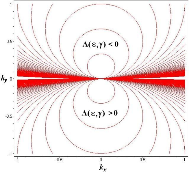
Figure 4: . The admissibility condition (22) defines the set of elliptic curves which bound the unstable segments in the phase space. Density fluctuations with $k_{y}\,\to\,0,$ (i.e. extended in the poloidal direction) appear to be stable in the large scales for any $|\,k_{x}\,|\,>\,0$. Those fluctuations characterized by $|\,k_{y}\,|\,>\,0$ would also be stable in the large scales provided $\mathrm{sign}\,\left(\,k_{y}\,\right)\,=\,-\,\mathrm{sign}\,\left(\,A(\varepsilon,\gamma)\,\right)$ for the given values $\varepsilon$ and $\gamma$.

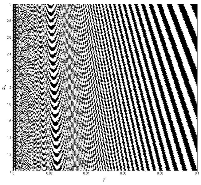
Figure 5: . The signature of 1-loop order contribution (21) into $A(\varepsilon,\gamma)$ (black is for $+1,$ white is for $-1$) at different values of $\gamma$ and $d=6-2\varepsilon-2\gamma$, the space dimension related to the actual value of regularization parameter $\varepsilon$ under the statistical assumption (8).

and be unstable otherwise. In the first order of perturbation theory, the amplitude factor $A(\varepsilon,\gamma)$ is given by (21). For different values $A\,(\,\varepsilon,\,\gamma\,),$ the stability condition (22) determines the set of circles (see Fig. 4) osculating at the origin which bound the unstable segments of phase space. One can see that the density fluctuations with $k_{y}\,\to\,0$ (i.e. extended in the poloidal direction) are asymptotically stable for any $|\,k_{x}\,|\,>0$. Density fluctuations characterized by $|\,k_{y}\,|\,>0$ would be asymptotically stable in a certain stochastic model provided $\mathrm{sign}\,\left(\,k_{y}\,\right)\,=\,-\,\,\mathrm{sign}\,\left(A(\,\varepsilon,\gamma\,)\right),$ for the given values of $\varepsilon$ and $\gamma$. The signature of the 1-loop order contribution (21) into $A(\,\varepsilon,\gamma\,)$ is displayed on the diagram in Fig. 5 (black is for $+1,$ white is for $-1$) at different values of $\gamma$ and $d=6-2\varepsilon-2\gamma$, the space dimension related to the actual value of regularization parameter $\varepsilon$ under the statistical assumption (8).

It is important to note that the stability condition (22) can be formulated as an upper bound for the order parameter $\xi=\left.\,k_{y}\,\right/\,k^{2}$: $\,\;\xi\,<\,\xi_{c}$ where $\xi_{c}\,=\,A\,(\,\varepsilon,\,\gamma\,)^{-1}$. For the uncorrelated statistics of random forces, in the stochastic dynamical problem, $A(\,\varepsilon,\gamma\,)$ (20) diverges as $k\to 0$ and therefore $\xi_{c}\,\to\,0.$

6 Turbulence stabilization by the poloidal electric drift

To promote the stochastic cross-field turbulent transport system (2) from the instability to a stable regime, it seems natural to frustrate the symmetry which breaks the Galilean invariancy in (2). This can be achieved by generating a constant uniform drift in the poloidal direction $\mathrm{v}_{y}\,\to\,\mathrm{v}_{y}\,-\,V$ (by biasing the limiter surface, $\phi(x)\,\to\,\phi(x)+\,xV$) that would eradicate those configurations with the trivial poloidal component of electric drift $\mathrm{v}_{y}\,=\,0.$ In general, the relevant dispersion equation $\omega\,(\,k,V\,)\,=\,0$ could have many solutions $V_{k}$ for $k\,\ll\,1.$ Herewith, the turbulence stabilization is achieved for the drifts $V$ from the intervals $V_{k-1}\,<\,V\,<\,V_{k}$ for which $\mathrm{Im}(\omega)\,<\,0.$

To be certain, let us consider the dispersion equation correspondent to the simplest response function $\left.\left\langle\,\delta n\right/\delta f_{n}\,\right\rangle$, in the 1-loop order. The leading contribution into the dispersion equation is given in the large scale region by the diagram (19). Under the white noise assumption (3), the free propagator accounting for the uniform electric drift $V$ is $\Delta_{nn}\,\simeq\,\left(\,{\omega}^{2}\,+\,{\nu}^{2}{k}^{4}\,+\,{V}^{2}{k_{{y}}}^{2}\,\right)^{-1}$. Then, for $|\,k_{y}\,|\,<\,1$, the dispersion relation reads as following,

$$\omega(\,k,\,V\,)\,\simeq\,-i\,\nu\,{k}^{2}\,+\,i\,k_{{y}}\,\,\frac{g_{{1}}g_{{2}}}{u+1}\left(\,{\frac{\nu\,\left({m}^{2-2\,\varepsilon}\right)}{8\pi\,\left(-1+\varepsilon\right)}}-\,\sqrt{\pi}\,{\frac{\,{V}^{2}\left(u+2\right)\,\Gamma\left(1/2+\varepsilon\right)\,\log m}{8\nu\,\left(1+u\right)\,\Gamma\left(2+\varepsilon\right)}}\right).$$ (23)

The latter relation shows that for any finite $m\,>\,0$ there exists finite $V_{c}\,<\,\infty$ such that for any $V\,>\,V_{c}$ one obtains $\mathrm{Im}(\omega)\,<\,0$ in (23), however, $V_{c}\,\to\,\infty$ as $m\,\to\,0.$

In contrast to it, in the case of correlated statistics (4 - 5, 8), the dispersion relation is not singular for $k\,\to\,0$ excepting some particular values of $\varepsilon$ and $\gamma$, and the correspondent stabilizing electric drift, in the 1-loop order, equals to

$$V_{c}\,=\,\pi\,\nu{u}^{3}\,\,\frac{\,\left(u\lambda\right)^{1/2{\gamma}}\left(1+u\right)^{1\,+\,\,(2\varepsilon+1)/2\gamma}\,\,\left(\,\left(\,1+u\,\right)^{1+\,{\varepsilon}/{\gamma}}-1\,\right)}{\,\left(1+u\right)^{2\,+\,\,(2\varepsilon+1)/2\gamma}+u\left(2\,\varepsilon+1\right)-2\,\gamma\,\left(1+2\,u\right)\,\,}\,\,\,\frac{\,\sin\,\left.{\pi\,(\,2\varepsilon\,+\,1\,)}\right/{2\gamma}}{\,\sin\,{\pi\,\varepsilon}\,/{\gamma}}.$$ (24)

In the range $0\,<\,\gamma\,<\,1/2$, $\,\,u\,>\,0$, this expression is singular at the points $\varepsilon\,/\gamma\,\in\,\mathbb{Z}$.

7 Qualitative discrete time model of anomalous transport in the SOL

Large scale instability developed in the cross-field model (2) is related to the appearance and unbounded growth of fluctuations of particle density close to the wall. In accordance to the fluctuation-dissipation theorem, the fluctuations arisen in the stochastic dynamical system are related to its dissipative properties. In particular, the matrix of the exact response functions $\mathbb{R}(\,\mathbf{k},\omega\,)$ expressing the perturbations of fields $n$ and $w$ risen due to the random sources $f_{n}$ and $f_{w}$ determines the matrix of exact dynamical Green’s functions $\mathbb{G}(\,\mathbf{k},\omega\,),$

$$\mathbb{R}\,(\,\mathbf{k},\,\omega\,)\,-\,\mathbb{R}^{\dagger}\,(\,\mathbf{-k},\,-\omega\,)\,=\,i\,\omega\,\mathbb{G}\,(\,\mathbf{k},\,\omega\,)$$ (25)

where $\mathbb{R}^{\dagger}$ is the transposed $\mathbb{R}.$ In the large scale limit $k\to 0$, we take into account for the leading contributions into the self-energy operators in the elements of $\mathbb{R}$,

$${R}_{nn}\,\simeq\,\left(-i\omega\,-\nu\,A_{1}\,k_{{y}}\,+\nu\,{k}^{2}\right)^{-1},\quad R_{nw}\,\simeq\,\left(-i\omega\,-\,\nu\,u\,A_{2}\,k_{y}\,+\nu\,u\,{k}^{2}\right)^{-1},$$ (26)

$${R}_{wn}\,\simeq\,\left(-i\omega\,+\nu\,{k}^{2}\right)^{-1},\quad R_{ww}=\,\left(-i\omega\,+\nu u\,{k}^{2}\right)^{-1},$$

in which $A_{1,2}$ are the amplitudes of the anomalous contributions competing with the dissipation $\propto O(k^{2})$ in the large scales. Fluctuations of particle density arisen in the model (2) grow up unboundedly provided either $A_{1}\,k_{y}\,>\,k^{2}$ or $A_{2}\,k_{y}\,>\,k^{2}$ for the given values of $\varepsilon$ and $\gamma.$ The correspondent advanced Green’s functions appear to be analytic in the lower half-plane of the frequency space,

$$\nu\cdot G^{a}_{nn}\,(\,\mathbf{k},t\,)=\,\frac{A_{1}\,k_{y}\,\,\theta(-t)}{\,k^{4}\,-\,A_{1}^{2}\,k_{y}^{2}},\quad\nu\,u\cdot G^{a}_{nw}\,(\,\mathbf{k},\,t\,)=\,-\frac{\theta(-t)}{\left(A_{2}\,k_{y}\,-\,k^{2}\right)}-\frac{\theta(-t)}{k^{2}},$$ (27)

being trivial for $t\,>\,0.$

For instance, let us consider the advanced Green’s function $G^{a}_{nn}$ which relates the density of particles ${\delta\!n}(\,\mathbf{r},\,t\,)$ in the fluctuations characterized with $A_{1}\,k_{y}\,>\,k^{2}$ and arisen at the point $\mathbf{r}\in\Omega$ inside the divertor at time $t$ with the particle density ${\delta\!n}(\,\mathbf{r^{\prime}},\,t^{\prime}\,)$ of those achieved the divertor wall at some subsequent moment of time $t^{\prime}\,>\,t$ at the point $\mathbf{r^{\prime}}\in\partial\Omega$:

$$\left.{\delta\!n}(\,\mathbf{r^{\prime}},\,t^{\prime}\,)\right|_{\partial\Omega}\,=\int_{\,t\,<\,t^{\prime}}\,dt\,\,\int_{\Omega}\,d\mathbf{r}\,\,{\delta\!n}(\,\mathbf{r},\,t\,)\,G^{a}_{nn}(\,\mathbf{r^{\prime}-r}\,)$$ (28)

where

$$G^{a}_{nn}\left(\mathbf{r^{\prime}}-\mathbf{r}\right)=\frac{1}{2\nu\,A_{1}}\,\left[\sin\frac{A_{1}(y^{\prime}-y)}{2}\,{J}_{0}\left(\frac{A_{1}|r^{\prime}-r|}{2}\right)+\cos\frac{A_{1}(y^{\prime}-y)}{2}\,{H}_{0}\left(\frac{A_{1}|r^{\prime}-r|}{2}\right)\right],$$ (29)

in which $\left|r-r^{\prime}\right|\equiv\sqrt{(x-x^{\prime})^{2}+(y-y^{\prime})^{2}},$ $J_{0}$ and $H_{0}$ are the Bessel and Struve functions respectively. The integral in the r.h.s. of (28) is finite for any $\Omega$ provided $|\,A_{1}\,|\,>\,1,$ but for the compact $\Omega$ as $|\,A_{1}\,|\,<\,1$. To be specific, let us consider the circle $C_{R}$ of radius $R$ as the relevant domain boundary and suppose for a simplicity that the density of particles incorporated into the growing fluctuations inside the domain is independent of time and maintained at the stationary rate $\delta\!n_{0}(\,\mathbf{r})$. Then the $\mathbf{r}-$integral in the r.h.s of (28) can be calculated at least numerically and gives the growth rate $B(R)$ for those density fluctuations,

$${\delta\!n}(\,R,\,\tau\,)\,=\,\tau\,\cdot B(R)\,,$$ (30)

where $\tau$ is the travelling time of the density blob to achieve the divertor wall that can be effectively considered as a random quantity. It is the distribution of such wandering times that determines the anomalous transport statistics described by the flux pdf in our simplified model. The discrete time model we discuss below is similar to the toy model of systems close to a threshold of instability studied in [8] recently. Despite its obvious simplicity (the convection of a high density blob of particles by the turbulent flow of the cross field system is substituted by the discrete time one-dimensional (in the radial direction) random walks characterized with some given distribution function), its exhibits a surprising qualitative similarity to the actual flux driven anomalous transport events reported in [4].

We specify the random radial coordinate of a growing fluctuation by the real number $x\,\in\,[0,\,1].$ Another real number $R\,\in\,[0,\,1]$ is for the coordinate of wall. The fluctuation is supposed to be convected by the turbulent flow and grown as long as $x\,<\,R$ and is destroyed otherwise ($x\,\geq\,R$). We consider $x$ as a random variable distributed with respect to some given probability distribution function $\mathbb{P}\{x<u\}=F(u)$. It is natural to consider the coordinate of wall $R$ as a fixed number, nevertheless, we discuss here a more general case when $R$ is also considered as a random variable distributed over the unit interval with respect to another probability distribution function (pdf) $\mathbb{P}\,\{R\,<\,u\}=Q(u)$. In general, $F$ and $Q$ are two arbitrary left-continuous increasing functions satisfying the normalization conditions $F(\,0\,)\,=\,Q(\,0\,)\,=\,0$, $F(\,\infty\,)\,=\,Q(\,\infty\,)\,=\,1$.

Given a fixed real number $\eta\,\in\,[0,1]$, we define a discrete time random process in the following way. At time $t\,=\,0,$ the variable $x$ is chosen with respect to pdf $F$, and $R$ is chosen with respect to pdf $Q$. If $x\,<\,R$, the process continues and goes to time $t\,=\,1$. Otherwise, provided $x\,\geq\,R,$ the process is eliminated. At time $t\,\geq\,1,$ the following events happen:

i) with probability $\eta$, the random variable $x$ is chosen with pdf $F,$ but the threshold $R$ keeps the value it had at time $t\,-\,1$. Otherwise,

ii) with probability $1\,-\,\eta,$ the random variable $x$ is chosen with pdf $F$, and $R$ is chosen with pdf $Q$.

If $x\,\geq\,R,$ the process ends; if $x\,<\,R,$ the process continues and goes to time $t\,+\,1.$

Eventually, at some time step $\tau,$ when the coordinate of the blob, $x,$ drops ”beyond” $R,$ the process stops, and the integer value $\tau$ resulted from such a random process limits the duration of convectional phase. The new blob then arises within the domain, and the simulation process starts again.

While studying the above model, we are interested in the distribution of durations of convection phases $P_{\eta}(\tau;\,F,Q)$ (denoted as $P(\tau)$ in the what following) provided the probability distributions $F$ and $Q$ are known, and the control parameter $\eta$ is fixed. The motionless wall corresponds to $\eta=0.$ Alternatively, the position of wall is randomly changed at each time step as $\eta=1.$

The proposed model resembles to the coherent-noise models [26]-[27] discussed in connection with a standard sandpile model [20] in self-organized criticality, where the statistics of avalanche sizes and durations take power law forms.

We introduce the generating function of $P(\,\tau\,)$ such that

$$\hat{P}(s)\,=\,\sum_{\tau=0}^{\infty}\,s^{\tau}\,\,P(\,\tau\,),\quad P(\tau)\,=\,\left.\frac{1}{\,\tau!\,}\,\frac{d^{\tau}\,\hat{P}(\,s\,)}{ds^{\tau}}\,\right|_{s=0},$$ (31)

and define the following auxiliary functions

$$K(n)\,=\,\int_{0}^{\infty}\,F(u)^{n}\,dQ(u),\quad\delta\!K(n)\,=\,K(n)\,-\,K(n+1),$$

$$\begin{array}[]{lll}p(l)\,=\,\eta^{l}\,\,K(l+1)\;,&\quad\mathrm{for}{\ }l\geq 1\;,&\quad p(0)=0\;,\\ q(l)\,=\,(1-\eta)^{l}\,\,K(1)^{l-1}\;,&\quad\mathrm{for}{\ }l\geq 1\;,&\quad q(0)=0\;,\\ r(l)\,=\,\eta^{l}\,\left[\eta\,\,\delta\!K\,(l+1)\,+\,(1-\eta)\,K(l+1)\,\,\delta\!K(0)\right]\;,&\quad\mathrm{for}{\ }l\geq 1,&\quad r(0)=0\;,\\ \rho=\eta\,\,\delta\!K(1)+(1-\eta)\,\,K(1)\,\,\delta\!K(0)\;.&&\end{array}$$ (32)

Then we find

$$\hat{P}(s)=\delta\!K(0)+\rho s+\frac{s}{1-\hat{p}(s)\hat{q}(s)}\left[\hat{r}(s)+\rho\hat{p}(s)\hat{q}(s)+\rho\,\,K(1)\hat{q}(s)+K(1)\,\,\hat{q}(s)\hat{r}(s)\right]\;,$$ (33)

where $\hat{p}(s),\hat{q}(s),\hat{r}(s)$ are the generating functions corresponding to $p(l),q(l),r(l),$ respectively.

In the marginal cases $\eta=0$ and $\eta=1$, the probability $P(\tau)$ can be readily calculated,

$$P_{\eta=0}(\tau)\,=\,K(1)^{\tau}\,\,\delta\!K(0),\quad P_{\eta=1}(\tau)=\delta\!K(\tau).$$ (34)

The above equation shows that in the case of $\eta\,=\,0,$ for any choice of the pdf $F$ and $Q$, the probability $P(\tau)$ decays exponentially. In the opposite case $\eta\,=\,1,$ many different types of behavior are possible, depending upon the particular choice of $F$ and $Q$.

To estimate the upper and lower bounds for $P(\tau)$ for any $\eta$, one can use the fact that

$$K(1)^{n}\leq K(n)\leq K(1)\;\;\;\;\mbox{and}\;\;\;\;0\leq\delta\!K(n)\leq K(1)\;,\;\;\;\;\;n\,\in\,\mathbb{N}.$$

Then the upper bound for $K(n)$ is trivial, since $0\leq F(u)\leq 1$ for any $u\in[0,1]$. The upper bound for $K(n)$ exists if the interval of the random variable $u$ is bounded and therefore can be mapped onto $[0,1]$ (as a consequence of Jensen’s inequality, and of the fact that the function $u:\rightarrow u^{n}$ is convex on the interval $]0,1[$ for any integer $n$). The calculation given in [8] allows for the following estimation for the upper bound,

$$P_{\eta}(\tau) \leq \eta^{\tau}\,\,\delta\!K(\tau)+(1-\eta)K(1)\,\,\delta\!K(0)\left[\eta+(1-\eta)\,\,K(1)\right]^{\tau-1}$$

$$+ \eta\,\,K(1)\,\,\left\{\left[\eta+(1-\eta)\,\,K(1)\right]^{\tau-1}-\eta^{\tau-1}\right\}\;,$$

and, for the lower bound,

$$P_{\eta}(\tau) \geq \eta^{\tau}\,\,\delta\!K(\tau)+(1-\eta)\,\,K(1)^{\tau}\,\,\delta\!K(0)$$

$$= \eta^{\tau}P_{\eta=1}(\tau)+(1-\eta)P_{\eta=0}(\tau)\;.$$

We thus see that, for any $0\leq\eta<1$, the decay of distribution $P(\tau)$ is bounded by exponentials. Furthermore, the bounds (7) and (7) turns into exact equalities, in the marginal cases $\eta=0$ and $\eta=1$.

The simpler and explicit expressions can be given for $P(\tau)$ provided the densities are uniform $dF(u)=dQ(u)=du$ for all $u\in[0,1]$. Then the equations (34) give,

$$P_{\eta=0}(\,\tau\,)\,=\,2^{-\,(\tau\,+\,1)},\quad P_{\eta=1}(\,\tau\,)\,=\,\frac{1}{(\tau\,+\,1)(\tau\,+\,2)}.$$ (37)

For the intermediate values of $\eta$, the upper and lower bounds are

$$\frac{\eta^{\tau}}{(\tau\,+\,1)(\tau\,+\,2)}\,+\,(1-\eta)\,2^{-\,(\tau\,+\,1)}\,\leq\,P(\,\tau\,)\leq\frac{1}{2}\,\,\left(\,\frac{1\,+\,\eta}{2}\,\right)^{\tau}.$$ (38)

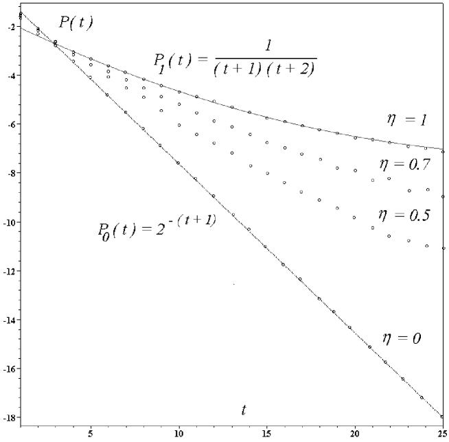
Figure 6: . The distributions of wandering times near the wall in the discrete time model of Sec. 7, in the case of the uniform densities $dF(u)\,=\,dG(u)\,=\,du$ for all $u\in[0,\infty)$ at different values of control parameter $\eta$.

The above results are displayed in Fig. 6.

8 Conclusion

In the present paper, we have considered the stochastic model of turbulent transport in the SOL of tokamak. This problem allows for the concurrent symmetries, and the system exhibits a sever instability with respect to both perturbations either particle density or vorticity. Instability would reveal itself in the appearance of high density blobs of particles hitting into the reactor wall.

The accounting for the dissipation processes introduces the order parameter $\xi=\left|k_{y}\right|\left/\left(k^{2}_{x}+k_{y}^{2}\right)\right.$ and its critical value $\xi_{c}$ such that the particle density fluctuation $\delta\!n(\xi)$ grows unboundedly with time as $\xi\,>\,\xi_{c}$ and damps out otherwise. In the present paper, we compute the value of $\xi_{c},$ in the first order of perturbation theory developed with respect to the small parameter $\left.\rho_{s}\,\right/R\bar{n}$ where $\rho_{s}$ is the Larmor radius, $R$ is the major radius of torus, and $\bar{n}$ is the mean normalized density of particles.

Our results demonstrate convincingly that the possible correlations between density and vorticity fluctuations would drastically change the value $\xi_{c}$ modifying the stability of model. Characterizing the possible reciprocal correlations between the density and vorticity fluctuations by the specific correlation time $\tau_{c}$, we demonstrate that any fluctuation of particle density grows up with time in the large scale limit ($k\to 0$) as $\tau_{c}\to\infty$ (the density and vorticity fluctuations are uncorrelated) and therefore $\xi_{c}=0.$ Alternatively, $\xi_{c}>0$ provided $\tau_{c}<\infty$.

The reciprocal correlations between the fluctuations in the divertor is of vital importance for a possibility to stabilize the turbulent cross field system, in the large scales, by biasing the limiter surface discussed in the literature before [4]. Namely, if $\xi_{c}>0$, there would be a number of intervals $[V_{k-1},V_{k}]$ for the uniform electric poloidal drifts $V$ such that all fluctuations arisen in the system are damped out fast. In particular, in the first order of perturbation theory, there exists one threshold value $V_{c}$ such that the instability in the system is bent down as $V\,>\,V_{c}.$ However, $V_{c}\to\infty$ as $\xi_{c}\to 0.$

To get an insight into the statistics of growing fluctuations of particle density that appear as high-density blobs of particles close to the reactor wall, we note that their growth rates are determined by the advanced Green’s functions analytical in the lower half plain of the frequency space. We replace the rather complicated dynamical process of creation and convection of growing density fluctuations by the turbulent flow with the problem of discrete time random walks concluding at a boundary. Such a substitution can be naturally interpreted as a Monte Carlo simulation procedure for the particle flux. Herewith, the wandering time spectra which determine the pdf of the particle flux in such a toy model are either exponential or bounded by the exponential from above. This observation is in a qualitative agreement with the numerical data reported in [4].

9 Acknowledgment

Authors are grateful to the participants of the Journées de Dynamique Non Linéaire on 2 December 2003, Luminy, Marseille (France) for the valuable discussions. One of the authors (D.V.) deeply thanks the Centre de Physique Theorique (CNRS), Marseille, where the present work had been started.

Table 1: Canonical dimensions of fields and parameters in the action functional (15)

	$\nu$	$u_{0}$	$n$	$w$	$\mathbf{v}$	$\mathbf{v^{\prime}}$	$n^{\prime}$	$w^{\prime}$	$\phi$	$g_{k}$
$d^{k}$	-2	0	0	0	-1	$d$	$d$	$d$	-2	$-1$
$d^{\omega}$	1	0	0	1	1	0	0	2	1	2
$d$	0	0	0	2	1	$d$	$d$	$d+4$	0	3

10 Figures:

References

- [1] D. L. Rudakov et al 2002 Plasma Phys. Control. Fusion 44 2041.
- [2] B. Labombard et al 2000 Nucl. Fusion 40 2041.
- [3] G. Y. Antar, P. Devynck, X. Garbet, S. C. Luckhardt 2001 Phys. Plasmas 8 1612.
- [4] Ph. Ghendrih et al 2003 Nucl. Fusion 43 1013.
- [5] A. V. Nedospasov et al. 1989 Sov. J. Plasma Phys. 15 659.
- [6] X. Garbet et al. 1991 Nucl. Fusion 31 967.
- [7] R. Z. Sagdeev, G. M. Zaslavsky, in Nonlinear Phenomena in Plasma Physics and hydrodynamics. Edited by R. Z. Sagdeev, Mir Publishers, Moscow (1986).
- [8] E. Floriani, D. Volchenkov, R. Lima, Journ. Phys. A: Math. Gen. 36 4771 (2003).
- [9] J. Gunn, Phys. Plasmas 8 1040 (2001).
- [10] P. C. Stangeby, M. C. McCracken, Nucl. Fusion 30 1225 (1990).
- [11] B. Labombard, Phys. Plasmas 9 1300 (2002).
- [12] P. C. Martin, E. D. Siggia, H. A. Rose, Phys. Rev. A8 423 (1973).
- [13] S. K. Ma, Modern Theory of Critical Phenomena, Benjamin Reading (1976).
- [14] B. A. Carreras et al., Phys Plasmas 3 2664 (1996).
- [15] G. Pelletier, J. Plasma Phys. 24 421 (1980), L. Ts. Adzhemyan, A. N. Vassilev, M. Hnatich, Yu. Pismak, Theor. Math Phys. 78 368 (1989) (in Russian).
- [16] V. E. Zaharov, JETP 62 1745 (1972) (in Russian).
- [17] L. Ts. Adzhemyan, N. V. Antonov, A. N. Vasiliev, The Field Theoretic Renormalization Group in Fully Developed Turbulence, Gordon and Breach (1999).
- [18] N. V. Antonov, Anomaluous scaling of a Passive Scalar Advected by the Symmetric Compressible Flow, arXiv: chao-dyn/ 9808011 (1998); chao-dyn/9907018 (1999).
- [19] D. Volchenkov, B. Cessac, Ph. Blanchard, Intern. Jour. of Modern Phys. B 16 (08), 1171 (2002).
- [20] P. Bak, C. Tang, K. Wiesenfeld, Phys. Rev. Lett. 59, 381 (1987).
- [21] Y.-C. Zhang, Phys. Rev. Lett. 63, 470 (1989).
- [22] Bak P. How nature works, Springer-Verlag (1996).
- [23] J. Zinn-Justin, Quantum Field Theory and Critical Phenomena, Clarendon Press, Oxford (1993).
- [24] C. de Dominicis, L. Peliti, Phys. Rev. B18 353 (1978).
- [25] J. C. Collins, Renormalization: An Introduction to Renormalization, the Renormalization Group, and the Operator-Product Expansion. Cambridge Univ. Press, Cambridge (1984).
- [26] M. E. J. Newman, K. Sneppen, Phys. Rev. E 54, 6226 (1996).
- [27] K. Sneppen, M. E. J. Newman, Physica D 110, 209 (1997).