Pattern Recognition and Data Compression for the ALICE High Level Trigger

Introduction

The primary objective of high energy physics is to study the fundamental forces and symmetries which exist in nature and their macroscopic manifestations. Over the last decades, a detailed theory of elementary particles and their fundamental interactions has been established in the Standard Model. Still, very little is known about the properties of nuclear or hadronic matter, i.e. matter that is composed of quarks and bound by the strong force – one of the fundamental forces in nature. Under normal conditions the quarks are confined in protons and neutrons, interacting via the nuclear force. At low energy densities these hadronic bound states are the degrees of freedom of nuclear matter. At higher energy densities the degrees of freedom are quarks and gluons interacting via the strong force.

The focus of heavy ion physics is to study and understand the properties of the different phases of nuclear matter. At very high densities and temperatures the nucleons are expected to dissolve into their constituents and form a plasma consisting of quarks and gluons, the so-called quark-gluon plasma. According to Big Bang cosmology such a phase transition from the quark-gluon plasma into hadronic matter took place during the first microsecond after the Big Bang. By colliding heavy ions at very high energies similar conditions can be generated in the laboratory. This creates instantaneously a partonic phase which quickly equilibrates into a quark-gluon plasma.

The study of such a phase transition, and the physics of the quark-gluon plasma state, requires numerous systematic measurements of nuclear collisions with varying initial conditions. The main challenge of heavy-ion physics is to record and analyze the large number of particles which emerge from these collisions. The ALICE experiment at the upcoming Large Hadron Collider (LHC) at CERN will be dedicated to the study of heavy ion collisions at energies which go far beyond the critical energy density for a phase transition. At these energies, up to 20 000 particles will be detected in every central collision, generating a wealth of information which has to be recorded for subsequent analysis. In order to accumulate enough statistics for a coherent measurement of the wide range of predicted observables, the experiment has to collect as many events as possible within the given runtime. The allowed event rate, however, will produce about one order of magnitude more data than the foreseen data rate to mass storage. This inconsistency between the available data rate and the limited mass storage bandwidth can be overcome by introducing a layer in the readout-system which is able to efficiently reduce the data rate by online event selection and data compression. Such a High Level Trigger system will have to perform real-time analysis of the detector information, requiring fast pattern recognition in order to reconstruct the particle tracks.

The ALICE High Level Trigger system is designed to accomplish this task. The system entails a large scale generic processing farm of the order of several hundred separate nodes. The overall architecture of the system follows a hierarchical structure, driven by the intrinsic parallelism of the data flow from the detectors and the demand for a full event reconstruction. The system components will be based on commercially available PCs connected with a high bandwidth, low latency network. A number of nodes will be equipped with FPGA co-processors for designated pre-processing tasks.

The main processing task of the system is fast parallel detector specific pattern recognition. Given the large uncertainty of the anticipated particle multiplicity, different approaches to the pattern recognition problem need to be considered. Once the particle tracks have been reconstructed event selections can be performed on the basis of various physics analysis algorithms. Such applications may include event rate reduction by complete event selection/rejection, or event size reduction by region-of-interest readout or data compression.

Chapter 1 Ultrarelativistic Heavy Ion Collisions

1.1 Quarks and gluons

One of the fundamental assumptions in modern elementary particle physics is the quark model defined by Gell-Mann and Zweig [1, 2]. It states that all hadrons consist of a multiple of quarks in a bound state. Most common are the baryons and mesons, with three quarks ($qqq$) and a quark and a anti-quark ($q\bar{q}$) respectively. In addition, recent experimental evidence for the so-called pentaquark state ($qqqq\bar{q}$) has been reported [3, 4, 5, 6, 7]. It is possible to reconstruct and explain all the properties of the hadrons (charge, mass, magnetic moment, isospin etc.) from the quantum numbers of the quarks. For instance, to build a single nucleon one needs at least two different types of quarks, which are designated by up ($u$)   and down (d) and have charge 2/3 and -1/3 charge respectively. The proton consists of three quarks ($uud$), resulting in a total charge of +1, while the neutron contains the combination ($udd$). Quarks are identified by the quantum property flavor. There are in total 6 different quarks, here listed with increasing mass: up (u), down (d), strange (s), charm (c), bottom (b) and top (t).

The interaction binding the quarks into hadrons is called the strong interaction, and is described by the theory of Quantum Chromodynamics (QCD). Such a fundamental interaction is, according to the standard model, always connected with virtual particle exchanges. Analogous to the electromagnetic interaction in which photons are exchanged between electrically charged particles, gluons are the mediators of the strong force and couple to a quantum number called color charge. This quantum number can assume three values (red, blue and green), and each quark of a given flavor carries a color quantum number. In contrast to the photons which have no charge, the gluons carry simultaneous color and anti-color. This has the effect that they do not only couple to quarks, but also to other gluons. As a consequence, the strong coupling constant shows a strong dependence on the quark-quark separation. For large distances the coupling constant grows towards infinity, which implies that an infinite amount of energy would be required to separate two color charges. Consequently, no quark or gluon may exist as “free” particle. This is reflected through the fact the the quarks are always arranged in such a way that all particles which exist in physical vacuum are colorless. This phenomenon is commonly referred to as confinement. However, for very small distances the coupling decreases asymptotically. In the high energy limit quarks can be considered to be “free”, and this is called asymptotic freedom.

1.2 Hot and dense nuclear matter

The asymptotic behavior of QCD at high densities has been predicted to be a phase transition in nuclear matter [8]. Such a phase transition is expected to occur at extreme temperatures and energy densities, forcing the nuclear matter to undergo a transition into a deconfined state of quarks and gluons. The new phase is known as the Quark-Gluon Plasma (QGP), and unlike ordinary nuclear matter where quarks and gluons are confined in bound states as hadrons, they are now considered as almost “free” particles. Such a phase transition will consequently lead to a dramatic jump in the energy density of the state, due to the sudden increase of the number of degrees of freedom. There will be more spin and color states available to the quarks and gluons when moving freely compared to the number of states available within the hadrons.

In addition, QCD predicts that in a high temperature phase transition a fundamental symmetry of the QCD theory, which are valid only at high energy densities, is restored. This chiral symmetry is spontaneously broken at normal nuclear density, and the current quark masses originate as a direct consequence of this symmetry breaking mechanism. During a phase transition into QGP the chiral symmetry is approximately restored and the quark masses are reduced from the large effective values in hadronic matter to their small bare ones.

Lattice QCD and the phase diagram

Phase transitions are related to large distance phenomena in a thermal medium, and go along with long range collective phenomena and the spontaneous breaking of global symmetries. Thus in order to study such a phase transition within the theory of QCD, a numerical approach that is capable of dealing with the equilibrium thermodynamics of the strong interactions is needed. Lattice QCD [9] provides a first principle approach that allows to study large distance, non-perturbative aspects of the strong interaction. This is done by introducing a discrete space-time lattice, which makes it suited for numerical calculations.

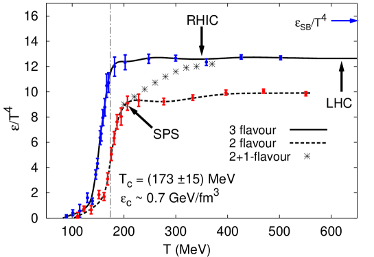
Figure 1.1: Energy density as a function of temperature calculated in lattice QCD at zero baryon chemical potential with various numbers of degenerate quark flavors [10].

In the lattice calculations a discontinuity in the energy density as a function of temperature is found at a critical temperature of the order of $T_{c}\approx$170 MeV, corresponding to an energy density of $\epsilon\approx$1 GeV/fm³ [10], Figure 1.1. There are however many uncertainties involved regarding the actual value of this temperature, and the order of the phase transition. The reason is that both depend on the number of flavors and the bare quark masses being used in the calculations. In the high temperature and zero baryon density limit, the phase transition is fully described by the chiral symmetry of the QCD Lagrangian [11]. This symmetry is a global intrinsic symmetry of the theory which is exact only in the limit of vanishing quark masses. However, the quarks in nature are not massless, and in particular the heavy quarks (charm, bottom and top) are too heavy to play a role in the thermodynamics in the vicinity of the phase transition. However, the strange quark, whose mass is of the order of $T_{c}$, plays a crucial role in deciding about the nature of the transition at vanishing baryon density. In the massless limit a three flavor QCD shows a first order phase transition. Recent lattice calculations indicate that the phase transition for realistic values of the up, down and strange quark masses may even be a rapid crossover taking place in a narrow temperature interval around $T_{c}\sim$170 MeV [12].

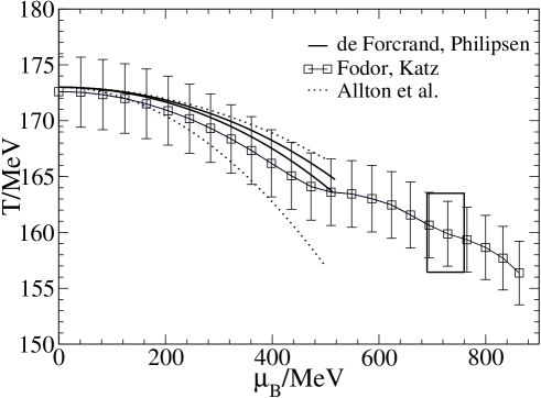
Figure 1.2: Lattice calculations at finite baryon chemical potential from [13] and references therein. The lines indicate a rapid crossover transition at low $\mu_{B}$ which becomes first order above the tri-critical point. The position of this point (indicated by the rectangle on the figure) is subject to significant uncertainties.

At finite baryon chemical potential ($\mu_{B}\neq$0) the standard Monte-Carlo sampling techniques used in lattice calculations, Figure 1.1, are no longer applicable. However, recent theoretical progress has overcome this problem, and consequently extends the lattice simulations of the QCD phase transition for values up to $\mu_{b}$=0.5-0.8 GeV [13], Figure 1.2. The results show a slight decrease of $T_{c}$ with increasing $\mu_{B}$.

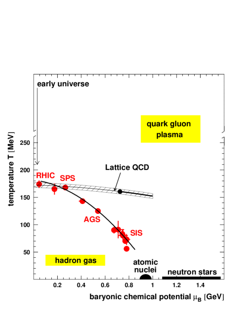
Figure 1.3: QCD phase diagram summarizing the present understanding about the structure of nuclear matter at different densities and temperatures. The points marks illustrates the results achieved by the different ultrarelativistic collider experiments, and the dashed line represent the lattice QCD calculations.

The present experimental and theoretical knowledge about the different phases of strongly interacting matter can be summarized in a generic QCD phase diagram, Figure 1.3. In addition to the phase transition at high temperatures, deconfinement is expected at sufficiently large density (several times normal nuclear matter density) and low temperature. However, in this case the evidence is less compelling due to the lack of lattice results for very high values of $\mu_{B}$.

Relativistic heavy ion collisions

Relativistic heavy ion collisions offer a unique tool to probe hot and dense nuclear matter in the laboratory. During the last decades a great number of experiments have been carried out in order to explore the nuclear state of matter as a function of temperature and energy density. The main motivation is the search for a QGP phase. At the CERN SPS accelerator a series of fixed target experiments has collected a wealth of information about nuclear matter at center-of-mass energies of $\sqrt{s}$=5-20 A GeV. However, the results have not firmly established the existence of the QGP phase yet, as the energy density obtained only slightly exceeds the critical temperature, $T_{c}$.

Current heavy-ion experiments at the Relativistic Heavy Ion Collider (RHIC) at Brookhaven National Laboratories (USA) and scheduled experiments at the Large Hadron Collider (LHC) at CERN (Switzerland), will generate sufficiently high energy densities to form a baryon-free plasma. At the RHIC accelerator, four experiments are dedicated to the study of Au–Au collisions at center-of-mass energies up to $\sqrt{s}$=200 A GeV. Furthermore, the LHC will make Pb–Pb nuclei collide at $\sqrt{s}$=5.5 A TeV which will be studied by the ALICE experiment. At these energies, nuclear matter is predicted to be transparent enough to form baryon-free matter, heated well beyond the expected phase transition temperature.

1.3 The dynamics of heavy ion collisions

Even though relativistic heavy ion experiments in the laboratory may recreate the conditions for a phase transition, direct comparison to lattice QCD calculations is generally very difficult. The reason is that lattice QCD exclusively describes matter in a thermodynamical equilibrium, while the outcome of a heavy ion collision is a finite, highly excited and dynamical non-equilibrated system. The correct theoretical treatment of such a system is therefore not a trivial task, and involves concepts which go far beyond the capabilities of simple statistical thermodynamics. These models can however be valuable as they can provide first order (quasi-)analytic solutions that can be compared directly with measured quantities.

The evolution of a heavy ion collision in space and time depends extensively on the initial conditions of the system. Consequently, heavy ion collisions are generally divided in two energy domains: Lower energies where the stopping power is sufficient to stop the colliding nuclear matter, and higher energies, where the colliding baryons initially penetrate each other. The former case is applicable to the energy range of the AGS and SPS experiments, and is commonly described within Landau’s fluid-dynamical model. For the energies which will be obtained at the LHC, the latter scenario is most likely to be the case, and is often described with the scaling hydrodynamical model of Bjorken [14], Figure 1.4. In this picture, the Lorentz contracted nuclei become almost completely transparent to each other, and the valence quarks maintain their initial rapidities. At their inter-penetration, however, the partons interact creating a high energy density chromo-electric field between the two nuclei. Within the chromo-electric field a system of non-equilibrated deconfined quarks and gluons is created. This matter constitutes the so-called pre-equilibrium phase, which after a certain formation time might lead to a local thermal equilibrium provided that there are enough interactions among the constituents. The initial conditions at which an equilibrium is reached is defined by the proper time, $\tau$. The proper time is defined as the local time in the rest frame of any fluid element. If all the particles originate from one point in space-time the proper time can be expressed as

$$\tau=t/\gamma=\sqrt{t^{2}-z^{2}}.$$

After a formation time $\tau_{0}$ which is likely to be 0.5 to 2 fm/c the system reaches thermal equilibrium which is characterized by a uniform energy density and temperature. From that time on the system is treated using 1+1 dimensional (spatial + time) ideal relativistic fluid dynamics, where the system expands in the longitudinal direction.

As the system expands, the equilibrated plasma of deconfined quarks and gluons quickly cools down to the temperature where a phase transition into a hadron gas takes place. Depending on the type of the transition, the system may spend some time in a mixed phase where the QGP coexists with the hadron gas. Finally, the size of the system becomes larger than the mean free path of hadrons, in which they undergo a freeze-out and stream freely towards the detectors. This freeze-out process is most usually treated as a sudden freeze-out, implying that at a given instant in the space-time all constituents within the fluid become independent, and final interactions and collisions are neglected.

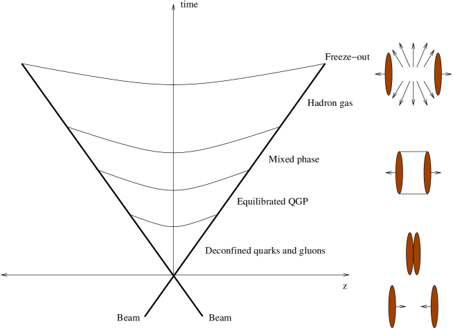
Figure 1.4: The Bjorken space-time scenario for a heavy ion collision. The two colliding nuclei resembles two flat discs because of the Lorentz contraction in the laboratory frame. The parabola indicate the constant proper times.

1.4 The experimental observables

In order to establish experimentally the properties of the hot and dense partonic matter created in heavy ion collisions, a wide range of variables of the system have to be measured. Due to the short existence and limited spatial extend of the generated plasma, however, basic properties such as volume, temperature, density of the plasma state and the masses of the quarks contained in it, cannot be measured directly. Instead, it must be derived from the remnants of the collision, i.e. the final state particles which after the freeze-out-stage has reached the detectors. Several observables have been suggested and identified, which needs to be evaluated individually and/or in combination with other probes.

In general, the observables in a heavy ion collisions can be divided into three main categories:

• Hadronic observables.

• Electromagnetic observables.

• Hard probes.

Each of the observables are characteristic of a certain stage in the collision, but they are not completely independent of each other. The hadrons emerge only in the final stage of the collision after they freeze-out from the hadron gas, and thus carry information about the system at the time of freeze-out. The electromagnetic observables on the other hand will, because of their long mean-free-path relative to the size of the QCD medium, manage to escape from the system without any further interaction, and thus emerge predominately from the earlier, hot stage of the collision. Lastly, the initial stage of the collision is dominated by the collision dynamics of the produced partonic system, and the study of hard processes enable to probe the very early parton dynamics and evolution of the initial stage of the system.

In the following the main observables which will be relevant at LHC energies, and therefore will be measured by the ALICE experiment, will be introduced. These observables are based on theoretical predictions combined with experimental results from SPS and RHIC.

Hadronic observables

The hadronic observables are often referred to as soft probes of the heavy ion collision, as they mostly connect to the non-perturbative aspects of QCD. They deal with the more global characteristics of the system such as particle production, particle abundances and spectra and correlations.

Particle multiplicity

One of the most important and fundamental observable in a heavy ion collision is particle multiplicity. By measuring the number of particles produced in the collision, one can determine the energy density of the system. From a theoretical point of view, this is important since it enters the calculation of most other observables. On the experimental side, the particle multiplicity fixes the detector performance, and thus the accuracy with which many of the observables can be measured.

The particle multiplicity in heavy ion collisions is very difficult to predict, since it cannot be calculated from first principles.

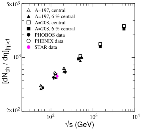
Figure 1.5: Data and predictions for charged particle multiplicity per unit pseudo-rapidity [15].

The obvious approach is thus to extrapolate already measured quantities obtained in lower energy experiments, using different theoretical extrapolation models. In Figure 1.5 data from RHIC and predictions for center of mass energies up to LHC levels ($\sqrt{s}$=5.5 TeV) [15] are shown. At RHIC the charged particle multiplicity per unit pseudo-rapidity, dN_ch/d$\eta$, is measured to be 700-800 at $\eta$=0. The predictions for LHC show that one should expect a value of about 2200. In [16] the multiplicity is computed in a two-component soft+semi-hard string model, which gives a slightly higher density of 2600-3200, depending on the initial assumptions.

Particle spectra and correlations

Most of the particles emitted in a heavy ion collision are hadrons which decouple from the collision region during the hadronic freeze-out stage. Hence, by measuring the different particle spectra, one obtains information about the chemical and kinetically freeze-out distributions. From these observables, one can derive quantities like the freeze-out temperature and chemical potential, flow velocities within the expanding system, size of the system etc. Since these distributions are also highly constrained by the dynamical evolution of the system, they will also yield information about the early stages of the collision [17, 18, 19]. Furthermore, the final momentum distributions may provide detailed information about the time evolution of the collision system [20].

Essential information about the collision system is obtained from studying its evolution in time and space. The size and expansion results from the work of pressure gradients within the system, and hence reflects directly the underlying equation of state. This can be obtained directly by particle interferometry or correlations. By these methods one can measure the final size of the fireball, gain insight about its expansion and phase-space density and provide information about the timing of the hadronization.

Furthermore, the so-called elliptic flow is sensitive to the degree of thermalization achieved in the system. In general it describes the azimuthal asymmetry of the particle production, and builds up through re-scattering in the evolving system which converts the spatial anisotropy into momentum anisotropy. A rapid expansion of the hot system will destroy the original anisotropy and reduce the following momentum anisotropy. Thus by measuring the elliptic flow, information about the early stage of the collision is obtained, and in particular whether local thermalization is reached followed by a collective hydrodynamic expansion. The observed large elliptic flow measured at RHIC, Figure 1.6, indicates that the hydrodynamical model is applicable for a wide range of momenta and particle types.

     

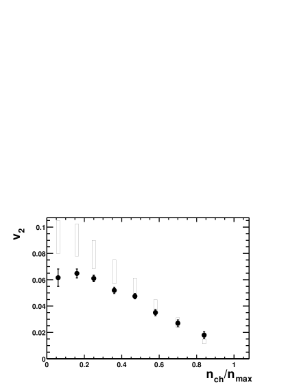
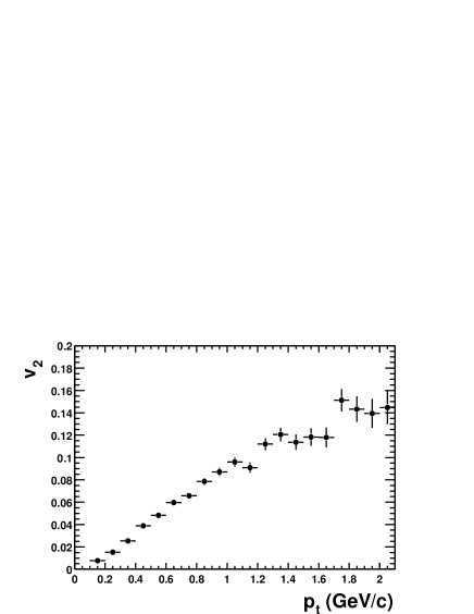
Figure 1.6: Measured elliptic flow at RHIC [21]. Left: Elliptic flow as a function of centrality. The open rectangles show a range of values expected in the hydrodynamical limit. Right: Elliptic flow as a function of transverse momentum for minimum bias events.

Fluctuations

Like any other physical measured quantities, the observables in a heavy ion collisions are also subject to fluctuations. These fluctuations can themselves provide useful information about the collision as they are generally system dependent. One of these observables is the fluctuation of certain particle ratios, as they give access to information about the abundance of resonances at the chemical freeze-out [22]. Furthermore, by measuring the charge fluctuations per unit degree of freedom of the system in a heavy ion collision, one can gain knowledge whether a QGP phase was created [23]. The argument is that in a QGP phase the system would consist of quarks and gluons which means that the unit of charge is 1/3, while in a pure hadronic phase it will be 1. The fluctuation in the net charge depends on the squares of the charges, and hence are strongly dependent of the phase it originates from.

Electromagnetic observables

Electromagnetic observables, like photons, carry unperturbed information about the source in which the photons have been produced. Since photons are electromagnetically interacting particles, their mean free path in the QCD medium is large enough to escape the system without any further interaction. These so-called direct photons provide a powerful probe of the evolution of the collision. However, the experimental feasibility is dominated by a severe background from the radiative decay of neutral pions ($\pi^{0}\rightarrow\gamma\gamma$). Results from WA98 experiment indicates that the task of extracting the direct photons at SPS-energies is feasible [24]. Recent results from the PHENIX experiment at RHIC show a direct photon signal above the expected background in central Au–Au events [25].

Hard probes

During the initial non-equilibrated stage of a heavy ion collision at LHC, the dynamics are dominated by hard processes within the interacting partonic system. The study of such processes thus probes the very early parton dynamics and the evolution of the QGP phase. In contrast to the hadronic observables, the hard probes involve only a limited number of energetic colliding partons, and are theoretically treated by perturbative QCD.

Jet production

During the inter-penetration of two high energetic colliding nuclei, the partons within the projectiles interact with each other in hard 2 to 2 processes, and the initial parton momentum is transferred into final state partons or photons. Each of these final state partons will then emerge back-to-back from the collision region and radiate energy because of their color charges before they finally hadronize into a number of colorless hadrons. The resulting cluster of particles is commonly referred to as jets.

High transverse energy jets produced in a heavy ion collision are expected to loose major parts of their initial energy when traversing the collisions region prior to the freeze-out phase. Studying jet production can thus help to determine the QCD medium effects acting on a color charge traversing a medium of color charges, in analogy to the Bethe-Bloch physics of QED. By comparing the cross section for jet production for that in p–p collisions at the same center of mass energy, one can identify these medium modifications of the jet properties which characterize the hot and dense nuclear matter in the initial stage of the collision region.

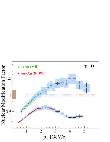
Figure 1.7: Nuclear modification factor measured for minimum biased collisions of d–Au at $\sqrt{s_{NN}}$=200 GeV compared to central Au–Au collisions [26]. The nuclear modification factor is defined as the ratio of the hadron yields in nucleus-nucleus interactions and the yield in nucleon-nucleon interactions scaled by the equivalent number of binary nucleon-nucleon collisions to account for the collision geometry.

Several observables has been proposed as probes for the energy loss of the fast moving partons in the medium of deconfined color charges [27, 28, 29]. In particular, this energy loss should be visible as a reduced yield, or quenching, of high momentum hadrons in central A-A collisions. This effect has indeed been observed at RHIC, Figure 1.7. The measurements show that central collisions between Au–Au nuclei exhibit a very significant suppression of the high transverse momentum component as compared to nucleon-nucleon collisions. This observation indicates a substantial energy loss of the final state partons or their hadronic fragments in the medium generated by high energy nuclear collisions.

Furthermore, the production of jets has been demonstrated in angular correlations of high transverse momentum hadrons through the observation of enhanced correlations at $\Delta\phi\sim 0$ and $\Delta\phi\sim\pi$, Figure 1.8. By comparing the measurements from d–Au collisions to central Au–Au collisions one observes a suppression of the back-to-back correlation for central Au–Au collisions, indicating that one of the two jets is no longer present. If this suppression would be a result of initial-state effects, it should consequently also be observed in d–Au collisions but no such suppression is observed. This energy imbalance thus suggests that one of the jets which has a much longer in-medium path-length interacts with the dense system and looses substantial amounts of its energy, which is in agreement with the predicted jet quenching in a QGP.

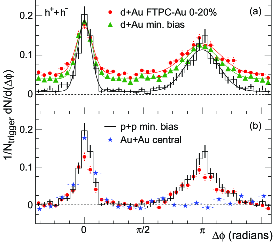
Figure 1.8: Two-particle azimuthal distributions for high transverse momentum hadrons measured at RHIC [30]. The distributions in d–Au collisions include a near side ($\Delta\phi\sim 0$) peak similar to that seen in p+p and Au–Au collisions and typical of jet production, and a back-to-back ($\Delta\phi\sim\pi$) peak similar to di-jet events seen in p+p. This second peak is suppressed in central Au–Au collisions, indicating final state interactions with the dense system generated in the collision.

Heavy quark production

Heavy quarks like charm and bottom provide a probe which is highly sensitive to the collision dynamics. Heavy quark production is an perturbative phenomenon which takes place on a time scale of the order of the inverse quark mass. The relative long lifetime of the charm and bottom quarks allows them to live through the thermalization phase of the QGP, and thereby also be affected by its presence. Also, heavy quark-anti-quarks may form quarkonium states with binding energies comparable to the temperature of the QGP, implying a large quarkonium break-up and suppression.

Typical observables including heavy quark production are the total production rates, transverse momentum distributions and kinematic correlations between the heavy quark and anti-quark. These observables have to be compared to those of p–p and p–A collisions in order extract information on the properties of the hadronic plasma.

The observables connected to the heavy quark production will become increasingly important at LHC energies, as the center of mass energy will be sufficient to copiously produce the heavy quarks charm and bottom and their bound states.

Chapter 2 The ALICE Experiment at LHC

2.1 Introduction

The LHC accelerator at CERN is scheduled for 2007. As the only experiment build for the heavy ion program, the A Large Ion Collider Experiment (ALICE) experiment is optimized for the study of heavy ion collisions at the foreseen center of mass energy of $\sim$5.5 A TeV. The main goal of this experiment is to probe in detail the non-perturbative aspects of QCD such as deconfinement and chiral symmetry restoration. Extrapolating from present results, all parameters relevant to the formation of the QGP phase will be more favorable, and in particular the energy density and the size and lifetime of the system should all improve by an order of magnitude compared to SPS and RHIC.

The ALICE detectors are designed to measure most of the observables which is relevant to the formation of a QGP phase. The experimental capabilities to measure these observables depend both on the performance of the detectors and the number of events which can be collected.

2.2 LHC running strategy

The heavy ion program foreseen for LHC will mainly consist of two parts [31]: Colliding Pb–Pb at the highest possible energy, and a more limited systematic study of different collision systems for different beam energies. In addition to A–A systems, both p–p and various p–A systems will be studied in order to study the system as a function of energy density and to provide reference data for the Pb–Pb systems. The ALICE running program has therefore been divided into two phases: An initial phase which is based on the current theoretical understanding and results from RHIC, and a second phase where a number of different running options will be considered depending on the outcome of the initial results.

The first data that will be taken with ALICE will be from p–p collisions. The LHC will start running with several months of proton beams, followed by the end of each year by several weeks of heavy ion collisions. The effective running time per year is expected to be 10⁷ s for proton and 10⁶ s for heavy ion operation. During the first heavy ion run, Pb–Pb collisions at the highest energy density is foreseen to provide global event properties and large cross section observables. For low cross section observables, and in particular hard processes which are the main focus of LHC, 1-2 years of Pb–Pb runs at the highest possibly luminosity are required to collect sufficient amount of statistics. In the later running phase, p–Pb collision will be run in order to provide reference data for Pb–Pb systems. Further on, energy dependencies will be studied by using lower-mass ion systems such as Ar–Ar.

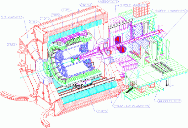
Figure 2.1: The ALICE detectors.

2.3 Detector layout

The complete layout of the ALICE detector as proposed initially together with the physics objectives are described in the ALICE Technical Proposal [32, 33, 34]. Since then, some of the sub-detectors have been modified to meet the new experimental goals set by the most recent results from RHIC and latest theoretical developments. Most of the individual sub-detectors are described in detail in their respective technical design reports [35, 36, 37, 38, 39, 40, 41, 42, 43, 44, 45]. In the following a brief description of the general ALICE detector layout and a introduction to the different sub-systems, is given.

The experimental setup of the ALICE detectors, Figure 2.1, is mainly composed by three parts:

• The central barrel which is contained in the L3 magnet. The detectors in the central barrel region have an acceptance in pseudo-rapidity of $|\eta|<$ 0.9 over the full azimuth angle. These detectors will probe hadronic signals, di-electrons and photons.

• The forward muon spectrometer for detecting muon pairs from the decay of heavy quarkonium in the interval 2.5 $<\eta<$ 4.0.

• The forward detectors, $\eta>$ 4, which will be used to determine the multiplicity. These detectors will also be used as a fast centrality trigger.

The Inner Tracking System

The Inner Tracking System (ITS) is designed and optimized for reconstructing secondary vertices from hyperon and charmed meson decays, and precision tracking and identification of low $p_{t}$ particles. The detector consists of 6 layers of high resolution silicon detectors, located at innermost radius 4 cm to outermost 44 cm. The different layers are designed to achieve an impact parameter resolution of 100 $\mu$m within the expected particle density. Hence the innermost layers consists of pixel detectors, silicon drift detectors for the following two, and the two outer layers are equipped with double-sided silicon micro-strip detectors.

The Time Projection Chamber

The main tracking device in ALICE is a cylindrical Time Projection Chamber (TPC). Its main purpose is thus to provide charge particle momentum measurement over the central rapidity region and particle identification via dE/dx. In addition, it will use information from the ITS, Transition Radiation Detector (TRD) and Time Of Flight (TOF) detector (see next section) in order to obtain a more accurate vertex determination, particle identification and two track separation. The TPC has an inner radius of 90 cm which is given by the maximum acceptable hit density, and an outer radius of 250 cm defined by the length required for a dE/dx resolution of $<$10%. The overall acceptance is $|\eta|<$ 0.9 and thus matches that of the ITS, TRD and TOF.

Detectors for Particle Identification

Particle identification (PID) for a large part of the phase space is obtained by a combination of dE/dx from the ITS and TPC, and time of flight information from the Time of Flight (TOF) detector.

Electron identification above 1 GeV/c is provided by the Transition Radiation Detector (TRD). The TRD will in conjunction with ITS and TPC provide electron identification in order to measure, in the di-electron channel, the production of light and heavy meson resonances as well as to study the di-lepton continuum.

For the high momentum PID a Ring Imaging Cherenkov (RICH) detector will be used. The detector covers 5% of the acceptance of the central detectors, and allows PID of hadrons up to 5 GeV.

The Photon Spectrometer

The measurement of direct photons, $\pi^{0}$ and $\eta$ is provided by a high-resolution electromagnetic calorimeter, the Photon Spectrometer (PHOS). The detector is located on the bottom of the ALICE experimental assembly, and is built from scintillating lead-tungstate crystals coupled with photo-detectors. The readout electronics provides both energy and time information to reject anti-neutrons and trigger for high $p_{t}$ photons.

The Muon Arm

The forward muon spectrometer will allow study of vector resonances via the $\mu^{+}\mu^{-}$ decay channel. It is placed outside the L3 magnet, and consists of a composite absorber close to the interaction point in order to reduce the $\mu$ background from $\pi$ and $K$ decays. The spectrometer magnet is a large dipole magnet with a nominal field of 0.7 T. Tracking is performed within 10 planes of thin multi-wire proportional chambers with cathode readout.

The Forward Detectors

Several smaller detectors placed in the forward region, $\eta>$4, will be used to measure global event characteristics such as the event reaction plane, multiplicity of charged particles and precise time of the collision. The multiplicity information is partially used to derive a trigger.

A set of four small and very dense calorimeters, the Zero Degree Calorimeter (ZDC) will be used to measure and trigger on the centrality of the collisions.

The Photon Multiplicity Detector (PMD) is a pre-shower detector which is mounted behind the TPC opposite to the muon arm. It will measure the ratio of photons to charged particles, the transverse energy of neutral particles, the elliptic flow and the event reaction plane.

The Forward Multiplicity Detector (FMD) consists of silicon pad detectors organized in five disks which is placed on both sides of the central detectors. It will measure the pseudo-rapidity distribution of charged particles over a large fraction of the phase space.

The T0 counters are 24 Cherenkov radiators and will provide the event time with a precision of 50 ps. The V0 counters (consisting of scintillators) will be used as the main interaction trigger and to locate the event vertex.

2.4 The TPC detector

The ALICE TPC detector is the main tracking device. It is placed inside the homogeneous magnetic field of the L3 magnet. With almost full three dimensional coverage, the tracking detector can provide information of the complete particle track in addition to the particles specific energy loss, dE/dx. Experience from previous experiments show that TPC detectors can handle high particle multiplicities and high track densities (EOS [46], NA49 [47] and STAR [48]).

2.4.1 Principle of operation

The TPC detector is a gaseous ionization detector. This group of detectors are sensitive to the ionization electrons and ions that are produced when charged particles traverse the gas in the detector.

The TPC detector consists of a large cylindrical chamber filled with gas, Figure 2.4. A uniform electric field, E, is applied and directed along the detector volume. When charged particles traverse the gas they will ionize the gas along their trajectory liberating electrons. The liberated charge is subject to the electric field, and electrons will drift opposite the direction of E towards the end-caps of the chamber where their position is detected. This then yields the two-dimensional position of a space point onto the end-cap plane. The third coordinate is given by the drift time of the ionization electrons. Since all ionization electrons created in the sensitive volume of the TPC will drift towards the end-cap, almost a continuous sample of space points for each track is detected allowing a full reconstruction of the particle trajectory. Furthermore, the charge which is collected at the end-caps is proportional to the ionization, and thus the energy loss, of the particle. The signal amplitudes provide information on dE/dx of the traversing particle. In conjunction with the measured momentum obtained from the curvature of the trajectory in the magnetic field, this enables particle identification.

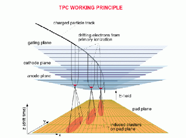
Figure 2.2: TPC principle for detection of charged particle trajectories.

The detection of the drifting electrons is done by using Multi-Wire Proportional Chambers (MWPC), Figure 2.2. The primary electrons by themselves do not induce a sufficiently large signal for readout. The necessary signal amplification is provided by avalanche creation in the vicinity of anode wires. The readout chambers consist of a grid of anode wires above a cathode pad plane, a cathode wire grid and a gating grid. A negative voltage is applied to the cathode wires and cathode pads producing an electric field near the anode wires with a 1/r dependence. When the drifting electrons enters the region behind the gating grid, they will continue to drift along the field lines towards the nearest anode wire. Upon reaching the high field region close to the anode wire, the electrons will be accelerated to produce an avalanche. The positive ions liberated in the avalanche process will induce charge on the cathode pads. This signal current is characterized with a fast rise time and a long tail due to the motion of the positive ions.

The function of the gating grid is to open and close the amplification region to the drift volume. When a trigger signal is issued, the gating grid wires are held at the same potential, admitting the electrons from the drift volume to enter the amplification volume. Then, when absence of a valid trigger, the gating grid is biased with a bipolar field which prevents the electrons from drifting into the avalanche region. In addition, the closed gate prevents the positive ions created in the previous event from drifting back into the drift volume. This is important since escaping ions into the drift volume accumulate, and can cause severe distortions of the drift field.

A precise measurement of the location of the avalanche can be obtained if the induced signal is distributed over several adjacent readout pads, using an appropriate center-of-gravity algorithm. The position of the particle track in the drift direction can be determined by sampling the time distribution of each pad signal. The resulting two-dimensional pulse height distribution in pad-time space is called a cluster.

Signal shape and position resolution

The intrinsic resolution of a TPC detector is determined by the so-called Pad Response Function (PRF). This function represent the relative pulse height distribution of signals induced on adjacent pads by a point-line avalanche. Its distribution is well approximated by a Gaussian function,

$$P_{i}=C\cdot\exp\left(\frac{(x-x_{i})^{2}}{2\sigma_{x}^{2}}\right),$$ (2.1)

where $x$ is the position of the induced avalanche and $x_{i}$ the respective pads. The width of the distribution, $\sigma_{x}$, is not entirely determined by the PRF. The reason is that the drifting electrons are spread because of diffusion when drifting towards the end-caps. Thus, the distribution of the primary electrons arriving at the anode wires cannot be considered point-like. In addition, the finite track inclination angle with the pad-plane spreads the ionization such that width of the initial charge distribution represents a projection of the track segment over the pad-length. The resulting mean cluster width along the pad-direction can be parameterized as [49],

$$\sigma_{x}^{2}=\sigma_{PRF}^{2}+D_{t}^{2}\cdot s_{\mathrm{drift}}+\frac{l^{2}\cdot\tan^{2}(\beta)}{12}+\frac{d^{2}\cdot(\tan(\alpha)-\tan(\psi))^{2}}{12}$$ (2.2)

where $D_{t}$ is the diffusion constant of the gas, $s_{\mathrm{drift}}$ is the drift distance of the drifting electrons, $l$ is the pad-length, $d$ is the distance between two anode wires and $\beta$ is the inclination angle of the track, Figure 2.3. The angle between the normal to the anode wires and the projection of the track, $\alpha$, is in the ALICE TPC equal to $\beta$. The Lorentz-angle, $\psi$, is defined as the angle between the electric field and the drift-velocity. This angle applies near the anode wires where the electric and magnetic fields are no longer parallel, leading to a displacement of the drifting electrons.

Figure 2.3: Definition of the track inclination angle in the ALICE TPC.

In the longitudinal direction, the width of a pad signal generated by a single electron avalanche is given by the shaping constant of the readout electronics. The time signal is obtained by folding the avalanche with a Gaussian shaping function. Also in this direction the electron distribution suffers from diffusion and track inclination, and similar to Equation 2.2 the mean cluster width in the longitudinal direction can be parameterized by

$$\sigma_{L}^{2}=\sigma_{0}^{2}+D_{l}^{2}\cdot s_{\mathrm{drift}}+\frac{l^{2}\cdot\tan^{2}(\lambda)}{12},$$ (2.3)

where $D_{l}$ is the longitudinal diffusion constant, and $\lambda$ is the inclination angle of the track in the drift direction.

The cluster widths are subject to fluctuations, which depends on the contribution of the random diffusion and the angular spread, and on the gas gain fluctuation and secondary ionization. Furthermore, deviations from the Gaussian shape of the clusters may occur as a result of asymmetric distribution of the electron cluster.

The accuracy in which the centroid of the cluster can be determined is limited by the spread of the ionization and the subsequent diffusion which amplifies this spread. Similar to the widths of the cluster, the resolution therefore also depends on the track inclination angles and the drift distance, and is theoretically given by [49]:

$$\delta_{x}^{2} = \delta_{x,0}^{2}+\frac{D_{t}^{2}\cdot s_{\mathrm{drift}}}{l\cdot n_{e}}+\frac{l^{2}\tan^{2}(\beta)}{12\cdot n_{\mathrm{eff,pad}}}+\frac{d^{2}\cdot(\tan(\alpha)-\tan(\psi))^{2}}{12\cdot n_{\mathrm{eff,wire}}\cdot n_{\mathrm{sense}}}$$

$$\delta_{y}^{2} = \delta_{y,0}^{2}+\frac{D_{l}^{2}\cdot s_{\mathrm{drift}}}{l\cdot n_{e}}+\frac{l^{2}\tan^{2}(\lambda)}{12\cdot n_{\mathrm{eff,pad}}}$$ (2.4)

Here, $n_{e}$ is the number of ionized electron-ion pairs per cm track length, $n_{\mathrm{eff,pad}}$ is the number of primary electrons in the gas “column” below the pad, $n_{\mathrm{eff,wire}}$ is the number of primary charged units along an anode wire on which the cluster charge is deposited and $n_{\mathrm{sense}}$ is the number of anode wires crossing the pad.

Occupancy

The performance of a TPC depends highly on the detector occupancy. The occupancy is a measure of the track density with respect to the intrinsic detector resolution. In general, one can define it as the probability of having a signal above threshold,

$$O=\frac{N_{\mathrm{above}}}{N_{\mathrm{all}}},$$ (2.5)

where $N_{\mathrm{above}}$ is the number of signals above threshold and $N_{\mathrm{all}}$ is the total number of time-bins. For the TPC, the signals are the bins in pad-row-plane. The number of active signals is a function of the particle density, $F$,   and on the effective cluster area, $s_{\mathrm{eff}}$, and can be expressed as

$$O=1-\exp(-F\cdot s_{\mathrm{eff}})$$ (2.6)

Since the occupancy is a function of effective cluster area, an optimization of the detector parameters in terms of cluster widths is necessary. As described above the cluster widths in general depends on diffusion, response functions and on the pad-length. For a given gas and drift field the diffusion is no longer a variable factor, and the cluster size is thus determined by the geometry of the pad.

2.4.2 Detector layout

The overall design of the ALICE TPC detector consists of a cylindrical chamber with an inner radius of $\sim$90 cm, an outer radius of $\sim$250 cm, and a length of $\sim$500 cm, Figure 2.4. A thin high voltage electrode divides the cylinder in two, and provides a uniform electric drift towards the end-caps. The readout chambers which cover the end-caps of the TPC cylinder, consist of conventional MWPC with cathode pad readout. The azimuthal segmentation of the readout plane follows that of subsequent ALICE detectors, which leads to 2$\times$18 (both sides of the TPC) trapezoidal sectors, each covering 20^∘ in azimuth.

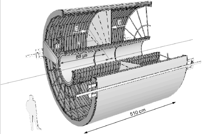
Figure 2.4: ALICE TPC schematic layout.

The overall acceptance covered by the TPC is $|\eta|<$ 0.9 for full radial track length, and to about $|\eta|<$ 1.5 for reduced track lengths and poorer momentum resolutions.

The detector parameters are chosen to minimize the detector occupancy under the expected high track density. Based on calculations of the PRF for different pad and wire geometry, a rectangular pad shape has been chosen for the ALICE TPC, Figure 2.3. Because of the cylindrical volume of the ALICE TPC, the track density has a radial dependency and is proportional to $r^{-2}$. This leads to different requirements for the pad sizes and the corresponding readout chambers as a function of distance from the interaction point. Therefore, the readout is segmented radially into two separate readout chambers with slightly different wire geometry and pad sizes. In total there are 557 568 readout pads of three different sizes, Table 2.1.

	Inner chambers	Outer chambers
Pad size	4$\times$7.5 mm	6$\times$10 mm	6$\times$15 mm
Total number of pad-rows	63	64	32
Total number of pads	5504	4864	5120

Table 2.1: ALICE TPC design parameters of the readout chambers [31].

The radial distance of the active area is from 84.1 cm to 132.1 cm and from 134.6 cm to 246.6 cm for the inner and outer chambers respectively, while the total area is 32.5 m².

The drift gas is optimized for drift speed, low diffusion, low radiation length and hence multiple scattering, small space-charge effect and aging properties. The parameters related to the gas and the drift field is listed in Table 2.2.

Detector gas	Ne/CO2 (90/10)
Gas volume	88 m3
Drift length	2$\times$250 cm
Drift field	400 V/cm
Drift velocity	2.84 cm/$\mu$s
Drift time	88 $\mu$s
Total HV	100 kV
Diffusion	220 $\mu$m/$\sqrt{\mathrm{cm}}$

Table 2.2: ALICE TPC design parameters of the gas volume [31]. The choice of gas mixture is currently under discussion, and may also include N₂.

2.4.3 Readout

The front-end electronics of the detector is responsible for reading out the charge induced on each of the cathode pads. Each of these readout channels is comprised of three basic units [50]: A charge sensitive PreAmplifier/ShAper (PASA), a 10-bit Analogue to Digital Converter (ADC), and a digital signal processing circuit.

The charge induced on a pad is amplified and integrated by the PASA. A single channel is designed to have a noise value (r.m.s.) $\leq$1000$e$. Immediately after the PASA, the 10 bit ADC samples the signal at a rate of 5-6 MHz. The digitized signal is then processed by a set of circuits contained in a single chip named ALTRO (ALice Tpc ReadOut). Each ALTRO contains 16 channels that operate concurrently to digitize and process the input signals. Baseline shifts due to signal pile-ups are removed. After the processing, the ALTRO chip performs zero-suppression. Zero-suppression means that a base-line ADC-value corresponding to 2-3 times the RMS-value above noise is subtracted to correct for signal baseline instabilities. Hence, ADC-values smaller than a preset constant threshold value are rejected. In addition, a filter checks for a consecutive number of samples above the threshold in order to identify the sequences corresponding to the pulses. The zero-suppressed data are then formatted into 32-bit words according to a back-linked data structure. The ALTRO also contain a multiple-event buffer for storing trigger-related data. When a L1 trigger signal is received (Section 2.5.2), the data is stored in memory, and upon arrival of the second level trigger (L2 accept or reject) the latest event in the data stream is either frozen in the data memory until complete readout takes place, or discarded.

The complete readout chain is contained in the Front-End Cards (FEC) plugged into crates and attached directly to the detector. Each FEC contains 128 channels and is connected to the cathode readout plane by means of 6 cables. A number of FECs are controlled by a Read Control Unit, which interface the FECs to the DAQ, the trigger system and the Detector Control System (DCS). The data is shipped to the DAQ using optical fibers called Detector Data Link (DDL). Each of the 36 TPC sectors are read out by 6 RCUs and 6 corresponding DDLs.

2.5 Data volumes and data-acquisition

2.5.1 Data rates

The data rate produced by the detectors is a function of both event rate and event data size. The event rate is given by the running luminosity, while the event data size is defined by the granularity of the detectors and the particle multiplicity. The maximum usable luminosity is limited by both the LHC accelerator and the detector dead times. Given the amount of readout channels the biggest amount of data is by far produced by the TPC detector.

Event rates

From a detector point of view, the maximum usable luminosity is limited by the the time it takes to read out the detectors. In particular, the TPC detector, which is the slowest detector, needs $<$90 $\mu$s for the electrons to drift to the end-caps. If the luminosity is high enough, additional events may occur within TPC frame during readout causing several superimposed events which are shifted in the time direction. These pile-up events will contribute to the track density and the detector occupancy, and consequently may lead to a loss in tracking performance. At an average luminosity of 10²⁷ cm^-2 s^-1, the minimum bias rate for Pb–Pb is 8 kHz for a hadronic interaction cross section of 8 barn, giving a probability of having a double event within the TPC frame of 76% [31]. The remaining “single” minimum biased Pb–Pb event rate is thus limited to 2 kHz, and the central event rate to 200 Hz.

In the case of p–p runs the situation is different. A single p–p event has a very low multiplicity compared to Pb–Pb, thus the TPC can tolerate several pile-up events without suffering any significant loss of tracking performance. In order to keep the pile-up at an acceptable level, the luminosity during p–p runs will be limited to $\sim$3$\times$10³⁰ cm^-2 s^-1 which corresponds to an interaction rate of $\sim$200 kHz. At this rate, there will on average be $\sim$25 piled-up events in the TPC.

Furthermore, the maximum possible event rate for both minimum biased Pb–Pb and p–p interactions is limited by the maximum TPC gating frequency to approximately 1 kHz. Considering the luminosity, event pile-up conditions and the maximum TPC gating rate, estimates of the maximum event rates can be obtained, Table 2.3.

Event sizes

The event sizes for Pb–Pb interactions are directly proportional to the multiplicity produced in the collision. This makes them very difficult to calculate as the multiplicities are hard to predict. For Pb–Pb collisions at 5.5 TeV predictions range from 2000 to 8000 particles per unit rapidity for central Pb–Pb collisions at LHC [31], while extrapolation from RHIC gives values around 2000-3500 (Section 1.4, page 1.4). During the design of ALICE the value 8000 was used as a baseline in order to provide a safety margin on the detector performance.

Simulations [35] indicate that the average TPC occupancy will be about 25% for the highest multiplicity. Multiplying the number of readout channels with the number of time-bins and taking into account the 10 bit ADC dynamic range, this leads to an event size directly at the detector readout of  350 MB. The ADC conversion gain is typically chosen so that $\sigma_{\mathrm{noise}}$ corresponds to one ADC count. This means that the relative accuracy increases with the ADC-values, and is not needed for the upper part of the dynamic range. The ADC-values can therefore be compressed non-linearly from 10 to 8 bits leading to a constant relative accuracy over the whole dynamic range. By compressing the ADC-values from 10 to 8 bits, the event size will be reduced to about 290 MB. In addition, since it is problematic to resolve individual tracks that have a low $p_{t}$ and cross the TPC volume under small angles relative to the beam axis, a 45^∘ cone will be cut out of the data resulting in the rejection of all particles which are not in the geometrical acceptance of the outer detectors. This will reduce the data size further by a factor of 40%. Finally, after zero-suppression the raw event size is expected to be $\sim$75 MB. If running at the central Pb–Pb interaction rate of 200 Hz, this corresponds to a TPC data rate of $\sim$15 GB/s.

Regarding p–p interactions, the estimated TPC event size for a single p–p collision is approximately 60 kB. In this case one also has to take into account the additional data coming from the pile-up events. The total data volume, including the piled up events, is estimated to be of the order of 2.5 MB. This event size is estimated assuming a coding scheme for the TPC data well adapted to a low occupancy and without any data compression. If running at the foreseen maximum TPC rate of 1 kHz, this would produce a total data rate $\sim$2.25 GB/s. In Table 2.3 the expected event and data rates for the different interactions are summarized.

Collision	Event rate	Data rate (approx.)
p–p	1 kHz	2.25 GB/s
Min. bias Pb–Pb	1 kHz	22 GB/s
Central Pb–Pb	200 Hz	15 GB/s

Table 2.3: Expected ALICE event and data rates for the different LHC runs [31].

2.5.2 The trigger system

As described in Section 2.2, the ALICE experiment will operate under different beam conditions. The trigger system is responsible for selecting the different types of events and enable readout of the detector when certain criteria are met. The ALICE trigger system is foreseen to operate in three different levels [32]: Level 0 (L0), Level 1 (L1) and Level 2 (L2). These different levels correspond to criteria imposed from different detectors, where the selection criteria gets stronger as the trigger number increase. Correspondingly, the rates at which each trigger level is operated decreases at higher levels.

The L0 and L1 trigger are both fixed-latency triggers, which means that their rate is constant. The main difference between the two is that the different detectors need trigger decision to strobe the electronics at different times after the interaction. The main task of the L0 trigger is to signal that an interaction has taken place at the earliest possible time, which is after about 1.2$\mu$s. This trigger is based exclusively on the information from the T0 and V0 counters and checks for the following features:

1. The interaction vertex is close the the nominal collision point.

2. The forward-backward distribution of tracks is consistent with a colliding beam interaction.

3. The measured multiplicity is above a given threshold.

No strong centrality condition is made at L0, as non-central events giving di-muon triggers are also required. At L1 decision, which is made after about 6.5$\mu$s, more stringent centrality requirements are made. Its selection is based on information from the muon system, PHOS, and on the centrality detectors, FMD and ZDC. At this time all the remaining detectors are strobed. In particular, the TPC gate is opened which leads to the requirement that the L1 trigger can have a maximum frequency of 1 kHz.

During the drift time of the TPC ($\sim$100$\mu$s) the L2 decision is made. Based on the data extracted from the different trigger sub-detectors, more selective algorithms are applied (e.g. a mass cut on the di-muon system). Also, during this time a reset can be issued as a result of pile-up events (only when running with Pb–Pb interactions). Since the selection algorithms will differ in processing time, the latency of the L2 trigger is not fixed, but has an upper bound as defined by the TPC drift time. After the L2 trigger, the data are all read out from the front-end electronics into the DAQ and High Level Trigger system.

2.5.3 The DAQ system

The data acquisition system [51] is responsible for collecting the data from all the sub-detectors and assemble the sub-event data blocks into full event before sending the data to mass storage. The architecture of the system is based on PCs connected by a commodity network, most likely TCP over Gigabit Ethernet. The data transfer from the front-end electronics of the detectors are initiated by a L2 trigger accept. The data is then transferred in parallel from all sub-detectors using special optical links, called Detector Data Link (DDL), into the Local Data Concentrators (LDC) where the sub-event building takes place. Parallel to the DAQ, the data is also shipped to the High Level Trigger system by duplicating the data stream (Figure 3.2). The sub-events prepared by the LDCs are transferred to one Global Data Concentrator (GDC) where the full event can be assembled. The event building is managed by the Event Building and Distribution System (EDBS), which is a protocol running on all the machines (LDCs and GDCs). A GDC destination for a particular event is determined by the EDBS which communicates this decision to the LDCs. The fully assembled events are finally shipped to permanent storage for archiving and further offline analysis.

The DAQ system is designed to be flexible in order to meet the requirements for the different data taking scenarios. As the p–p interaction produce only data rate of 1/5 relative to Pb–Pb interactions, the requirement on the system is defined by the expected data rate from the heavy ion runs. In the heavy ion mode, two main types of events have to be handled. The first consists of central Pb–Pb events at a relatively low rate but with a large event size. The second one concerns the events containing a muon pair which has been reported by the trigger and is read out with a reduced detector subset, including the muon arm. Much higher trigger rates are required in the latter case, typically up to 1 kHz.

2.5.4 The High Level Trigger

In the ALICE Technical Proposal [32], the collaboration estimated that a bandwidth of 1.25 GB/s to mass storage would provide adequate physics statistics. As seen from Table 2.3 the expected data rate from the detector exceeds this number by an order of magnitude. This has lead to the proposal and inclusion of the ALICE High Level Trigger (HLT) system. The task of this system is to reduce the data rate to an acceptable level in terms of DAQ bandwidth and mass storage costs, and at the same time provide the necessary event statistics. This is accomplished by performing online processing of the data, allowing partial or full event reconstruction in order to select interesting events or sub-events, and/or to compress the data efficiently using data compression techniques. Processing the detector information at a bandwidth of 10-20 GB/s requires a massive parallel computing system. The functionality and architecture of the HLT system are topics of Chapter 3.

Chapter 3 The ALICE High Level Trigger System

3.1 The necessity of a High Level Trigger

The ultimate goal of the ALICE detector is to detect and investigate the QGP phase of nuclear matter. This task can only be solved by a coherent measurement of a wide range of observables from both peripheral to central heavy ion collisions. An essential part of this measurement is the collection of enough events in order to obtain sufficient statistics for the physics analysis. On the other hand, hard processes such as heavy quarkonium and jet production corresponds to relatively small cross-sections, and consequently one needs to consider a large number of events to provide the adequate statistics for these observables. The systematic analysis of such hard signals therefore calls for running the detector at the full available luminosity, which makes it necessary to consider all interactions at the full available central event rate of 200 Hz. However, as described in Section 2.5.1, the foreseen data rate in such a scenario exceeds the planned mass storage bandwidth by an order of magnitude. It is therefore necessary to introduce some kind of online data reduction into the output data stream. Such a reduction should as far as possible reduce the data readout rate to match the DAQ and mass storage bandwidth, and at the same time allow ALICE to acquire sufficient statistics for the different physic observables. This has lead to the preparation of the ALICE High Level Trigger (HLT) system, whose prime task will be to enhance event selectivity and/or reduction of the event size by partial or full online event reconstruction.

3.2 Functionality

Data reduction in ALICE can in general be accomplished in two ways:

• Event rate reduction

• Event size reduction

The first method implies that only a fraction of the available events are sent to mass storage. This option would also be used without any HLT system being present, as the readout rate coming from the detectors would have to be decreased in order to meet the data rate limitation of the mass storage. However, by introducing the HLT system, data can be processed online and event selections may be performed on the basis of physics observables. Thus, the introduction of the HLT system will enable an event rate reduction and at the same time improve the event statistics needed for the different physic programs. In the latter case, selections of Region of Interest (ROI) and data compression techniques can be used to reduce the event size itself and thus increase the possible event rate being sent to mass storage.

In both cases online processing of the data is required, requiring pattern recognition in order to reconstruct the event. In the following the two cases will be referred to as running in trigger mode and data compression mode, respectively. In this context trigger means selection or rejection of events or sub-events on the basis of a specific physics analysis. In the data compression mode, the chunk of data representing an (sub)event is compressed by applying appropriate data compression techniques.

3.2.1 Trigger mode

The HLT trigger running mode can be divided into two subclasses: Complete event selection/rejection, and Region Of Interest (ROI) readout. Both of them are based on the online identification of some predefined certain physical event. Depending on the topology of the trigger signals, either full or partial event reconstruction is required for this mode of operation.

Although the hard probes of QCD are rare, and at the same time require high statistics for a systematic study, they provide to a large degree the most topologically distinct tracking signatures in the TPC. Therefore, most of the online HLT trigger algorithms will be based on online tracking of the TPC data. Further refinement may also result from using early time information of the ITS and TRD systems. The different feasible trigger modes envisaged to date are described in detail in the HLT Technical Design Report [51]. A brief summary is given in the following.

Jet trigger

The study of jet production at LHC energies is one of the interesting probes of the strongly interacting QCD matter (Section 1.4, page 1.4), but a high number of collected events are required in order to provide the necessary statistics. Estimations based on scaling from p–p collisions indicate that around 10⁸ inspected events in the TPC are required to collect an amount of 10⁴ jet events with $E_{t}>$100 GeV. One year of Pb–Pb acquisitions result in about 2$\times$10⁸ events at 200 Hz TPC rate, but only a fraction of these events can be written to mass storage. Employing online jet-finder tracking algorithms within HLT, inspection of all central Pb-Pb events at 200 Hz is however feasible, and will thereby enhance the yield of jet events by a factor 10.

Jets with high transverse energy ($E_{t}>$ 100 GeV) have a on average a unique charged track topology. Furthermore, they have a sufficiently charged track multiplicity to stand over the fluctuating mini-jet background in central Pb–Pb collisions. The stiff nature of these tracks and their relatively close proximity allow for the implementation of a specific and fast local tracking in the TPC.

Open charm trigger

The measurement of particles carrying open charm (such as $D$-mesons) provide a probe which is sensitive to the collision dynamics at both short and long time scales. This observable will become increasingly important at LHC energies, and its detection and systematic analysis is one of the main goals of the ALICE experiment. The physics of open charm cross-section analysis requires 20 Hz of central Pb–Pb for 10⁶ seconds, i.e. one month of Pb–Pb acquisition, which amounts to 2$\cdot$10⁷ events [52]. If all of these events should be written to tape, this would require $\sim$850 MB/s (65% of the available DAQ bandwidth) for this observable alone. Thus any means for reducing the required amount of data is desired to increase the statistics and free bandwidth for other observables.

The open charm meson D⁰ decays via a weak decay into kaon and a pion with a branching ratio of 3.83%. The resulting yield in a central Pb-Pb collisions has been estimated to $dN(D^{0}\rightarrow K\pi)/dy$=0.53. The impact parameter of the decay products is typically about 100 $\mu$m. To detect these decays one has to compute the invariant mass of tracks originating from displaced secondary vertices. In order to reduce the combinatoric background various kinematic and secondary vertex topology selections has to be performed.

From a HLT point of view, the foreseen event selection strategy proceeds in two steps: A momentum filter which reduces the data volume, and secondly, an impact parameter analysis rejecting events with no D⁰ candidate. Figure 3.1 shows the distribution of charm meson decay products into pions and kaons together with the background (pions and kaons from the underlying event).

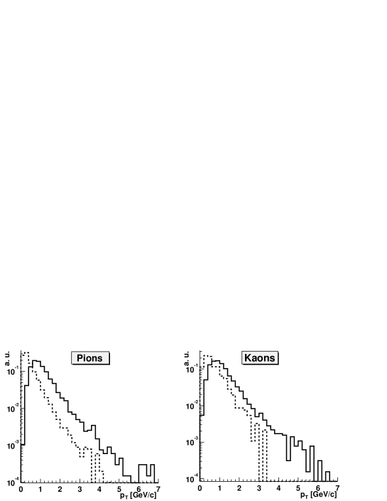
Figure 3.1: Distribution of charm meson decay products into pions and kaons. The solid lines represent the signal while the dashed line is the background [51].

For example, if the $<p_{t}>$ of the D⁰ is 1 GeV/c, the relevant decay channels, $K\pi\pi$ (for charged D), and $K\pi^{0}$ (for D⁰), have a majority of their tracks above 0.8 GeV/c. Similarly, if the $<p_{t}>$ of the underlying “soft” event is 0.4 GeV/c, the fraction of tracks with $p_{t}>$ 0.7 GeV/c is about 15% of the total. Reconstructing all tracks in the TPC online (with an emphasis on a high efficiency at high $p_{t}$), and keeping only the raw data along regions revealing high $p_{t}$ trajectories, can reduce the data volume by a factor of 5-6. Applying additional kinematical selection and secondary vertex topology criteria would further improve the selection of possible $D^{0}$ events. Simulations show that signal–to–event of 0.0013 and a background–to–event of 0.0116 [53] should be obtainable in ALICE. HLT can potentially reduce the data rate needed for the open charm program by a factor 5-10, thus increasing statistics and at the same time release DAQ bandwidth.

Di-electron trigger

The muon arm measures the $J/\psi$ and $\Upsilon$ spectra via the di-muon channel. A complementary study of these particles will be performed by reconstructing their leptonic decay into $e^{+}e^{-}$ and tracking these di-electrons through the TPC, TRD and ITS. The TRD will trigger on high $p_{t}$ tracks by online reconstruction of particle trajectories in the TRD chambers, and on the electron candidates by measuring of the total energy loss and the depth profile of the deposited energy. The true quarkonium trigger rate however is small (e.g. signal rate of $\Upsilon$ is $\approx$10^-2 Hz) and the trigger is dominated by the background. Depending on the set of cuts being used, a trigger rate of di-electron pairs of 300-700 Hz at dN_ch/dy=8000 is expected [36]. The main contributions to the background comes from:

• Electron pairs from Dalitz decays of $\pi^{0}$, $\eta$, $\rho$, $\omega$, $\phi$ and semi-leptonic decays of $B$ and $D$ mesons.

• Electrons or positrons from gamma conversions, Bremsstrahlung, and secondary interactions.

• Pions misidentified as electrons.

• Fake tracks from combinations of clusters from different tracks.

The HLT can be used to reject background events by two methods:

• Combining TRD tracklets with TPC and ITS tracking. The combined track fit allows for a more accurate determination of the momentum than by the TRD alone, and thus HLT will reject secondary electrons by sharpening the momentum cut.

• Utilizing dE/dx in the TPC. By identifying the particles using dE/dx information from the TPC, the background from misidentified pions can be reduced.

Simulations indicates that event rate reduction by a factor of ten can be achieved.

Di-muon trigger

The forward muon arm is designed to detect vector resonances via the $\mu^{+}\mu^{-}$ decay channel, and will run at the highest possible rate in order to record all muons with the lowest possible dead-time. The task of the di-muon trigger system is to select events containing the di-muon pair from the decay of $J/\psi$ and $\Upsilon$, where the background is mainly coming from the muons due to $\pi K$ decays.

The first level of the di-muon trigger consists of a transverse momentum selection based on the information from two dedicated trigger chambers. The trigger is optimized for two different $p_{t}$ thresholds in order to select low ($>$1 GeV/c) and high ($>$2 GeV/c) $p_{t}$ muons from the $J/\psi$ and $\Upsilon$ resonances, respectively. However, the coarse-grained segmentation of these trigger chambers does not allow a sharp $p_{t}$-cut, resulting in a rather large background trigger rate. The $p_{t}$ resolution can be improved by performing an additional tracking step within HLT using information from the muon tracking chambers, and thus achieve higher trigger selectivity, Table 3.1.

	L0	HLT
Low pt cut	2000 Hz	500 Hz
High pt cut	550 Hz	Few Hz

Table 3.1: Expected trigger rates of the di-muon detector [54]. The two $p_{t}$ -cuts correspond to the selection of $J/\psi$ and $\Upsilon$ resonances, respectively.

The expected background rejection factor by inclusion of HLT algorithm is 5-100.

Pileup removal in pp

In the case of p–p running, the foreseen running luminosity of 2$\times$10³⁰ cm^-2 s^-1 will result in an interaction rate of about 200 kHz. During the TPC drift time of about 90 $\mu$s, around 25 superimposed events will be captured in the TPC frame, leading to about 95% overhead in the data stream. These additional piled-up events will be displaced along the beam axis, and will not be used during offline analysis. Using HLT to reconstruct all tracks online, the tracks corresponding to the original triggered event can be identified while the tracks belonging to the pile-up events can be disregarded from the readout data stream. Simulations indicate that an overall event size reduction of $\sim$3/25 can be achieved while retaining an efficiency of more than 95% for the primary tracks of the event.

3.2.2 Data compression mode

The option to compress the data online provides a method that can improve the physics capabilities of the experiment in terms of statistics, even without performing selective readout. If the compression factor is high enough ($\geq$10), the full event rate can in principle be written to mass storage. Any data compression has to be performed with caution to assure the validity of the measured physical observables.

The TPC detector produces by far the largest amount of data in terms of event sizes, and any data compression scheme should therefore be optimized to efficiently and reliably compress the TPC data. TPC data are first compressed in the the TPC front-end electronics by the zero suppression, Section 2.4.3. Here, pedestal subtraction (setting threshold on the ADC values) and identification of the sequences in time direction is performed. The zeros between these sequences are then compressed by Run-Length Encoding (RLE), which means that the distance between the sequences are stored rather than storing the zeros themselves.

The data may be further compressed by applying standard data compression techniques such as entropy coding. These algorithms may be directly applied on the RLE ADC-data and allow bit-by-bit reconstruction of the original data set. Since these techniques normally use some form of coding table, they are not very computationally demanding, and can even be performed on dedicated hardware such as Field Programmable Gate Arrays (FPGA). Extensive studies of TPC data in the NA49 experiment, and simulated TPC data for ALICE, show that compression factors of  2 can be achieved using these techniques [55]. The most efficient data compression, however, is obtained by using compression algorithms which are highly adapted to the underlying TPC data. Such methods exploit the fact that the relevant information is contained in the reconstructed cluster centroids and the track charge depositions. These parameters can be stored as deviations from a model, and if the model is well adapted to the data the resulting bit-rate needed to store the data will be small. Since the clusters in the TPC critically depends on the track parameters, the reconstructed tracks and clusters can be used to build such efficient data models. In contrast to the entropy coding algorithms, such techniques do not keep the original data unmodified as the clusters are coded rather than the ADC data. However, from a data analysis point of view, only the effects on the physics observables are of importance. Studies carried out in this work indicate that compression factors of 6-10 may be achieved using such a compression scheme. The different available TPC data compression schemes and their performance are discussed in detail in Chapter 5.

3.3 Architecture

The HLT system will have to process an expected data rate of 10-20 GB/s. Given this large amount of data, and the complexity of the processing task, a massive parallel computing system is required. The HLT system is therefore planned to consist of a large PC cluster farm with several hundred up to a thousand separate nodes. The architecture of such a system is mainly driven by two constraints. Firstly, the data has an inherent granularity and parallelism defined by the readout segmentation of the detectors. Secondly, HLT is (in trigger mode) responsible for issuing a trigger decision based on information derived from a partial or complete event reconstruction. This means that the reconstructed data finally has to be collected at a global layer in which the trigger algorithms are implemented. Both of these requirements demand a hierarchical tree-like topology with a high degree of connectivity.

Figure 3.2: Data flow architecture of the HLT system [51]. The detector raw data is duplicated and simultaneously received by DAQ and HLT. The architecture follows a hierarchical structure, adapted to the parallelism of the data and the various tasks of the pattern recognition.

In parallel to the DAQ system (Section 2.5.3), the data is received from the front-end electronics via the DDLs into the receiving nodes of the HLT system, Figure 3.2. These processors constitute the first layer of the HLT system, and are referred to as the Front-End Processors (FEP). Each DDL is mounted on a HLT Readout Receiver Card (HLT–RORC) which is a custom designed PCI card hosted by every FEP. Several HLT–RORCs may be placed in each FEP, depending on the bandwidth and processing requirements. Every HLT–RORC will be equipped with additional co-processor functionality for designated pre-processing steps of the data in order to take load off the CPUs of the FEPs. The total number of HLT–RORCs is defined by the readout granularity of the detectors. For the TPC detector, which is the biggest contributor, the readout is divided into its respective 36 azimuthal sectors, where each sector is divided into 6 sub-sectors. Every sub-sector is read out by one DDL, and thus there will be 36$\times$6 = 216 DDLs for the TPC alone. Taking all detectors into account there will be a total of about 400 DDLs.

Data-flow

All detectors will ship their data upon a receipt of a L2–accept trigger distributed by the central trigger processor (Section 2.5.2). Before that time, the data remains within the domain of the front-end electronics. Table 3.2 gives an overview of the various detector links and their expected data payload.

		Sub-event size per DDL
Detector	Number of	Pb–Pb central	Pb–Pb per.
	DDLs	(kB)	(kB)
TPC	216	352	90
TRD	18	39	10
DiMuon	10	15
ITS	56	35

Table 3.2: Number of HLT detector links per detector and their data payload [51].

The associated L2–accept trigger rates for the TPC are limited to 200 Hz for Pb–Pb running and 1 kHz for p–p (Section 2.5.1). The other detectors can be triggered with 1 kHz, when triggered without TPC coincidence. This overview shows that the aggregate HLT input raw data stream amounts to a maximum of about 20 GB/s. The processing rates will vary as a function of trigger type and running scenarios. For instance in central Pb–Pb collisions the TPC trigger rate will be limited to 200 Hz due to pile-up protection, while for p–p collisions the TPC trigger rate may be as high as 1 kHz. The maximum HLT output data rate, however, is limited to the maximum taping rate of 1.25 GB/s. Consequently, both the maximum HLT input and output rates are defined almost independent of its detailed architecture and requirements.

The detailed data-flow within the HLT system will be defined according to the physics requirements and operating scenarios. However, the general structure depends to a large degree on the input and output data flow as stated above, Figure 3.2. The data is received on the HLT–RORC where the first part of the processing will take place using a Field Programmable Gate Array (FPGA) co-processor. In the case of the TPC this processing consists of local pattern recognition tasks, i.e. cluster finding and/or the Hough Transform. The data is then transferred into the main memory of the FEP over the PCI bus, where further processing can be made. After this the data is shipped to a node at the next level, which consists of as many nodes that are necessary to perform the processing needed. Here, the processing typically includes track finding within the TPC sectors. The output data produced by each level is again shipped to the next level of nodes until the final stage has been reached. In this way, the processing hierarchy follows a tree-like structure, where successive larger parts of an event are processed and merged as one comes closer to the root of the tree. At this global level all the necessary data has been collected into the final reconstructed event, i.e. tracks from the different sub-sectors are merged and fitted, and a final trigger decision for the event can be taken based on selection algorithms. The decision and the corresponding data is then passed to the DAQ system for readout and storage. The interface between DAQ and and HLT will consist of a number of DDL links between a set of HLT event merger nodes and a number of DAQ LDCs. The various processing tasks involved in the different levels are described in Chapter 4.

Hardware components

The HLT system will consist of a large scale generic computation farm, with standard PCs connected with a high bandwidth and low latency network. Given the huge commercial development within this field, the project has decided to keep custom hardware development at a minimum. This will thus enable the system to be very flexible with respect to selecting the type of processing node and network technology, and also delay this decision as much as possible due to the continuously drop in prices.

The design of the data flow, and exact processing sequence, determines much of the architecture and network topology which will be used. It has also impact on the requirements on the communication between each pair of the HLT nodes. Candidates for the network technology to be used are not yet fixed, but for the required bandwidth at least Gigabit Ethernet or a System Area Network (SAN) dedicated to communication in cluster solutions, is necessary. Possible choices which are considered are among others ATOLL, SCI and Myrinet.

The HLT–RORC will implement co-processor functionality by usage of Field Programmable Gate Array (FPGA). The FPGA basically implements a large array of freely programmable logic gates which can be connected in an arbitrary fashion. The relatively low clock rate of less than 100 MHz is compensated for by a very high degree of inherent parallelism. This makes the FPGA ideal for implementation of algorithm which can be executed in a highly parallel fashion, such as TPC cluster finding and the Hough Transform, Chapter 4.

Communication framework

An essential part of the HLT system is interprocess communication and data transport within the system. For this purpose a generic communication framework has been developed [56]. The framework has been designed with an emphasis on three main issues:

• Efficiency.

• Flexibility.

• Fault tolerance.

Efficiency in this context is primarily the minimization of CPU cycles used for transporting data, in order to keep as much CPU power as possible available for processing the data. The requirement for flexibility is a natural consequence from the fact that neither the topology nor the network interface is defined, and will be postponed as much as possible. Fault tolerance means that the framework has to be able to handle and recover from errors as autonomously as possible, and thus should not contain any single points of failure in which a fault can disable the whole system.

The framework implements an interface between different readout steps, by defining data producers – Publisher – and data consumers – Subscriber. In order to be as efficient as possible the data is not communicated between the different processes, but rather a descriptor of the data including a reference to the actual data in shared memory is sent. In this way data is stored in memory as long as possible, avoiding unnecessary copying of the data. The framework basically consists of a number of independent software components that can be connected together in an arbitrary fashion. The generic interface allows the processing modules to have a common interface which is independent of the underlying network interface.

Chapter 4 Fast Pattern Recognition in the ALICE TPC

The main processing task of the High Level Trigger system is online event reconstruction. Both event selection and efficient data compression needs a preceding pattern recognition step. The algorithms which have been developed for online reconstruction of the TPC data, together with a performance evaluation, are presented in this chapter.

4.1 Track reconstruction methods

Every charged particle traversing the detectors leaves a number of discrete hits that allow spatial allocation of the particle trajectory. The task of the reconstruction algorithms is to assign these space points to tracks and to reconstruct the particle kinematics. Reconstructing a particle is equivalent to finding the parameters that uniquely define its path in space. From the reconstructed parameters one can find the physical properties of the particles that passed through the detector.

In general, track reconstruction is a two-folded problem:

• Track finding.
  The input to the track finder is a list of all hits in selected regions or the complete detector. The task is to decide which hits are made by a specific particle, and group these hits into a number of subsets. All the hits within a subset belong to the same particle trajectory, and the number of subsets corresponds to the number of particles traversing the detector.

• Track fitting.
  The task of the track fitting procedure is to estimate the parameters of the curve describing the trajectory. The input is thus the positions of all the hits in a subset provided by the track finder, whereas the output is a list of particles represented by an estimate of the track parameters.

Traditionally these two steps are performed separately, but certain applications also combine them.

The increasing complexity in terms of track densities and data sizes in the LHC experiments, poses high demands on the track reconstruction algorithms. Both real-time applications and offline analysis require fast and robust methods in order to efficiently process the large amount of data produced. A great variety of pattern recognition methods exist within the field of high-energy physics, each with their advantages and disadvantages with respect to complexity and performance. In the following a brief overview of the main track finding and fitting methods is given.

Local track follower

The principle of a track follower is to assign hits to the track candidate under construction based on the local information of the track. The track candidate is typically initiated by building short track segments including only a few hits. These track segments are subsequently extrapolated between the adjacent active detector layers. For every step, the algorithm tries to assign a new hit to the track, and the choice is being made by applying $\chi^{2}$ criteria of a temporary track fit. Once a new hit has been assigned, the track parameters are updated and the search is continued.

The advantage with the local track follower approach is its simplicity with respect to both data access (since it only needs to access a limited number of hits at the same time) and the selection criteria for each step. This makes this method efficient when the hit and track densities are relatively low. However, when the hit density becomes high, such an algorithm might get confused on the basis of simple $\chi^{2}$ criteria. This will lead to tracks being split or spliced together in unpredictable ways, and thus effect the track finding efficiency.

Track-Road methods

The Track-Road methods are similar to the local track follower algorithms. However, Track-Road methods build tracks by interpolating within possible trajectory roads in the detector. This is done by choosing hits in the outermost and innermost layers of the detector, and interpolate between combination of these hits to obtain the complete tracks. Because of the combinatorial nature of these methods, they are more computationally demanding than the local track follower algorithms.

Template matching methods

Many of the ambiguities at track crossings in detector layers that arise from local extrapolation algorithms can be overcome with global information of the complete trajectory. The global information can be obtained by using different template matching methods. Here, a list of predefined trajectories, called templates, are computed based on the equations of particle motion. The templates are then overlaid on the data from the detector, and a set of conditions is applied to determine whether a match exists. Originally, the templates were static, and the resolution of the track parameters were defined by the number and granularity of the template set being used. In order to overcome these shortcomings, different adaptive approaches have been developed.

The Elastic Tracking [57, 58] is an approach that defines the templates in a dynamical way, by allowing the predefined trajectories to deform via a set of mathematical equations to match a pattern in the data. This approach has proved to be very efficient in high track density environments [59]. It also offers the possibility to do tracking on raw detector data without any data pre-processing. However, the high efficiency comes at the expense of very high processing time and memory requirements.

Hough Transform (Histogram method)

Histogram methods are closely related to template matching methods. They transform particle hits which makes up a pattern into a suitable parameter space for further evaluation. Most common is the Hough Transform, which was initially proposed to detect particle tracks in bubble chamber pictures [60]. A hit or a subset of hits on a particle trajectory is transformed into curves in a $n$-dimensional histogram, in which the hits give a “vote” to all the possible trajectories they can possibly belong to. Once all the hits on a trajectory have been transformed, the intersection of these curves will correspond to the parameters of the track. In this way the problem of recognizing global patterns is reduced to the problem of local peak detection in parameter space.

The advantages of the Hough Transform is its noise robustness and its simplicity with respect to hardware implementation. However, the transformation is also very computationally demanding, in particular with respect to the memory requirements.

Kalman filtering

The Kalman filter method is a method for track finding and fitting which is very commonly used in high-energy physics experiments [61, 62, 63]. In the framework of the Kalman filter, the change of the parameters of a track along its path is regarded as the dynamical evolution of a stochastic state vector. The algorithm basically consists of a succession of alternating prediction and filter steps. In the prediction step the current state vector is extrapolated to the next detector layer, taking into account multiple scattering, energy loss and Bremsstrahlung in the case of electrons. In the filter step the next hit on the trajectory is selected based on the predictions of the state vector, and the state vector is updated accordingly.

The main advantage of the Kalman filter is that is a method for simultaneous track recognition and track fitting. It also provides a natural way of extrapolating the tracks between different detectors. On the other hand, the Kalman filter needs an initial set of “seeds” which has to be provided by a preceding pattern recognition step.

Neural Networks

The application of neural network methods is known to offer good approximate solutions to different optimization problems, among them track finding problems in high-energy physics [64]. The basic idea is to set up an energy function whose minimum corresponds to the solution of the pattern recognition problem. The dynamical evolution of the network should then always decrease the energy and rapidly converge to a solution. This method has proven to give comparable results with other track finding approaches [65], and is generally less time consuming. One major drawback, however, is absence of a track model in the formalism, and the fact that it has to be supplemented with a separate track fitting procedure.

Track reconstruction in the TPC

In case of the TPC, the signals produced by the traversing particles correspond to two-dimensional charge distributions, called clusters, Section 2.4.1. The centroid of these distributions corresponds to the three-dimensional space points along the particle trajectories. Pattern recognition in the TPC is often classified in two main categories; an sequential and iterative approach.

Sequential pattern recognition

In the sequential case the pattern recognition is performed in two sequential steps. In the first step, the cluster centroids are calculated. A cluster finder searches the raw ADC data for local maxima in the two dimensional charge distributions. If an isolated cluster is found, the centroid position in pad and time is calculated. In the case of overlapping clusters, the charge distributions have to be separated by unfolding procedures. However, due to the missing information about the track parameters of the crossing tracks, neither the shape nor the size of the clusters are known at this stage. Furthermore, the number of tracks contributing to the distribution are unknown. Therefore, the distributions cannot easily be unfolded, and the resulting centroids are error-prone and may result in a loss of tracking performance. Together with the position of the pad-row plane, the centroids provide the three dimensional coordinates which are interpreted as the particle crossing point with the pad-row plane. In the second step, the list of space points serve as an input for the track finder which connects the space points into track segments. The track finding problem is typically solved by a local track follower or a Kalman filter approach.

This method is the conventional approach for track reconstruction and has been successfully been used with TPCs in a relatively low occupancy environment. Examples are the reconstruction programs for the NA49 [47] and the STAR [48] experiment. In the ALICE experiment however, the detector occupancy in the TPC may well reach values of up to 50% (Figure 4.1). In such a scenario the amount of overlapping clusters will be very high, and it is generally expected that the performance of a simple cluster finder will be low. A cluster model for the overlapping charge distributions is likely to improve the results.

Iterative pattern recognition

In the iterative track finding approach, the procedures of cluster finding and track finding are not separated into two sequential steps, but rather done in a more parallel or iterative fashion. In this case parts of the track finding is solved prior to the cluster finding. In a first step “track seeds” are found for instance by using a combinatorial approach based on cluster centroids located at larger radius (where the occupancy is low) or by applying track finding algorithms like the Hough Transform directly on the raw ADC data. Based on the list of found track segments, one returns to the raw-data and reconstruct the clusters along the trajectories. Since the cluster model is a function of the crossing tracks and detector specific parameters and the electronics, the track model provides an estimate of shape and size of the clusters. Hence the charge distributions can be fitted to a known shape. Based on the additional knowledge of the tracks passing nearby and therefore possibly contributing charge to the clusters, overlapping clusters can be properly deconvoluted. This approach was used in the NA49 [47].

4.2 The ALICE tracking environment

The experimental setup of the ALICE experiment consists of the central barrel placed inside the L3 magnet and the forward detectors (Section 2.3). The main tracking detector is the TPC detector, which has a coverage of $|\eta|<$ 0.9 and full azimuth.

4.2.1 Particle multiplicity and detector occupancy

The ALICE experiment is designed to handle a charged particle multiplicity corresponding to 8000 charged particles per unit rapidity, dN_ch/dy=8000 [32]. This estimate is regarded as an extreme assumption, and is based on a comparison between different event generators for Pb-Pb collisions at the LHC energy of $\sqrt{s_{NN}}$=5.5 TeV. The predicted charged particle multiplicity at the mid-rapidity, however, varies strongly, ranging from dN_ch/dy of about 1500 to 7-8000, depending on the generator used.

In order to study detector performance, it is more convenient to use pseudo-rapidity, $\eta$, instead of rapidity since the pseudo-rapidity is a geometrical unit while the rapidity depends on particle composition and $p_{t}$-spectra. It should however be noted that the multiplicity per unit rapidity is 10-20% more at mid-rapidity than the multiplicity expressed in units of pseudo-rapidity [31]. This means that a charged particle density of dN_ch/d$\eta$=8000 is 10-20% higher than the extreme assumption of dN_ch/dy=8000.

The ALICE Technical Proposal was written when the highest available nucleon-nucleon center of mass energy results was $\sqrt{s_{NN}}$=20 GeV (CERN SPS), i.e. a factor of 300 less than the LHC energy. Since that time, new data from RHIC at energy up to $\sqrt{s_{NN}}$=200 GeV has become available, and the event generators have been correspondingly updated. In Table 4.1 the results from the most common generators, HIJING (Heavy-Ion Jet INteraction Generator), DPMJET (Dual Parton Model) and the SFM (String Fusion Model) are summarized.

Generator	Comments	dNch/d$\eta$ at $\eta$=0 (approx.)
HIJING 1.36	with quenching	6200
	without quenching	2900
DPMJET-II.5	with baryon stopping	2300
	without baryon stopping	2000
SFM	with fusion	2700
	without fusion	3100

Table 4.1: Charged particle multiplicity simulated by different event generators [31].

A detailed description of the processes included and parameters used for each of these event generators can be found in [31] and references therein. Results show that large differences for dN_ch/d$\eta$ still exists, and even in the framework of a single generator the density is strongly model dependent. Furthermore, none of the current generators reproduce the multiplicities obtained from the theoretical extrapolations from RHIC described in Section 1.4 on page 1.4, which indicates values of about 2000-3000. Because of the large uncertainty in the particle multiplicity and the fact that extrapolation from RHIC results are still quite large ($\sim$30), the value of up to 8000 is still being considered as the design value by the collaboration in order to provide a absolute safety margin with respect to detector and software design. From a pattern recognition point of view, tracking algorithms should be developed that are capable of handling all possible scenarios.

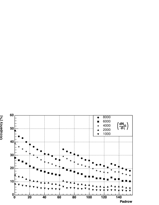
Figure 4.1: Simulated occupancy in the TPC as a function of pad-row number. The occupancy is calculated as the ratio between signals above threshold and the total number of digits. The steps are due to change in pad-sizes (Table 2.1).

In Figure 4.1 the simulated detector occupancy for the TPC is shown as a function of radius (represented by the pad-row number) for different multiplicities. For dN_ch/d$\eta$=8000 it reaches $\sim$50% for the innermost padrows, and drops to less 20% for the outermost.

4.2.2 Magnetic field settings

The central detectors are placed inside the L3 magnet which provides a solenoidal magnetic field. In general, the field strength selection in a heavy ion experiment is a compromise between low momentum acceptance, momentum resolution and tracking and trigger efficiency. In the ALICE experiment, the desired low momentum cut-off is determined by the ability to probe the soft hadronic regime, i.e. collective effects, detection of decay products of low $p_{t}$ hyperons, and identical particle interferometry. In the high momentum regime, the resolution has to be sufficient to measure the leading particles of high energy jets, and to measure the decay products of heavy quarkonium. The ideal field strength for hadronic physics, maximizing the reconstruction efficiency, is around 0.2 T, while for the high $p_{t}$ observables the maximum field strength the L3 magnet is able to produce, 0.4-0.5 T will most likely be the best choice [31]. Since the high $p_{t}$ observables are the ones which are limited by statistics, ALICE will run mostly at the higher magnetic field setting.

4.2.3 Particle trajectory in a magnetic field

A charged particle moving in a homogeneous magnetic field follows a circular motion in the plane perpendicular to the field. This is commonly referred to as the bending plane of the track. The momentum component along the magnetic field is left unchanged. These two components thus form a helix path in space. A description of the track model and helix parameterization can be found in Appendix A. The assumption that a particle follows a helical trajectory is exact when the magnetic field is constant and one neglects energy loss and multiple scattering. For a particle with unit charge, the relation between the magnetic field $B$ [T], and the curvature of the track, $\kappa$ [m^-1] is given by

$$p_{t}=\frac{0.3B}{|\kappa|}\hskip 28.45274pt[\mathrm{GeV}]$$ (4.1)

Once the $p_{t}$ of the particle has been determined, the remaining components of the particle momentum can be calculated from

$$p_{z}=p_{t}\tan\lambda$$

$$p=\sqrt{p_{t}^{2}+p_{z}^{2}}$$ (4.2)

where $\lambda$ is the dip-angle of the track.

The curvature and the dip-angle of a track segment is determined by fitting the individual space points along the trajectory. The accuracy of which the curvature and thus the momentum can be measured is limited by the space point errors. The relation between the azimuthal position resolution of a single space point and the relative transverse momentum error can be parameterized by [66]

$$\frac{\Delta p_{t}}{p_{t}}=\frac{\sigma_{r\phi}p_{t}}{0.3BL^{2}}\sqrt{\frac{720}{N+4}}$$ (4.3)

where $L$ is the total visible track length, $N$ is the number of measured space points on the track and $\sigma_{r\phi}$ is the error of the position measurement. For the ALICE TPC $L$ and $B$ are given by the overall design parameters of the detector, while $N$ and the space point resolution are defined by the design of the readout chambers (Section 2.4.2).

In addition to the track measurement errors, the obtained momentum resolution will be limited by multiple scattering and energy loss. These effects cause the particle trajectory to deviate from a helix. Furthermore, the resolution will also be limited by detector readout specific effects such as diffusion and angular effects etc. (Section 2.4.1, page 2.4.1), and the noise imposed by the electronic readout chain.

4.3 The AliROOT framework

The complete ALICE detector setup is described and simulated within the AliROOT framework [67], which is based on the ROOT software package [68]. The framework consists of a set of software tools which mimic the different steps of data processing required in the ALICE experiment. An overview of the functionality of the framework is shown schematically in Figure 4.2.

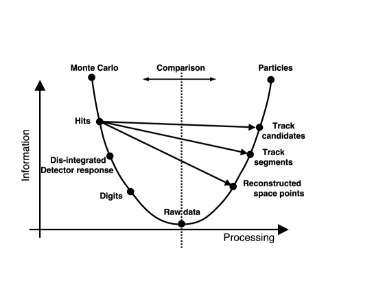
Figure 4.2: Functionality overview of the AliROOT framework [31].

Data are generated via simulation programs, i.e. event generators and detector response simulations, and are then transformed into the data format produced by the detector. The data produced by the event generators contain the full information about the generated particles, i.e. particle type and kinematics. These data then serve as input to the detector simulation chain, in which the information is disintegrated to that generated by particles when traversing the detector. The outcome of the detector simulation is representative of real data measured in a real detector. This data can thus be used as input for the various reconstruction and analysis chains, which can be evaluated by comparing the final reconstructed particles with the generated ones. Each detector is described as an independent module that contains the code for both simulation and reconstruction.

4.3.1 Event simulation

The theoretical uncertainty with respect to the outcome of heavy ion collisions at LHC makes it necessary to use and compare several models for the simulation of the final state particles in an event. Consequently, a variety of different event generators have been implemented within the AliROOT framework. In order to evaluate the reconstruction and analysis algorithms in AliROOT, a generator capable of simulating a typical “background” event for various multiplicities is needed. For this purpose a parameterization of the HIJING generator, which is based on parameterized $\eta$-density and $p_{t}$ distributions of charged and neutral pions and kaons was encoded. In this model, the $\eta$-distributions have been obtained from a HIJING simulation of central Pb-Pb collisions, and the $p_{t}$ distributions of the pions are based on $p_{t}$ measurements at $\sqrt{s}$=1.8 TeV [69]. The corresponding kaon $p_{t}$ distribution is obtained from the pion distribution by m_t scaling. To simulate a multiplicity of e.g. dN_ch/d$\eta$ = 8000, the $\eta$-distribution is scaled in such a way that 8000 charged particles per event are produced within the range $|\eta|<$0.5. Lower multiplicity events are scaled similarly. All the sample events used in this work have been produced using this parameterization.

4.3.2 Simulation of detector response

Once the collision is simulated by an event generator, the final state particles are fed to a particle transport program. For simulating particle transport in AliROOT the GEANT3 package is currently being used. The particles are transported in the material of the detector, simulating the interaction and the energy deposition that generates the detector response. From the energy deposition, the “ideal” detector response resulting from the traversing particles is generated. This response is subsequently digitized and formatted according to the output of the detector front-end electronics. Thus, the final results are expected to closely resemble the real data produced by the ALICE detector system.

In the special case of the ALICE TPC detector, a dedicated microscopic simulator has been implemented in AliROOT [70]. All major physical processes are incorporated in this simulator, including parameterization of the ionization in the gas, generation of secondary electrons, diffusion of electrons, electron attachment, E$\times$B effect near the anode wires, and a complete pad and time response determined by the readout-chamber geometry and electronics parameters.

Simulation of the physical processes in the TPC

The ionization in the gas is basically described by the generation of primary and secondary electrons. The electromagnetic interactions of the initial particle with the TPC gas lead to the release of the primary electrons. If these electrons have sufficient kinetic energy they will further ionize the gas and produce secondary electrons, creating the electron cluster. The mean distance, $D$, between two primary ionization’s can be expressed as

$$D=\frac{1}{N_{\mathrm{prim}}\cdot f(\beta\gamma)}.$$ (4.4)

Here $N_{\mathrm{prim}}$ is the number of primary electrons per cm produced by a minimum ionizing particle (MIP), and $f(\beta\lambda)$ is the Bethe-Bloch function. The energy loss function is parameterized from a fit to energy-loss data for 90% Ar, 10% CH₄. The energy loss released in the primary ionization to atomic electrons has, if one neglects the atomic shell structure, a close to 1/E² dependence. For light gases the distribution has a slightly steeper dependence, and in the simulation a 1/E^2.2 parameterization is used.

The total number of secondary electrons, N_tot, created in a cluster is given by,

$$N_{\mathrm{tot}}=\frac{E_{\mathrm{tot}}-I_{\mathrm{pot}}}{W_{i}}+1,$$ (4.5)

where $E_{\mathrm{tot}}$ is the energy loss in a given collision, $W_{i}$ is the effective energy required to produce an electron-ion pair and $I_{\mathrm{pot}}$ is the first ionization potential. The simulated clusters are initially point-like objects, and no distinction between primary and secondary electrons are done.

The produced electrons drift through the gas with an constant effective drift velocity. During the drift, the electron cloud is subject to diffusion, which is described by a three-dimensional Gaussian distribution,

$$P(x,y,z)=\frac{1}{\sqrt{2\pi\delta_{T}}}\exp\left[-\frac{(x-x_{0})^{2}}{2\delta^{2}_{T}}\right]\cdot\frac{1}{\sqrt{2\pi\delta_{T}}}\exp\left[-\frac{(y-y_{0})^{2}}{2\delta^{2}_{T}}\right]\cdot\frac{1}{\sqrt{2\pi\delta_{L}}}\exp\left[-\frac{(z-z_{0})^{2}}{2\delta^{2}_{L}}\right],$$ (4.6)

where $(x_{0},y_{0},z_{0})$ is the electron creation point, and the transversal, $\delta_{T}$, and longitudinal, $\delta_{L}$, diffusion are given by the drift length, $L_{\mathrm{drift}}$, and gas coefficients, $D_{T}$ and $D_{L}$

$$\delta_{T} = D_{T}\sqrt{L_{\mathrm{drift}}}$$

$$\delta_{L} = D_{L}\sqrt{L_{\mathrm{drift}}}$$ (4.7)

During the drift through the gas the electrons can be absorbed in the gas by the formation of negative ions. This process has been simulated by assuming a probability of electron capture of 1% per m drift per ppm of O₂.

Near the anode wires, the magnetic field and electric fields are no longer parallel, and because of the Lorentz force the electrons experience a displacement along the wire direction. If an electron enters the readout chamber at point $(x_{0},y_{0})$, it is displaced in the $x$-direction (assuming that the wires are placed along the $x$-axis). The new position of the electron is given by,

$$x=x_{0}+\omega\tau(y-y_{0}),$$ (4.8)

where $y$ is the coordinate of the wire on which an electron is collected, and $\omega\tau$ is the tangent of the Lorentz angle.

Simulation of the signal generation

When the electron cluster enters the readout chambers, the electrons are accelerated in an increasing electric field towards the anode wires. Once the electric field is strong enough, an avalanche is created. The amplitude of this avalanche is determined by the high voltage applied to the wire, and is subject to fluctuations. The resulting number of electrons created can be described by an exponential probability distribution function,

$$P(q)=\frac{1}{\bar{q}}\cdot\exp\left(-\frac{q}{\bar{q}}\right),$$ (4.9)

where $\bar{q}$ is the mean avalanche amplitude.

An electron which is collected on the anode wire leaves an ion behind which induces a charge on the pad plane. This charge is integrated over the pad area, and the induced charge distribution in the pad plane is determined by the Pad Response Function (PRF). In the simulation, a two-dimensional PRF is computed for the pad-geometries planned for the ALICE TPC. This calculation also incorporates possible signal measurements from the neighboring wires (“crosstalk”). The time signal is obtained by convolving the avalanche with the shaping function of the preamplifier/shaper, and sampled at a given frequency. The generated signal is then superimposed with a random electronic noise. This noise is described by a Gaussian with RMS equal to 1000 $e$. The simulated signal is finally digitized using the predefined dynamic range of the electronics and by applying zero suppression.

4.3.3 The Offline reconstruction chain

The ALICE Offline reconstruction algorithm is based on the Kalman filtering approach [63]. The reconstruction chain starts with a cluster finder in the TPC, which provides the space points that are used for tracking with the Kalman filter. The overall tracking then starts with track seeding in the outermost pad-rows of the TPC. It begins with a search for all pairs of points which are projecting to the primary vertex. Different combinations of the pad-rows are used with and without a primary vertex constraint, in order to obtain both primary and secondary tracks. When a reasonable pair of points is found, parameters of a helix going through these points and the vertex are calculated. These parameters and the corresponding covariance matrix are then taken as the initial track candidate which are propagated from the outermost point to the inner point using the Kalman filter. If at least half of the possible points between the initial ones were successfully associated with the current track candidate, it is stored as a valid seed and the search continues. Each seed is then propagated through the entire TPC.

One of the main shortcomings using the Kalman filter in ALICE is that it depends on good seeds to start a stable filtering procedure. In the present approach this is very computationally demanding, as the search is done in a straightforward combinatorial way. Another drawback is that the clusters have to be reconstructed prior to the track finding, which is a difficult task in regions with high occupancy and cluster overlapping. However, recent developments deal with this problem utilizing an iterative tracking approach, i.e. by performing cluster finding in parallel to track finding [71]. In this way, information about the tracks which produce the clusters is available, and deconvolution is more easily performed.

4.4 Premises

The pattern recognition algorithms implemented in this work are primarily developed for the ALICE High Level Trigger system. In this context there are two main considerations:

• Computing requirements.

• Parallelization.

The computing requirements define the processing power in terms of processing time and memory requirements needed to reconstruct a complete event. From the High Level Trigger point of view, the time available for this task is constrained by the event rate. The amount of processing power needed for the full system will critically depend on the processing requirements for the individual processing modules. The algorithms should therefore be optimized with respect to both efficient data organization and the minimization of computing intensive tasks. The latter consideration is related to the fact that the readout of the detector is done in parallel, Section 3.3. This defines the first level of the HLT architecture, in which the first part of the pattern recognition is performed. Furthermore, merging the data from different parts of the detector implies copying data over network, and should therefore be avoided as far as possible. Effort has therefore been made to implement the processing schemes in a highly modular fashion, allowing for a high degree of parallelization.

As part of this work, two different TPC pattern recognition approaches were implemented and evaluated on simulated ALICE TPC data. They are in the following referred to as sequential tracking and iterative tracking, reflecting the two main TPC track reconstruction methods introduced on page 4.1.

4.5 Sequential tracking

The implemented sequential tracking scheme consists of 4 main successive processing modules, referred to as Cluster Finder, Track Finder, Track Fitter and Track Merger. The algorithms used for the Cluster Finder and the Track Finder are based on the reconstruction scheme implemented and used in the STAR L3 trigger [72]. All algorithms, and their implementation issues are described in the following.

4.5.1 The Cluster Finder

The cluster finder algorithm is an implementation of a straightforward sequence matching technique. The main emphasis of the algorithm is to optimize the program with respect to CPU time and memory access. A FPGA implementation of the algorithm has been implemented [73] for the purpose of utilizing the co-processor functionality planned for the Front-End Processors.

The basic functionality of the algorithm is to group sequences in the pad-row-plane which belong to the the same cluster and calculate the two-dimensional centroid, ($\lambda_{\mathrm{pad}},\lambda_{\mathrm{time}}$), by a weighted mean,

$$\lambda_{\mathrm{pad}}=\frac{\sum_{i}q_{i}p_{i}}{\sum_{i}q_{i}}\hskip 28.45274pt\lambda_{\mathrm{time}}=\frac{\sum_{i}q_{i}t_{i}}{\sum_{i}q_{i}}.$$ (4.10)

Here $q_{i}$ is the ADC-value of a given $(p_{i},t_{i})$ (pad,time) bin. A flow diagram of the algorithm is shown in Figure 4.3. The input to the cluster finder is a list of sequences for each pad. For every new sequence the centroid position in the time direction is calculated. This temporary mean is then compared to the sequences in the previous processed pads. During this step there are two possible outcomes:

• A match is found. This means that there is another sequence on the neighboring pad that overlaps with the current sequence. The two sequences are then merged and the mean in both pad and time are calculated.

• No match was found. In this case, the sequence is regarded as the start of a new cluster.

The essential feature of the algorithm is that it enables the program to handle all sequences in two distinct lists: The current pad list and the previous pad(s) list. This also allows the loop over the data only once, while performing all the calculations on-the-fly. Consequently, it is assumed that the input data stream is ordered in pad and time, i.e. all sequences on a single pad are received before the successive pad. Thus, the current pad list contains information about the sequences on the pad which are currently being processed, while the previous pad(s) list contains the clusters on the previous pad(s). A cluster is considered complete once there are no matching sequences on the current pad.

Figure 4.3: Flow diagram of the HLT Cluster Finder algorithm.

In the case of overlapping clusters, a simple cluster deconvolution scheme is applied. A check is performed on each sequence whether there exists a local minimum in the charge values. If such a minimum exists, the sequence is separated into two sequences by splitting at the time-bin containing the minimum charge. Following the same procedure in the pad direction, a check is done whether there is a local minimum in the pad charge for the cluster under construction. If this is the case, the matching cluster on the previous pad is not merged, but considered complete, while the sequence on the current pad is considered as a new cluster.

In addition to the cluster centroids, also the shape of the cluster is needed as additional information for the estimation of the space point errors, see next section. The shape can be represented by the widths of the cluster in the two dimensions, and is thus calculated as the RMS of the distributions.

In Table 4.2 the space point resolution obtained with the algorithm is listed for isolated clusters. The estimates are obtained by comparing the reconstructed centroids with pad-row plane crossings of the the simulated particle trajectories. The results are averaged over all primary tracks with $p_{t}$ $\geq$ 0.1 GeV which cross the entire TPC volume ($|\eta|<$ 0.9). The values correspond to the standard deviation obtained by performing a Gaussian fit of the distributions. For reason of comparison, also the results from the Offline cluster finder algorithm are shown. The resolutions are in the order of 0.8-1 mm and 1-1.4 mm for the pad and time direction, respectively. The results for the Offline cluster finder are slightly worse than the HLT cluster finder, which may be due to a wrong splitting of a few but large pathological clusters.

	Pad direction [mm]		Time direction [mm]
	HLT	Offline	HLT	Offline
Inner chambers	0.99	1.10	1.33	1.50
Outer chambers	0.88	0.96	1.14	1.23

Table 4.2: Space point resolution obtained using the HLT Cluster Finder on isolated clusters. For comparison, the results from the Offline cluster finder algorithm are also listed.

Space point errors

In addition to the three dimensional space point coordinates of the clusters, an estimate of the errors of the space points is needed for the track finding procedure. Similar to the cluster widths, the errors are determined by the diffusion and angular spread of the drifting electron cloud, and are thus dependent of detector specific parameters and the track parameters, Section 2.4.1. However, since the cluster finder does not have any information about the tracks, the errors are assumed to be proportional to the calculated RMS-values of the clusters. The coefficients have been found by comparing the reconstructed space points with the pad-row crossing points of the simulated tracks, and parameterizing the errors as a function of the cluster widths for both pad and time direction.

4.5.2 The Track Finder

The track finding algorithm is a local track follower algorithm. Its main feature is that it incorporates a transformation on the space points commonly referred to as conformal mapping. The purpose of this transform is to describe the circular motion of the particle trajectory in the bending plane by a linear parameterization. Since fitting straight lines is significantly less computationally demanding than fitting circles, the effect of the transform is to minimize the amount of calculations needed for the fitting procedures of the track finding algorithm.

Conformal mapping

The purpose of the conformal mapping is to transform the points on a circular pattern into a space where it can be described using a linear relation. Denoting the conformal space by ($x^{\prime},y^{\prime}$), a space point ($x,y$) transforms in according to,

$$x^{\prime} = \frac{x-x_{t}}{r^{2}}$$

$$y^{\prime} = -\frac{y-y_{t}}{r^{2}}$$

$$r^{2} = (x-x_{t})^{2}+(y-y_{t})^{2}$$ (4.11)

where the point (x_t,y_t) is a fixed point on the circle. In order to derive the linear relationship between points in conformal space, consider two points ($x,y$) and ($x_{t},y_{t}$) on a circle with center $(x_{c},y_{c})$ and radius $r_{c}$. For both points the following relations are then valid,

$$r_{c}^{2} = (x-x_{c})^{2}+(y-y_{c})^{2}$$

$$r_{c}^{2} = (x_{t}-x_{c})^{2}+(y_{t}-y_{c})^{2},$$

and therefore,

$$x^{2}+y^{2}=2x_{c}(x-x_{t})+2y_{c}(y-y_{t})+x_{t}^{2}+y_{t}^{2}.$$

Inserting the relations,

$$x^{2} = (x-x_{t})^{2}+2xx_{t}-x_{t}^{2}$$

$$y^{2} = (y-y_{t})^{2}+2yy_{t}-y_{t}^{2}$$

and the reverse transformation from Equation 4.11,

$$x = x^{\prime}r^{2}+x_{t}$$

$$y = -y^{\prime}r^{2}+y_{t}$$

results in,

$$(x-x_{t})^{2}+(y-y_{t})^{2}=2r^{2}[x^{\prime}(x_{c}-x_{t})-y^{\prime}(y_{0}-y_{t})],$$

and together with the definition of $r^{2}$ in Equation 4.11 this gives

$$y^{\prime}(x^{\prime})=\frac{x_{c}-x_{t}}{y_{c}-y_{t}}x^{\prime}-\frac{1}{2(y_{c}-y_{t})}=a_{y^{\prime}}x^{\prime}+b_{y^{\prime}}.$$ (4.12)

Equation 4.12 thus provides a linear parameterization of the circle in conformal space, Figure 4.4.

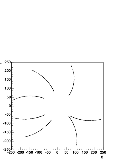
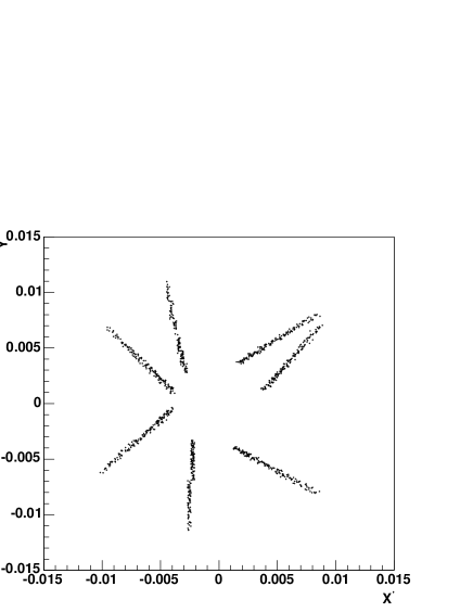
Figure 4.4: Conformal mapping of space points lying on the circular track segments. Each point in $xy$-space (left) is transformed into conformal space (right) using the vertex as a fixed point on the circle.

The transformation needs a fixed point, ($x_{t},y_{t}$), on the circle. In the case of track finding, this point can be replaced by the collision vertex coordinates if the track is assumed to originate from a primary particle. Alternatively, one can use the first point associated on the track. In that case, one assumes that the track originate from a secondary vertex.

The track follower

The track finding procedure is based on a follow-your-nose method initially proposed in [74]. The algorithm consists of building track segments by combining space points which are co-linear in the conformal space.

The first step of the algorithm consists of data organization. An essential part of the algorithm is to organize the space points in a efficient manner, so that the track finder has fast access to all the space points when building the track segments. This is done by assigning the space points to special sub-volumes in ($r,\phi,\eta$), where $r$, $\phi$ and $\eta$ correspond to pad-row number, polar angle and pseudo-rapidity, respectively. A sub-volume is denoted using the corresponding indexes ($i_{r},i_{\phi},i_{\eta}$). Every space point is uniquely associated with one sub-volume, and one sub-volume can of course contain many space points. The sub-volumes merely acts as containers for the space points, which in the implemented program correspond to a list of pointers to the respective space points structures in memory.

After transforming the space points into conformal space and organizing them into sub-volumes, the actual track finding starts. The tracks are being initiated by building track segments, and the search is starting at the outermost pad-rows. A space point is chosen as the starting point, $S$, in which the corresponding sub-volume is denoted ($i_{r}^{S},i_{\phi}^{S},i_{\eta}^{S}$). During the search, only space points which are in the nearby sub-volumes are considered. More specific, this corresponds to the sub-volumes satisfying the conditions:

$$i^{S}_{r}-N\leq j_{r}\leq i^{S}_{r}-1$$

$$i^{S}_{\phi}-1\leq j_{\phi}\leq i^{S}_{\phi}+1$$

$$i^{S}_{\eta}-1\leq j_{\eta}\leq i^{S}_{\eta}+1$$ (4.13)

where $N$ is a tunable parameter of the program. In this context, the distance, $d$, between two points is defined as

$$d=|i^{S}_{r}-i_{r}^{j}|\times(|\phi^{S}-\phi^{j}|+|\eta^{S}-\eta^{j}|).$$ (4.14)

The space points which are closest together are linked, and the search is continued until a certain number of space points is reached.

Once the track segments are obtained, the corresponding points are fitted to straight lines in conformal space and in the $(s,z)$ plane. The tracks are then build by associating new space points to the track which are close to the fit. The search continues from the outer pad-rows towards the inner pad-rows. When searching for a new space point, the nearby sub-volumes according to Equation 4.13 are being searched. For every step there are three possibilities:

• There are no points in the sub-volumes.
  If the track already has enough space points assigned, the track is considered a finished track, and the assigned points are removed from the available space point list. If the track does not have enough points assigned, the track is rejected and the space points are kept in the event.

• There is one space point in the sub-volumes.
  If the space point gives a updated track fit with acceptable $\chi^{2}$, the point is included and the track parameters are correspondingly updated. Otherwise the track is considered a final track if the number of already assigned space points is sufficient. Otherwise the track candidate is deleted and the space points made available for further tracking.

• There are several space points in the sub-volumes.
  In this case the program can either search through all the space point candidates and choose the one which gives the best $\chi^{2}$ of the track fit, or it can search through the list until a space point which gives good enough fit is found.

A flow diagram of the algorithm is illustrated in Figure 4.5.

Figure 4.5: Flow diagram of the Track Follower algorithm.

The performance of the algorithm on a given event sample is governed by the values set for the various tracking parameters. These typically include the granularity of the sub-volumes, maximum allowed $\chi^{2}$ during the track building and minimum number of hits on a valid track.

Non-vertex tracking

The Track Finder can perform two tracking passes, where the second pass takes the unused space points from the first pass as an input. In this case, the Track Finder does not apply any vertex constraint when building the tracks, and the conformal mapping is done relative to the first point associated with the track.

Due to the fact that most of the interesting tracks are in fact originating from the area of the main vertex, this option is in general not applied. Also, secondary tracks, which have a small impact parameter, can still be detected by the Track Finder if a sufficiently high uncertainty is assigned to the location of the primary vertex.

4.5.3 The Track Fitter

Once the Track Finder has recognized the tracks by grouping the space points into subsets, a subsequent fit of the subsets in space is done in order to obtain the best estimate of the respective track parameters. The track fitting procedure assumes that the particles follows helical trajectories. This assumption is valid if the magnetic field is sufficiently uniform and energy losses are small. The helical motion can be decomposed into a circle projected on the bending plane and a straight line projected on the non-bending plane (Appendix A.2). In order to optimize the fitting procedure the track helix parameters are evaluated in two independent procedures in which the space points are first fitted to a circle in the bending plane and then to straight lines in the non-bending plane.

The circles in the transverse plane are fitted using an algorithm presented in [75]. This fitting procedure is less computationally expensive than normal $\chi^{2}$ minimization fitting routines, while at the same time preserving its stability and accuracy. The longitudinal part of the tracks are fitted to a straight line in the $(s,z)$-space, which denotes the path along the helix and the coordinate along the beam-direction, respectively. The linear fit is a simple least squares fit to a line of the form $y=ax+b$ using linear regression.

4.5.4 The Track Merger

The purpose of the Track Merger is to merge multiple tracks segments belonging to the same particle trajectory. This is necessary when a track is being reconstructed in multiple parts corresponding to the different sub-detectors. For the TPC this is the case if track finding is performed independently in different sectors, that later are merged with neighboring sectors.

The Track Merger is based on a simple matching method of track segments which might belong to the same trajectory. The input to the Track Merger is thus all the reconstructed track segments within each individual sector. The tracks are organized into individual lists corresponding to which sector they are in. In a first step, all track segments within a list are checked to determine if they cross the corresponding sector boundaries. This is done by taking the intersection of the projected helix in the transverse plane and the straight lines representing the sector boundaries. Only the tracks for which this is true, are further processed by the Track Merger. The parameters of each track are calculated at a plane perpendicular to the sector boundary, and in the middle of the TPC cylinder. Pair of tracks within two neighboring sectors are compared by taking the difference between their respective track parameters at this plane. If the difference between the parameters are less than a predefined threshold value, the two tracks are merged into one track, and the two track segments are subsequently removed from the lists. The track parameters which are evaluated are the two-dimensional crossing point with the plane, the azimuthal angle of the track momentum, the curvature and the dip angle.

4.5.5 Data flow

The complete track reconstruction chain described above, has been implemented in a generic way. This allows for a high degree of parallelization of the different processing components. The final processing scheme will be adapted to both the inherit data flow coming from the detectors into the HLT system, Section 3.3, and the required data flow from the individual processing components. The potential decomposition of each processing module depends on the inherit locality of the algorithm with respect to required input data.

Cluster Finder The Cluster Finder solves a local two-dimensional problem, and does not need information from more than one pad-row at the same time. Thus the algorithm could be broken into a number of parallel components corresponding to the total number of pad-rows in the TPC. This allows the algorithm to be implemented at a very early stage in the readout scheme.

Track Finder Since the tracks have to be build using space points from different layers, this processing step needs a certain number of successive pad-rows. In principal only five points are needed to fit a track to a helix, however, the resolution of the obtained track parameters depends on the track length and the number of assigned space points. Also, when dividing the track finding problem into smaller regions of the detector, the track segments have to be merged across the boundaries of these regions which again will introduce an extra processing step. Such an additional track merging step will also prevent some split tracks from merging, and consequently lead to a certain loss of tracking efficiency. One therefore has to weight the trade-off between the gain of reduced processing time with the complexity of the hardware topology and the possible loss of tracking performance.

Final track fitting The final tracks can only be obtained when the information from the tracking detectors has been collected. In the case of TPC tracking, this corresponds to all the pad-rows in which the tracks have produced a signal. Hence, the final track fitting of the TPC tracks can only be done when the track and space point information has been collected from all the TPC sectors, and the track segments have been merged across the detector boundaries.

Figure 4.6: Data flow for the sequential track reconstruction chain.

Figure 4.6 shows a possible data flow scenario of the sequential tracking approach. Given the inherit parallelism of the Cluster Finder a natural choice will be to run it on the Front-End Processors (FEP) of the HLT system, where a copy of the raw-data is received in a massive parallel fashion. Hence there are six Cluster Finder processes running in parallel for each TPC sector, each processing the data from one sub-sector. The output are then collected at the TPC sector level, where the Track Finder takes as input the list of space points from a complete TPC sector. Once the Track Finder has found all track segments, they are passed to the Track Fitter which performs a fit of the tracks to obtain the helix parameters. Finally, the tracks from all 36 TPC sectors are collected at a global layer, where they are merged across the sector boundaries. In addition, a final track fit is performed on the merged tracks in order to get the best estimate of the track parameters.

In this way the processing topology follows a tree-like structure, where the output from one processing level is being merged at a higher level until all tracks are globally reconstructed. Such a scheme is consistent with a parallel solution implementing a generic PC cluster of individual nodes, whose number can be adjusted according to the computing requirements of the individual processing components.

4.5.6 Performance

The implemented sequential reconstruction chain has been evaluated for various particle multiplicities. The event samples were generated using the HIJING parameterization, Section 4.3.1, and four different multiplicities corresponding to dN_ch/d$\eta$ of 1000, 2000, 4000 and 6000. The magnetic field settings correspond to standard solenoidal field map of 0.2 T and 0.4 T. All results have been obtained using a data flow scheme as illustrated in Figure 4.6. For each event sample the results are compared to the results obtained by the Offline TPC reconstruction chain (Section 4.3.3). In the following the results are referred to as HLT and Offline respectively. Unless otherwise stated, the standard Offline algorithm has been used.

Definitions

In order to determine the performance of the track reconstruction chain, certain definitions are required. In principle there are no “global” detector independent definitions to be used for this purpose. Instead, definitions which are agreed upon within the collaboration, are applied. In particular, one has to define the quantities which enter the equations:

$$\mathrm{Efficiency} = \frac{Number\ of\ found\ good\ tracks}{Number\ of\ generated\ good\ tracks}$$

$$\mathrm{Contamination} = \frac{Number\ of\ found\ contaminated\ tracks}{Number\ of\ generated\ good\ tracks}$$ (4.15)

A generated good track refers to a generated particle whose trajectory should be found by the reconstruction program. In general this means that the particle trajectory is contained within the detector acceptance, and simultaneously produces sufficient amount of signals when traversing the detector. For instance, a track which traverse through a dead-zone of the TPC detector might not produce enough clusters on the pad-rows to be reconstructed, and thus should not be counted as a generated good track. Furthermore, a found good track is a track which has been correctly reconstructed from the simulated raw-data. This usually means that a certain number of space points were assigned to the track, and that most of these space points were reconstructed from clusters produced by the generated good track. Similarly, a found contaminated track refers to a track which had enough assigned space points, but with too many of them wrongly assigned.

In this work the definitions from the Offline reconstruction framework [35] are used:

• Generated good track – A track which crosses at least 40% of all pad-rows.

• Found good track – A track for which the number of assigned space points is at least 40% of the total number of pad-rows. In addition the tracks should have no more than 10% wrongly assigned space points, and half of the innermost 10% of the space points must be assigned correctly.

• Found contaminated track – A track which has sufficient number of space points assigned ($\geq$ 40%), but more than 10% wrongly assigned clusters.

If not otherwise stated only primary tracks were considered in the evaluations.

Tracking efficiency

The obtained tracking efficiencies as a function of $p_{t}$ are shown in Figure 4.7 for the different event samples. Figure 4.8 shows the corresponding contamination.

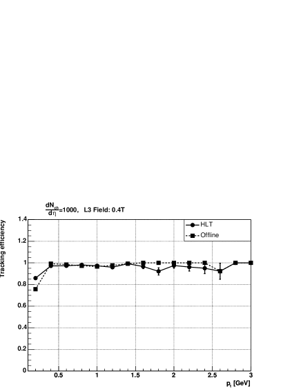
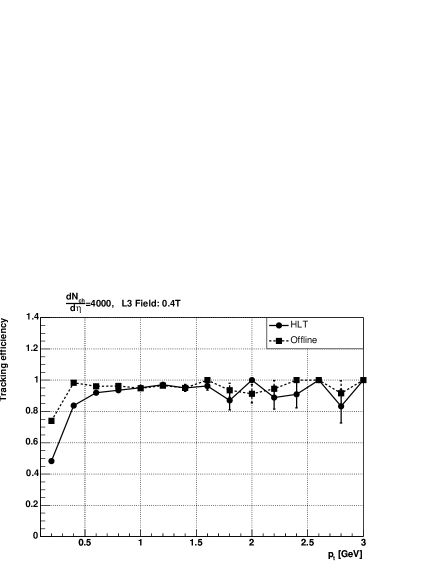
Figure 4.7: Tracking efficiencies as a function of $p_{t}$. Results using magnetic field strength of 0.2 T (left) and 0.4 T (right).

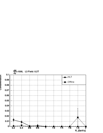
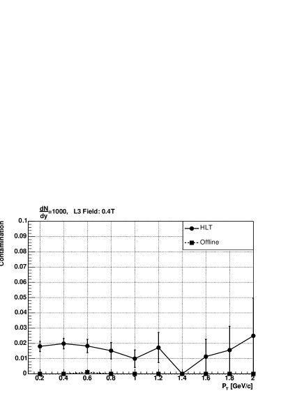
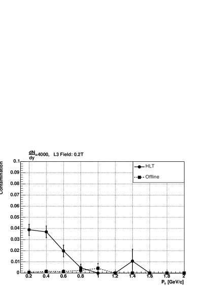
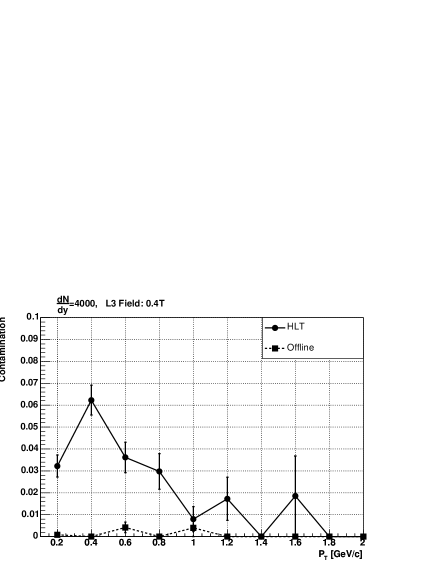
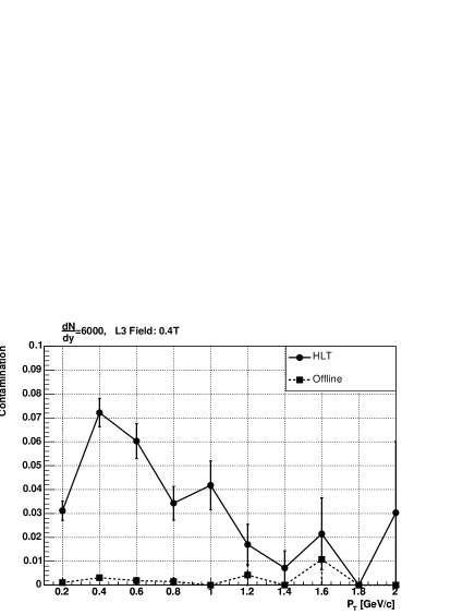
Figure 4.8: Contamination as a function of $p_{t}$. Results using magnetic field strength of 0.2 T (left) and 0.4 T (right).

For a magnetic field strength of 0.2 T the efficiency shows no significant dependence on the transverse momentum at lower multiplicities. At dN_ch/d$\eta$ = 6000, however, a decrease of the low momentum efficiency is observed. This decrease is not seen in the Offline efficiency. For a field strength of 0.4 T, a decrease is seen for the low $p_{t}$ component for both HLT and Offline for all multiplicities. However, the tendency is more significant for the HLT results when going towards higher multiplicities. Up to dN_ch/d$\eta$ = 2000, HLT and Offline results are similar, while for dN_ch/d$\eta$ = 4000 and 6000 the low $p_{t}$ efficiency for HLT is significantly lower than corresponding Offline results.

Figure 4.9 shows the resulting integral efficiency and contamination as a function of multiplicity for both magnetic field strengths. An obvious similarity is seen in the results obtained with the two tracking approaches for multiplicities $\leq$ 2000 for both field settings. For higher multiplicity, the efficiency of HLT algorithms is partially lost to contaminated tracks whose relative amount reaches 4-5% for dN_ch/d$\eta$ = 4000-6000.

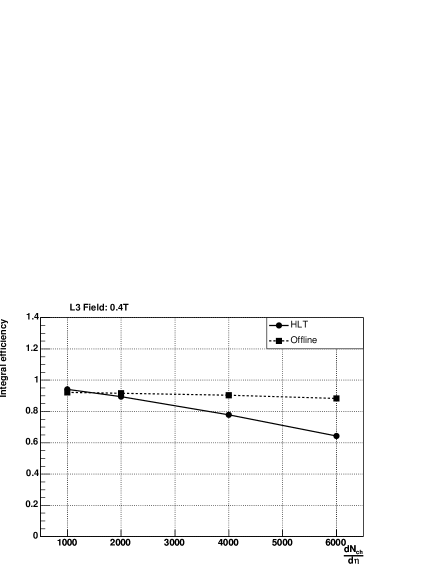
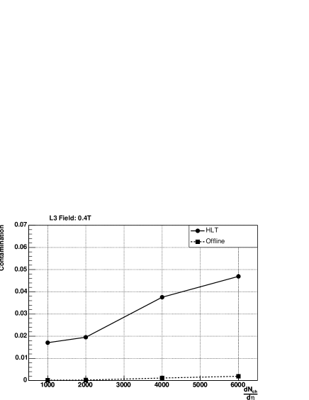
Figure 4.9: Integral efficiency and contamination as a function of multiplicity.

Position resolution

The position resolution can be estimated by calculating the distance, $\delta$, from each space point on a track to the respective trajectory defined by the track fit. The width of the resulting distribution of these residuals can be taken as a measure of the position resolution of the tracks. In Figure 4.10 such a distribution is shown for the transverse and longitudinal direction for a multiplicity of dN_ch/d$\eta$ = 1000. Only tracks with small dip-angle ($|\lambda|\leq 5^{\circ}$) are taken into account for the longitudinal residuals, while all tracks with $p_{t}\geq$ 0.1 GeV are included for the transverse residuals. The distributions include both inner and outer sectors of the TPC, and is thus averaged over the three different pad-geometries. The resolution represented by the RMS-values of the distributions is about 1.37 mm and 1.47 mm for the pad and time direction, respectively. In Figure 4.11 the obtained position resolutions are plotted as a function of multiplicity. Here also the corresponding results from Offline is shown. The results shows a clear deterioration of the resolution in both directions for increasing multiplicities. Similar effect is seen for Offline, although in this case the dependency on multiplicity is less significant.

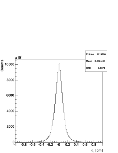
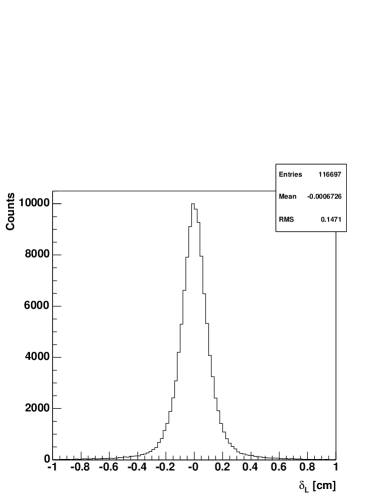
Figure 4.10: Distribution of transverse (left) and longitudinal (right) residuals for dN_ch/d$\eta$=1000. The distributions includes clusters from both the inner and outer TPC readout chambers.

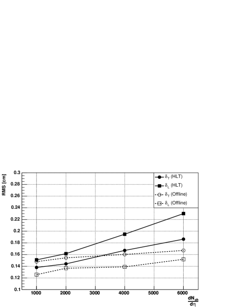
Figure 4.11: Residuals as a function of multiplicity. The results are obtained from the RMS-value of the respective distributions.

Momentum resolution

The momentum resolution of the reconstructed tracks can be estimated by comparing the reconstructed momentum with the momentum of the corresponding simulated particle. The resolution is a function of $p_{t}$, Equation 4.3, and the relative $p_{t}$ resolution is defined as,

$$\Delta_{r}p_{t}=\frac{\Delta p_{t}}{p_{t}}=\frac{p_{t,\mathrm{measured}}-p_{t,\mathrm{particle}}}{p_{t,\mathrm{particle}}},$$ (4.16)

where $p_{t,\mathrm{measured}}\$ is the reconstructed transverse momentum of the track, and $p_{t,\mathrm{particle}}\$ is the transverse momentum of the corresponding simulated particle. In order to measure this quantity for a given sample of tracks, a Gauss-fit of the distribution is commonly performed and the resulting width is taken as a measure of $\Delta_{r}p_{t}$, see example in Figure 4.12. The results for the different event samples are shown in Figure 4.13 as a function of $p_{t}$.

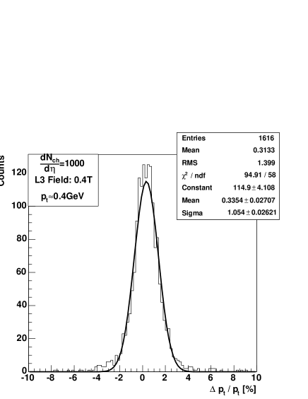
Figure 4.12: Relative transverse momentum resolution for tracks with $p_{t}$ $\approx$0.4 GeV. The distribution is fitted with a Gauss function, that gives a relative width of 1.05%. The distribution is not completely symmetrical, because the measured momentum is inversely proportional to the curvature of the track.

For the low multiplicity regime the relative resolution is contained within the interval 1.5-2.5%, with an average of 1.8% for magnetic field of 0.2 T over the entire $p_{t}$ range. For a magnetic field of 0.4 T the resolution is centered around 1.2% for the same multiplicity. The difference between HLT and Offline results in this regime is small. For higher multiplicities the difference between HLT and Offline becomes more significant, in particular in the higher $p_{t}$ range.

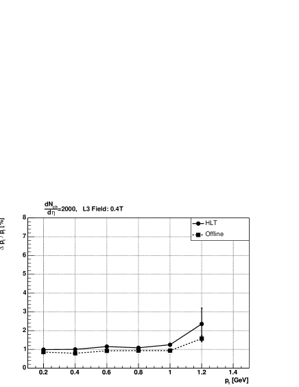
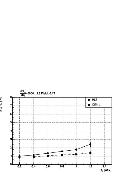
Figure 4.13: Relative transverse momentum resolution as a function of $p_{t}$. Results obtained using magnetic field strength of 0.2 T (left) and 0.4 T (right), respectively.

Remarks on the observed tracking performance

In summary, the results from these simulations indicates a significant loss of tracking performance in the low momentum regime for higher multiplicities. These efficiencies may be explained by several factors. The main reason for the efficiency loss seen for the HLT reconstruction chain compared to the Offline results is the quality of the reconstructed clusters. The Cluster Finder algorithm follows a rather simple sequence matching scheme, and implements a straight-forward center-of-gravity approach to obtain the cluster centroids. Due to the fact that the Cluster Finder has no prior information about the individual charge distributions, overlapping clusters are not handled very well. As a consequence, overlapping clusters are split wrongly and the centroid calculations are biased. This is also reflected in the observed deterioration of the space point resolution as a function of multiplicity (Figure 4.11). In addition, a number of noise clusters may also be wrongly identified from very low $p_{t}$ tracks or $\delta$-electrons which produce rather large areas of continuous signal in the pad-row planes. These areas are interpreted by the Cluster Finder as many overlapping clusters. Both these effects contribute to the local track follower getting dis-oriented during cluster assignment. As a result tracks are being split and contaminated by wrongly assigned clusters.

Furthermore, the track finding procedure reconstructs tracks based on a simple fit selection criteria in conformal space, and does not include more advanced correction for energy loss and multiple scattering. Since the impact of multiple scattering and energy loss is higher for low energy particles, this effect is more significant in the low momentum regime.

Parts of the efficiency loss at low momentum and high field setting may also be explained by the fact that the Track Finder is implemented in a parallel fashion, i.e. the tracks are reconstructed at the TPC sector level. Consequently, the tracks which cross the sector boundaries have to be merged by the subsequent Track Merger. If the quality of the individual track segments are poor and the track density is high, the Track Merger may not be able to correctly merge the corresponding track segments.

Secondary tracks

The tracking performance discussed above were determined exclusively for primary tracks. In order to get an estimate of the reconstruction capabilities of secondary particles, a complementary was done including a selection of secondary particle tracks. In this case the generated good tracks in Equation 4.15 was defined as particles which are decay products of $K$ and $\Lambda$ particles. In addition, the respective tracks are required to be contained within the TPC acceptance and furthermore cross at least 40% of all padrows (same requirement as was made for the primary tracks above). The selected particles thus consists of

$$K : \ \mu,\ e,\ \pi$$

$$\Lambda : \ p,\ \pi$$

for the two cases respectively.

In this case, a second pass was done during the track finding step, where the second tracking pass took the unused clusters from the first pass as input. As explained previously, no vertex constraint was imposed on these secondary tracks, and thus the conformal mapping of the space points was calculated relative to the first assigned cluster to a track. In Figure 4.14 the resulting efficiency as a function of $p_{t}$ is shown for events with multiplicity of dN_ch/d$\eta$ = 1000. For reason of comparison, the efficiency obtained with an recently developed version of the Offline chain is also shown. This new Offline approach consists of an improved Kalman filter [71] which includes optimization for detection of secondaries. The tracking efficiency is $\sim$60% for the low momentum bin, while at higher $p_{t}$ it increases to $>$80%. The difference between Offline and HLT is significant at the low momentum, whereas the difference decreases at higher momentum. It should be noted that the current HLT algorithm was not tuned for the detection of secondary tracks with the exception of the second tracking pass adaption.

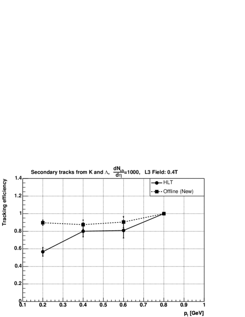
Figure 4.14: Tracking efficiency of secondary tracks from decay of $K$ and $\Lambda$ particles using HLT (solid line) and an improved Offline chain (dotted line).

Computing requirements

The computing requirements of the various processing tasks can be estimated by measuring the CPU time needed for the different processing modules. Such measurements may indicate the amount of computing power needed to implement the algorithm to run on the High Level Trigger system, and in particular which processing steps represent the bottlenecks. In the same way as the tracking performance depends on the particle multiplicity, the required processing time is correlated with the number of space points and tracks which have to be reconstructed.

The processing time of all the individual process components was measured for various event multiplicities. For the test, a standard PC consisting of a 800 MHz Twin Pentium III with a Serverworks Chipset, 256 kB L2 Cache running a Linux kernel v2.4 was used. All measurements were performed while the data was located within the memory, i.e. no overhead from any external device access (disk, network interface etc.) was included. The left plot in Figure 4.15 shows the measured processing times for three different multiplicities. The measurements are resolved with respect to the different computing steps, where the values corresponds to the time needed by a single processing module as implemented in the scheme shown in Figure 4.6. For instance, for a multiplicity of dN_ch/d$\eta$ = 1000 the Cluster Finder needs on average about 8 ms to process the pad-rows which is contained within a single sub-sector, while the Track Finder needs about 130 ms to reconstruct the track segments within a complete TPC sector. The Track Finder step includes both the transformation of the space points into conformal space and the track following procedure.

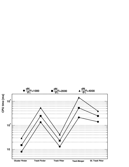
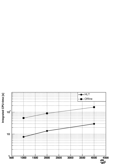
Figure 4.15: Compute time requirements measured on an 800 MHz processor for three different particle multiplicities. Measured CPU-time for the sequential tracking chain resolved with respect to the different processing steps (left). Measured CPU-time integrated over all the processing steps performed sequentially on a single CPU (right). For reason of comparison the corresponding CPU-time measured for the Offline reconstruction chain is shown (dotted line).

In the right plot in Figure 4.15 measured CPU-time integrated over all the processing steps performed sequentially on a single CPU is shown as a function of multiplicity. The measured CPU-time needed by the Offline reconstruction chain is also shown. For the Offline reconstruction chain, data loading into memory is included in the measurement, as no clear separation between loading and processing of data is available in its current implementation. At dN_ch/d$\eta$ = 4000 the HLT chain needs a total of about 30 s to for a full TPC event reconstruction, while Offline needs about 170 s.

4.6 Iterative Tracking

In the sequential tracking approach described in the previous section, the cluster centroids are obtained using a straight-forward center-of-gravity calculation. Such an algorithm has obvious limitations when applied to a high occupancy environment, since the lack of information about the tracks bias the centroid calculation in the case of overlapping charge distributions. The main objective of iterative tracking is to provide the track information prior to the cluster finding in order to better fit and unfold the overlapping clusters. From this the correct cluster centroids should be obtained.

In this approach, the pattern recognition scheme consists of two main parts: Track candidate finding and cluster fitting. In a first step an implementation of the Hough Transform is applied to the raw ADC-data in order to obtain a list of track candidates. These track segments serve as input for the Cluster Fitter, which reconstructs the cluster centroids along the particle trajectories by fitting the respective charge distributions to a parameterized shape. Finally, the assigned clusters are fitted to a helix in order to obtain the best estimate of the track parameters.

4.6.1 The Cluster Fitter

The implemented fitting routines were initially developed for TPC data in the NA49 experiment [47]. It assumes that the clusters can described using a two-dimensional Gauss function.

The cluster model

The shape of the clusters is given by the convolution of the response functions of the readout pads, Section 2.4.1. Both the pad and time response functions have a close to Gaussian shape, as well as the spread of the electron clouds due to diffusion. The cluster model can thus to a good approximation be described with a two-dimensional Gauss-distribution whose widths depend on geometry of the pads and the track parameters. A total of five independent parameters are needed to fully describe the model:

• The two-dimensional position $(p,t)$ in pad and time direction.

• The widths $(\sigma_{\mathrm{pad}},\sigma_{\mathrm{time}})$, in pad and time.

• The amplitude of the distribution.

These parameters vary for each cluster, so without any prior knowledge they would all have to be fitted for. In the case of overlapping clusters such a fitting procedure would be a very demanding task as no information about the number of contributing tracks, nor the shape for each individual charge distributions, is known. The shape of the clusters in the TPC depends on the drift length (diffusion of the drifting electrons in the gas), and track crossing angles with the pad-row-plane (spread of primary ionization electrons), and can be parameterized according to [49]:

$$\sigma_{\mathrm{pad}}^{2} = \sigma_{PRF}^{2}+D_{T}^{2}\cdot s_{\mathrm{drift}}+\frac{l^{2}\cdot\tan^{2}(\beta)}{12}+\frac{d^{2}\cdot(\tan(\alpha)-\tan(\psi))^{2}}{12}$$

$$\sigma_{\mathrm{time}}^{2} = \sigma_{0}^{2}+D_{L}^{2}\cdot s_{\mathrm{drift}}+\frac{l^{2}\cdot\tan^{2}(\lambda)}{12}$$ (4.17)

where the various terms are described in Section 2.4.1, page 2.4.1. This parameterization indicates that any prior knowledge of track parameters could provide the fitting procedure with an improved initial guess of the parameters, or even reduce the number of parameters to vary in a fit.

Although the average cluster widths can be described with the parameterization in Equation 4.17, their properties are determined by stochastic processes and are thus also subject to fluctuations. The fluctuation of the shape depends on the contribution of the random diffusion and angular spread of the ionization, and also on the gas gain fluctuations and secondary ionization.

Fitting procedure

The implemented procedure fits the clusters to the model

$$q(p,t)=\sum_{k=1}^{K}A_{k}\exp\left[-\frac{1}{2}\left(\frac{p-p_{k}}{\sigma_{\mathrm{pad},k}}\right)^{2}-\frac{1}{2}\left(\frac{t-t_{k}}{\sigma_{\mathrm{time},k}}\right)^{2}\right]$$ (4.18)

which is a sum of $K$ two-dimensional Gauss-distributions, with the variables $A_{k}$, $(p_{k},t_{k})$ and $(\sigma_{\mathrm{pad},k},\sigma_{\mathrm{time},k})$ denoting the amplitude, position and widths of the individual distributions, respectively. A $\chi^{2}$ fit of the model to the cluster data is done by applying the Levenberg-Marquardt method [76] to minimize the least square error in the fit. All five parameters may be free to vary in the fit, or only a subset of them may be fitted while the rest are held fixed at their input values. In either case, the fitting routine returns the best fit values for the free parameters in the fit. Once each cluster has been fitted to a Gaussian distribution, the total charge of the cluster can be obtained from the relation

$$Q_{\mathrm{total},k}=2\pi\sigma_{\mathrm{pad},k}\sigma_{\mathrm{time},k}A_{k}.$$ (4.19)

The procedure can also be extended to other models for the cluster shape, e.g. to account for asymmetric Gaussian distributions. In that case the two-dimensional Gaussian given above may be replaced with an alternative model, and the fitting procedure is done accordingly.

Deconvolution of overlapping clusters

In the case of overlapping clusters, $K\geq 2$, the corresponding charge distribution is fitted to a sum of $K$ individual Gauss-distributions. If the track parameters are known from a preceding pattern recognition step, all 5$\times K$ parameters may be provided with initial values. In addition, deconvolution can now be done by fixing the widths of the individual distributions and only letting the positions and the amplitude parameters vary freely.

An example of deconvolution of two overlapping clusters is shown in Figure 4.16.

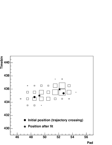
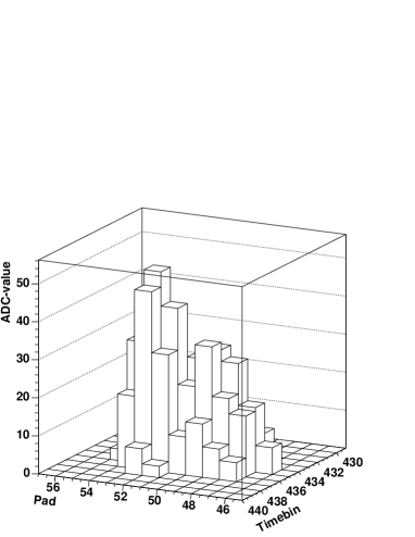
Figure 4.16: Illustrating fitting and deconvolution of overlapping clusters. Left: The circles mark the initial position given as input to the fitting routine, while the star marks the best-fit values returned from the fit. Right: Same clusters shown using a lego-plot.

In this case the input to the fitting routine are the two sets of 5 initial parameters, each consisting of the position in the pad-row-plane (illustrated by the circle markers), the widths of the distribution in two dimensions and the amplitude. The initial values of these parameters are determined from the results obtained by the preceding tracking finding algorithm. The initial positions are taken as the crossing point of the computed tracks with the pad-row-plane, while the widths are calculated from Equation 4.17 with the track inclination angles and initial positions as input. During the fitting procedure, the widths are kept fixed at their input values, while the remaining parameters are free to vary. This means that in this case there are 3+3 parameters which are being fitted for. The fitting routine finally returns the best-values obtained for each position (illustrated by the star markers) and the respective amplitudes of the individual distributions. In this way the initial positions serve as the prediction of the cluster centroids, while the returned values from the fit are the corrected, final reconstructed cluster centroids. The improved parameter estimates are subsequently returned to the track model.

Figure 4.17: Flow diagram of the Cluster Fitter algorithm.

The algorithm

The implemented Cluster Fitter algorithm assumes that the track parameters have been obtained by a preceding track finding algorithm, and thus takes a list of track candidates as input. In a first step each input track is propagated through the TPC detector and the intersection between the helical trajectories and the pad-row-planes is calculated and stored internally for each track candidate.

The algorithm then processes each pad-row separately as illustrated by the flow diagram in Figure 4.17. A loop is performed over all track intersection points with the current pad-row. For each track, a region around its intersection point in the pad-row-plane is searched for a nearest cluster. In addition, any potential additional tracks contributing to the given cluster is identified. If a local maxima is found within the cluster distribution, the clusters are fitted. A track candidate is only taken into account in the fit if it can be associated with a local maxima in the distribution. The reason for this criteria is to avoid taking into account fake tracks, i.e. tracks which may have been falsely identified as a track candidate during the preceding track procedure. If the resulting fit returns an acceptable $\chi^{2}$ the clusters are stored with the values obtained in the fit, otherwise the clusters are removed. During the fit the widths are always held fixed at their input values, while the position and amplitude are fitted for.

In Table 4.3 the space point resolutions achieved with the Cluster Fitter are listed for both isolated ($K$=1) and overlapping clusters ($K\geq$ 2). The input parameters to the fit were in this case provided by the respective simulated particle trajectory producing the cluster.

	Pad direction [mm]		Time direction [mm]
$K$=1	Gauss-fit	CoG	Gauss-fit	CoG
Inner chambers	0.97	0.99	1.48	1.33
Outer chambers	0.90	0.88	1.27	1.14
$K\geq$2
Inner chambers	1.90	2.90	2.33	3.54
Outer chambers	1.78	4.68	1.92	4.36

Table 4.3: Comparison of the space point resolution obtained by applying the fitting procedure and the center-of-gravity (CoG), corresponding to the Cluster Finder, on both isolated ($K$=1) and overlapping ($K\geq$ 2) clusters.

For comparison, the corresponding resolutions achieved using the Cluster Finder in the sequential tracking scheme (Section 4.5.1) are also listed. The results show that for isolated clusters the transverse resolution obtained in the two approaches are similar, while the longitudinal resolution is slightly worse in the fitting approach. In the case of overlapping clusters, the Cluster Fitter achieves 30-50% better resolution compared to the Cluster Finder.

4.6.2 The Hough Transform

The Hough Transform (HT) is a widely adapted algorithm in image analysis related fields. Originally it was used to recognize linear patterns in binary images [60], but the principle can easily be implemented to any kind of pattern. A complete review of HT methods and main developments can be found in e.g. [77] and [78].

The basic idea of the HT is easily understood by considering a straight line, $y=ax+b$, where the parameters $a$ and $b$ define the slope and intercept respectively. The HT uses the idea that this equation can be reformulated into $b=-ax+y$. Thus a point ($x,y$) is seen to define a straight line in a two-dimensional parameter space. In the space of parameters $a$ and $b$, this line corresponds to all possible straight lines going through the point $(x,y)$ in the $xy$-plane. If several points $(x_{i},y_{i})$ are along a straight line in the $xy$-plane, the transformed lines in parameter space will intersect at the point $(a,b)$ which defines the actual parameters of the line. By identifying this point of intersection, one has identified the line itself. Thus the effect of the HT is to reduce the recognition of global patterns in a image space to a local peak detection in parameter space. This is illustrated in Figure 4.18.

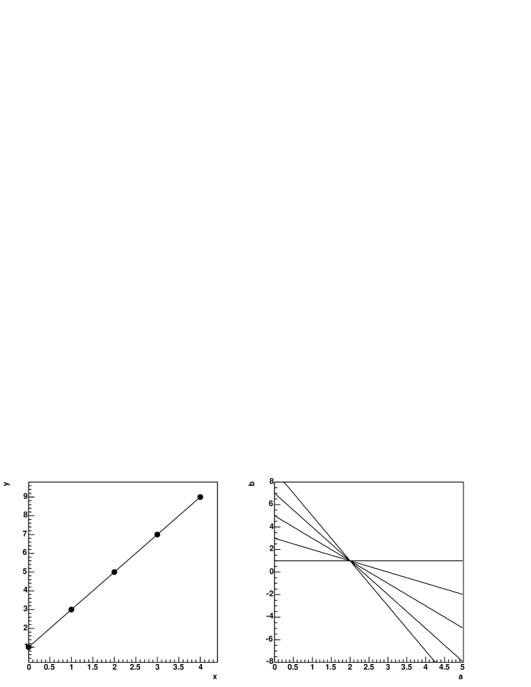
Figure 4.18: Illustration of a simple HT applied to points lying on the straight line $y=2x+1$ (left). Each point transforms to a line in the parameter space (right), and the intersection of these lines defines the parameters of the line.

Formally one can describe the transform as follows. Let $X\$ be a point in image space and $\Omega$ a point in parameter space. A set of image points which lie on a curve can then be defined by the function $f$ such that

$$f(X,\Omega)=0.$$ (4.20)

In the case of a straight line one can define $X$=$(x,y)$ and $\Omega=(a,b)$. The equation for a straight line then becomes $f(X,\Omega)=y-ax-b=0$ and maps each value of the parameter combination $(a,b)$ to a set of image points. The mapping is one to many from the space of possible parameters values to the space of image points. Equation 4.20 can be viewed as a mutual constraint between image points and parameter points and therefore it can be interpreted as defining a mapping from a set of image points to a set of possible parameter values.

The HT can be defined for arbitrary parametrically defined image curves. When considering curves characterized by $N$ parameters, the HT will map out of hyper-surface in a $N$-dimensional parameter space. Correspondingly the intersection of these surfaces marks a possible candidate for the curves in image space. The HT for a set of image points, $\{X_{1},X_{2},...,X_{n}\}$, is defined as

$$H(\Omega)=\sum_{j=1}^{n}p(X_{j},\Omega)$$ (4.21)

where

$$p(X,\Omega)=\left\{\begin{array}[]{ll}1&\mbox{if $f(X,\Omega)=0$}\\ 0&\mbox{otherwise}\end{array}\right.$$ (4.22)

In practical implementations of the HT, the continuous parameter space is usually considered to be composed of the union of finite-sized regions. One then makes parameter space discrete and defines a counter for each cell in the parameter space. Each cell is associated with a element in a multi-dimensional array, and the respective counters are incremented when a hyper-surface from the transform of an image point passes through the region of parameter space associated with the element. This array is in literature referred to as the Hough accumulator array. If C_Ω denotes a element in the accumulator array which corresponds to a cell in the parameter space centered at $\Omega$, then consequently $p(X,\Omega)$ is 1 if any curve corresponding to the parameter space cell C_Ω passes through the point, $X$, in image space. This can be considered as every image point giving “votes” to all the possible parameter combinations it can possibly belong to. The detection of the intersection of the surfaces is done by detection of local peaks in the number of accumulator counts. The size and shape of these peaks depend on several factors, such as the number of transformed image points, the errors of the image points and the size of the parameter cells.

The standard Hough transform as described above is a divergent transform, i.e. a point is mapped onto a curve in parameter space. It is however possible to reformulate the transform so that it becomes a convergent transform. In this case, instead of transforming single image points into curves in parameter space, subset of points is mapped. The advantage of this approach is that each mapping is into a smaller subset of the parameter space. However, since all combinations of possible subsets of image points has to be mapped in the transform, the combinatorics of such algorithm makes it very computing intensive.

Implementation issues

As described in the previous section, the underlying idea of the HT is to search for some kind of predefined parameterized pattern in an certain image space. In the case of the ALICE TPC, the image space consists of the digitized charge distributions sampled from the ionization along the particle trajectory, while the patterns to be parameterized are defined by the motion of the charged particles in the homogeneous magnetic field. The main implementation issues of such an algorithm consists of defining a proper parameterization and its corresponding HT, together with the adaption of a optimal parameter space. These issues are discussed in the following.

Parameterization and derivation of the HT

A charged particle which moves in a homogeneous magnetic field follows a helical trajectory. This corresponds to a circular motion in the plane perpendicular to the magnetic field, and a non-curved motion in the plane along the magnetic field. In total five independent parameters are needed to fully describe the helix in three dimensions (Appendix A.2). Under the assumption that the helix originates from the vertex, the following parameterization can be used,

$$x(t) = \frac{1}{\kappa}\{\sin(\psi_{0}+ht)-\sin\psi_{0}\}$$

$$y(t) = \frac{1}{\kappa}\{-\cos(\psi_{0}+ht)+\cos\psi_{0}\}$$

$$z(t) = \gamma t,$$ (4.23)

where $\kappa$ is the curvature, $\psi_{0}$ is the emission angle with the x-axis, $h$ is the sense of rotation, $\gamma$ governs the longitudinal translation and $t\in[0,\pi]$. In this scenario the number of required parameters are reduced to the 3 independent parameters, $(\kappa,\psi_{0},\gamma)$, where the two former describe the circle in the transverse plane and the latter the straight line in the longitudinal plane.

Now let $X_{i}=(x_{i},y_{i},z_{i})$ denote a point lying on the helix, and $\Omega$ = $(\kappa,\psi_{0},\gamma)$ the parameters of a helix. Following the terminology introduced above, $X_{i}$ and $\Omega$ represent points in image space and parameter space respectively. Let $M_{i}(X_{i},\Omega)$ denote the minimal squared distance between a helix and a point $i$,

$$M_{i}(X_{i},\Omega)=M_{i}^{xy}+M_{i}^{z}=(x_{i}-x)^{2}+(y-y_{i})^{2}+(z-z_{i})^{2},$$ (4.24)

where $M_{i}^{xy}$ and $M_{i}^{z}$ denote the transverse projection and the longitudinal distance respectively. In order to derive the standard HT for this helix parameterization one has to solve the equation

$$M_{i}(X_{i},\Omega)=0.$$ (4.25)

This formula allows the determination of the set of all helix parameters which correspond to the given point $X_{i}$. The transformation defines a mapping of one point in our image space into a three dimensional curve in the parameter space span by $(\kappa,\psi_{0},\gamma)$. The problem can be simplified by considering the transverse and the longitudinal part of the helix separately:

$$(x,y) \leftrightarrow (\kappa,\psi_{0})$$

$$(z) \leftrightarrow (\gamma)$$

The transform in the transverse plane is then defined by the equation $M_{i}^{xy}$=0, and and maps the transverse projection of a point into a curve in the two-dimensional parameter space span by $(\kappa,\psi_{0})$. In the latter case the transform is defined by $M_{i}^{z}$=0 and maps a point into a one-dimensional parameter space span by $\gamma$.

Substituting $x$ and $y$ from Equation 4.23 into $M_{i}^{xy}$ in Equation 4.25 gives

$$\frac{1}{\kappa^{2}}\left\{1-\sqrt{(\kappa x_{i}+\sin\psi_{0})^{2}+(\kappa y_{i}-\cos\psi_{0})^{2}}\right\}^{2}=0.$$

Taking the square root and changing to polar coordinates ($x_{i},y_{i})\rightarrow(r_{i},\phi_{i})$ gives

$$\pm\frac{1}{\kappa}\left\{1-\sqrt{\kappa^{2}r_{i}^{2}+2\kappa r_{i}(\cos\phi_{i}\sin\psi_{0}-\sin\phi_{i}\cos\psi_{0})+1}\right\}=0$$

$$\frac{1}{\kappa}\left\{-\kappa^{2}r_{i}^{2}+2\kappa r_{i}\sin(\phi_{i}-\psi_{0})\right\}=0$$

which finally gives the expression

$$\kappa=\frac{2}{r_{i}}\sin(\phi_{i}-\psi_{0})$$ (4.26)

Equation 4.26 is thus the standard HT for the parameterization of a helix going through (0,0) projected into the transverse plane. According to this transform a single image point will by mapped into a sinusoidal curve in parameter space.

Similarly, substituting $z$ from Equation 4.23 gives

$$\gamma=\frac{z_{i}}{t}.$$ (4.27)

This transform thus corresponds to a mapping into a one-dimensional parameter space span by $\gamma$.

Equations 4.26 and 4.27 defines the HT for the transverse and longitudinal pattern of the helix parameterization in Equation 4.23. Using this definition two separate accumulator arrays are required which can be denoted as $H(\kappa,\psi_{0})$ and $H(\gamma)$ respectively. The two sets are correlated, i.e. a valid peak in $H(\kappa,\psi_{0})$ will have a corresponding peak in $H(\gamma)$. This can be utilized by defining subsets in $\gamma$, and thereby transforming all points located within a given subset into $H(\kappa,\psi_{0})$. A helix whose points are confined within the subset, will consequently create a peak in $H(\kappa,\psi_{0})$ corresponding to the parameters of the helix in the transverse plane. The longitudinal parameter of the helix can thus be determined from the values of the subset being transformed. For the purpose of defining such sub-volumes, the pseudo-rapidity, $\eta$, has been used. This is a geometrical quantity defined by the angle between the trajectory and the beam axis, $\theta$, as

$$\eta=\ln(\tan\frac{\theta}{2})^{-1}.$$ (4.28)

$\theta$ is related to the dip-angle of the track, $\lambda$, as $\theta=\frac{\pi}{2}-\lambda$. The pseudo-rapidity of a image point $(x,y,z)$ is defined as

$$\eta=\frac{1}{2}\ln\frac{r_{3}+z}{r_{3}-z}$$ (4.29)

where $r_{3}=\sqrt{x^{2}+y^{2}+z^{2}}$. The standard HT (Equation 4.21) for a set of image points, $\epsilon_{k}=\{X_{1},X_{2},...,X_{n}\}$, is then defined as

$$H_{k}(\kappa,\psi_{0})=\sum_{j=1}^{n}p(x_{j},y_{j},\kappa,\psi_{0})$$ (4.30)

where

$$p(x,y,\kappa,\psi_{0})=\left\{\begin{array}[]{ll}1&\mbox{if $\kappa=\frac{2}{r}\sin(\phi-\psi_{0})$}\\ 0&\mbox{otherwise}\end{array}\right.$$ (4.31)

and

$$\epsilon_{k}\in[\eta_{k},\eta_{k+1}]$$ (4.32)

$\epsilon_{k}$ corresponds to the set of points located within a sub-volume in the longitudinal plane, Figure 4.19. Each sub-volume thus defines an image space which contains circular patterns corresponding to the projected tracks in the transverse plane.

Figure 4.19: Definition of the image space in the HT. The image space (right) is defined as a sub-volume characterized by the pseudo-rapidity, $\eta_{k}$ (left).

On choosing the quantization scheme for $H(\kappa,\psi_{0})$

To compute the HT both the ranges and the quantization steps must be selected for $H(\kappa,\psi_{0})$. The proper choice of these parameters is an essential part of the algorithm as they directly affect the memory size, processing times and the final accuracy of the obtained track parameters. The optimal number and size of bins in the parameter space depend generally on aspects like the number and density of the data points, the required resolution, the noise level and computing requirements. For example, choosing a bin size which is too big will restrict the achievable resolution on the reconstructed tracks. On the other hand, if the bin size is too small the image points on a single track will be spread throughout too many bins and may not create a distinct peak at all.

In order to choose the set of properties for the parameter space, an investigation of the characteristics of the formed peak is necessary. The shape and size of the peak is determined by two main factors: The sampling of the parameter space, and the “noise” of the image points. In this context noise includes all factors which contribute to the image points not being perfectly aligned on the circle parameterization, and consequently would lead to the intersection point in parameter space being smeared over a finite area.

The intrinsic accuracy of the transform is limited by the sampling intervals chosen for the accumulator array, $H$. Moreover, the formation of peaks in the parameter space is directly influenced by how the space is quantized.

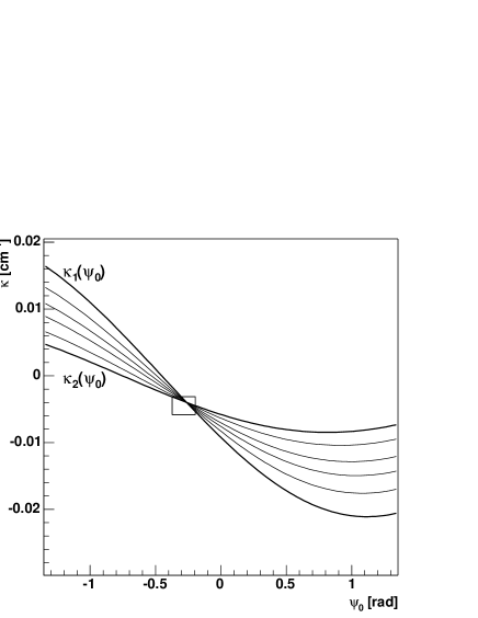
Figure 4.20: Peak formation in the HT parameter space. The transformation of the points lying in a circular segment define sinusoids in the parameter space (left). The curves corresponding to two end-points on the segment are denoted $\kappa_{1}$ and $\kappa_{2}$. The peak is spread due to the sampling of the parameter space (right).

Following the procedure introduced in [79] one can investigate the effect on formation of the peaks in the parameter space. Consider an ideal circular trajectory defined by the parameters $(\kappa_{t},\psi_{0,t})$ with two points $(r_{1},\phi_{1})$ and $(r_{2},\phi_{2})$ as illustrated in Figure 4.19. These two points will under the HT define two sinusoids in the parameter space, $H(\kappa,\psi_{0})$ (Figure 4.20, left),

$$\kappa_{1}(\psi_{0}) = \frac{2}{r_{1}}\sin(\phi_{1}-\psi_{0})$$

$$\kappa_{2}(\psi_{0}) = \frac{2}{r_{2}}\sin(\phi_{2}-\psi_{0}),$$ (4.33)

with the derivatives

$$\frac{\partial\kappa_{1}}{\partial\psi_{0}} = -\frac{2}{r_{1}}\cos(\phi_{1}-\psi_{0})$$

$$\frac{\partial\kappa_{2}}{\partial\psi_{0}} = -\frac{2}{r_{2}}\cos(\phi_{2}-\psi_{0}),$$ (4.34)

In addition, let $(r_{0},\phi_{0})$ represent a point on the circle between the two points. Assuming that $|\phi-\psi_{0}|<\pi/2$ and $r_{1}<r_{0}<r_{2}$ gives

$$\kappa_{1}(\psi_{0})>\kappa_{0}(\psi_{0})>\kappa_{2}(\psi_{0})\hskip 14.22636pt\mbox{for $\psi_{0}<\psi_{0,t}$}$$

$$\kappa_{1}(\psi_{0})<\kappa_{0}(\psi_{0})<\kappa_{2}(\psi_{0})\hskip 14.22636pt\mbox{for $\psi_{0,t}<\psi_{0}$}$$ (4.35)

The peak formed by the transformation exhibits a typical cross shape (Figure 4.20, right), where the spread will be confined by the the curves of $\kappa_{1}$ and $\kappa_{2}$. Let now $\psi_{0}$ be sampled with a uniform interval $\Delta_{q}\psi_{0}$ and assume that $\psi_{0,t}$ lies between $\psi_{0,k}-\frac{1}{2}\Delta\psi_{0}$ and $\psi_{0,k}+\frac{1}{2}\Delta\psi_{0}$ where $k\in[0,m]$. The uncertainty between $\psi_{0,k}$ and $\psi_{0,t}$ can be given by

$$-\frac{1}{2}\Delta_{q}\psi_{0}\leq\delta\psi_{0,k}=\psi_{0,t}-\psi_{0,k}\leq\frac{1}{2}\Delta_{q}\psi_{0}.$$ (4.36)

Each of the accumulators can be regarded as small rectangular window overlaid the continuous parameter space. Assume that the true peak is located within the window of size $\Delta_{q}\psi_{0}\times\Delta_{q}\kappa$ with center $(\psi_{0,k},\kappa_{h})$ where $h\in[0,n]$. The uncertainty between $\kappa_{h}$ and $\kappa_{t}$ is then

$$-\frac{1}{2}\Delta_{q}\kappa\leq\delta\kappa_{h}=\kappa_{t}-\kappa_{h}\leq\frac{1}{2}\Delta_{q}\kappa.$$ (4.37)

Depending on the relative size of $\Delta_{q}\psi_{0}$ and $\Delta_{q}\kappa$, the peak will be distributed or spread out over several bins in the accumulator array. The total spread in the $\kappa$-direction, $\Delta_{ps}\kappa$ at the sampling interval $\psi_{0,k}$ is given by

$$\Delta_{ps}\kappa(\psi_{0,k})=\kappa_{1}(\psi_{0,k})-\kappa_{2}(\psi_{0,k})$$ (4.38)

Substituting $\delta\psi_{0,k}=\psi_{0,t}-\psi_{0,k}$ gives

$$\Delta_{ps}\kappa(\psi_{0,k}) = \frac{2}{r_{1}}\sin(\phi_{1}-\psi_{0,t}+\delta\psi_{0,k})-\frac{2}{r_{2}}\sin(\phi_{2}-\psi_{0,t}+\delta\psi_{0,k})$$ (4.39)

$$= \cos(\delta\psi_{0,k})\left\{\frac{2}{r_{1}}\sin(\phi_{1}-\psi_{0,t})-\frac{2}{r_{2}}\sin(\phi_{2}-\psi_{0,t})\right\}$$

$$+\sin(\delta\psi_{0,k})\left\{\frac{2}{r_{1}}\cos(\phi_{1}-\psi_{0,t})-\frac{2}{r_{2}}\cos(\phi_{2}-\psi_{0,t})\right\}$$

$$= \cos(\delta\psi_{0,k})\left\{\kappa_{1}(\psi_{0,t})-\kappa_{2}(\psi_{0,t})\right\}$$

$$+\sin(\delta\psi_{0,k})\left\{\left(\frac{\partial\kappa_{2}}{\partial\psi_{0}}\right)_{\psi_{0}=\psi_{0,t}}-\left(\frac{\partial\kappa_{1}}{\partial\psi_{0}}\right)_{\psi_{0}=\psi_{0,t}}\right\}$$

In the last equation the first term equals zero since $\kappa_{1}(\psi_{0,t})=\kappa_{2}(\psi_{0,t})=\kappa(\psi_{0,t})$ which gives

$$\Delta_{ps}\kappa(\psi_{0,k})=\sin(\delta\psi_{0,k})\left\{\left(\frac{\partial\kappa_{2}}{\partial\psi_{0}}\right)_{\psi_{0}=\psi_{0,t}}-\left(\frac{\partial\kappa_{1}}{\partial\psi_{0}}\right)_{\psi_{0}=\psi_{0,t}}\right\}$$ (4.40)

Maximum spreading of the peak occurs when (see Equation 4.37)

$$\mbox{max}(|\delta\psi_{0,k}|)=\frac{1}{2}\Delta_{q}\psi_{0}$$ (4.41)

which yields

$$(\Delta_{ps}\kappa(\psi_{0,k}))_{\mbox{max}}=\sin(\frac{1}{2}\Delta_{q}\psi_{0})\left\{\left(\frac{\partial\kappa_{2}}{\partial\psi_{0}}\right)_{\psi_{0}=\psi_{0,t}}-\left(\frac{\partial\kappa_{1}}{\partial\psi_{0}}\right)_{\psi_{0}=\psi_{0,t}}\right\}$$ (4.42)

Consequently, the following condition on the bin size will allow a maximum collection votes without peak spreading:

$$\Delta_{q}\kappa=(\Delta_{ps}\kappa(\psi_{0,k}))_{\mbox{max}}.$$ (4.43)

Equation 4.43 shows that values of quantization steps combine to influence the spreading of the peak, which indicates that they cannot be selected fully independently. In particular, one can differ between the two cases,

$$\Delta_{q}\kappa < (\Delta_{ps}\kappa(\psi_{0,k}))_{\mbox{max}}$$

$$\Delta_{q}\kappa > (\Delta_{ps}\kappa(\psi_{0,k}))_{\mbox{max}},$$ (4.44)

which can be interpreted as under-sampling and oversampling of $\psi_{0}$ with respect to $\kappa$ respectively. The effect of the former case is to split the votes to neighboring accumulators in the $\kappa$-direction, while the latter corresponds to the case where the peak is distributed over several neighboring bins in the $\psi_{0}$-direction.

This derivation shows that for an ideal circle segment, the resulting peak will be spread with a characteristic form due to the quantization of the parameter space. The implicit assumption is that all the image points on the circle are transformed into a single bin if the proper quantization is chosen. However, the image points, represented by the digitized charge distribution in the TPC detector, do not lie on an ideal circular trajectory due to the energy loss and multiple scattering of the particles and the intrinsic detector noise. As a consequence of the uncertainty of the image points, $(r_{i},\phi_{i})$, on a circular track, the transformation of these points gives a region in the $(\kappa,\psi_{0})$-space rather than a point. The uncertainty of the calculated $\kappa$ can be obtained by taking the Taylor expansion of the transformation Equation 4.26 around $r$ and $\phi$. The first order approximation yields

$$\delta\kappa = \left(\frac{\partial\kappa}{\partial\phi}\right)_{r,\psi_{0}}\delta\phi+\left(\frac{\partial\kappa}{\partial r}\right)_{\phi,\psi_{0}}\delta r$$ (4.45)

$$= \frac{2}{r}\cos(\phi-\psi_{0})\delta\phi-\frac{2}{r^{2}}\sin(\phi-\psi_{0})\delta r.$$

This relation shows that spread of the peak in $\kappa$ is influenced by the noise of image points, but also on the location of the points in the image. Due to the $r^{-2}$ dependence in the second term, the error will be dominated by the error in $\phi$.

In general, the characteristics of the formed peaks in the parameter space depend on both the location of the image points and the track segment in space, and the errors of the individual image points. For a given input image containing several track segments it is therefore generally impossible to quantize $H(\kappa,\psi_{0})$ optimally such that all peaks formed by the transform have the same extension and shape. It is therefore desirable to construct a quantization scheme that as far as possible allows an average peak which keeps a sufficient peak significance with respect to the background.

Accumulation

The HT itself is a pure accumulation procedure. The transformation of each image point consists of incrementing the corresponding counters in a multidimensional array representing the cells in the parameter space. Depending on the nature and topology of the image, different methods can be applied. Many implementations of the HT have suggested using weighting factors so that the most prominent or most certain image features contribute more to the accumulator cells than less certain data. The effect of such schemes is evident: By assigning higher weights to image points lying closer to the parameterization, the corresponding bins will receive a higher vote and will consequently lead to a sharpening of the peaks in parameter space. Formally this is introduced by modifying Equation 4.21 to

$$H(\Omega)=\sum_{j=1}^{n}w(j)p(X_{j},\Omega)$$ (4.46)

where $w(j)$ represents the weighting factor for each image point.

In the case of TPC data, each image point has an associated ADC-value. These values represent the charge distributions of the ionized charge in each pad-row-plane, where the centroid of the distribution denotes the space point of the crossing particle track. In this context, each image point can be regarded as having a certain weight, corresponding to its ADC-value. Thus $w$ in Equation 4.46 is replaced by the ADC-value of the time-bin to be transformed. The implementation of the resulting accumulation algorithm can be illustrated in pseudo-code as follows:

Initialize $H(\kappa,\psi_{0})$ to zero;
for	i:=1 to npoints do
	for	k:=1 to m do
	$\kappa_{t}=\frac{2}{r_{i}}\sin(\phi_{i}-\psi_{k})$;
$\kappa_{h}=Qntz(\kappa_{t},\Delta_{q}\kappa)$;
$H[\psi_{k}][\kappa_{h}]=H[\psi_{k}][\kappa_{h}]$ + ADC-value;
end for
end for

$Qntz()$ denotes the quantizing function which locates the corresponding bin in the $\kappa$-direction. It is thus defined by

$$Qntz(\kappa,\Delta_{q}\kappa)=\left\{\begin{array}[]{ll}\kappa_{p-1}&\mbox{if $\kappa-\kappa_{p-1}\leq\Delta_{q}\kappa/2$}\\ \kappa_{p}&\mbox{otherwise}\end{array}\right.$$

where $p\in[0,m]$.

Each of the accumulator arrays, $H(\kappa,\psi_{0})$, can be interpreted as a two-dimensional histogram, Figure 4.21, where each bin in the histogram corresponds to an element in the accumulator array.

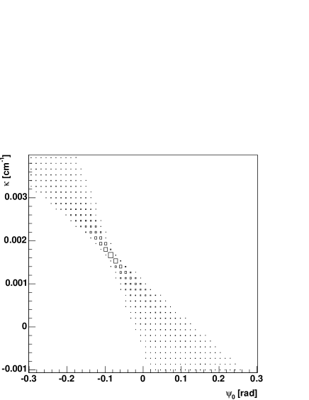
Figure 4.21: Example of the HT parameter space after transforming all points lying along a track with $p_{t}$ =0.5 GeV.

Peak finding

Once the two-dimensional histograms have been filled according to the transformation outlined above, the histograms have to be searched for local peaks which corresponds to potential track candidates. Among these peaks there will in general also be a certain number of false peaks which are originating from artificial features in the image. Such features may e.g. be noisy data points and tracks which are outside the parameter range which is searched. In both cases structural backgrounds are created in the parameter space.

Prior to the peak search, a threshold operation is applied to the histogram. The reason for this is twofold. Firstly, the number of bins which have to be searched by the peak finder, are reduced. Secondly, such a threshold eliminates the contribution from peaks that are too small to correspond to a real track segment. In the simplest case a local peak finder identifies a single histogram bin which corresponds to a local maxima. The requirement for such a local maxima is that it has a value that is larger than its immediate neighbors in the histogram. However, since the shape of the peaks is to the first order known, the peak finder can take advantage of this knowledge in order to better be able to exclude the true peaks from the background.

The goal of the peak finder is to estimate the coordinates of the crossing point, $(\kappa_{t},\psi_{0,t})$, of the peak shape. The implemented procedure starts by locating the initial peaks within a sliding window in the $\kappa$-direction, Figure 4.22. The length of the window, $n_{\kappa}$, is determined by the expected spread of the peak. The idea is thus to choose $n_{\kappa}$ large enough so that it captures the full peak spread in $\kappa$ near $\psi_{0,t}$, and at the same time small enough so that it captures the spread only near $\psi_{0,t}$. If the value of $n_{\kappa}$ is too small the window will not take into account all the transformed points along the track segment, while a window that is too large will include more of the background and may create ambiguities. The complete procedure can be outlined as follows:

1. Location of the initial peaks.
   For each bin in the $\psi_{0}$-direction the sum of values within the sliding window in $\kappa$ is calculated. If a local maxima is found, this window is stored in a temporary list.

2. Location of the two-dimensional peaks.
   Each of the local maxima is compared with the local maxima’s in the neighboring $\psi_{0}$-bins in order to validate the peak in the two dimensions. If a sufficient number of matching windows are found, the peak is passed to the next step, otherwise the window is deleted from the list.

3. Evaluation of the peaks.
   The two-dimensional peaks are evaluated by performing a simple check on their shape. This is done by comparing the sum of values within regions on both sides of the maximum bin in $\psi_{0}$. If the shape exhibits a clear asymmetry, the peak is stored in a final peak list.

The bin with the maximum value within the peak-region defines the final location of the peak.

Figure 4.22: Illustration of the peak finding method.

Choice of parameters

Image boundaries

The critical aspect in choosing the boundaries of the image space is the requirement for the image to contain enough signals from each of the track segments in order to produce a clear peak in the parameter space. In particular, the image must contain a sufficient number of pad-rows in which the track produces a signal in order for the accumulator array to pick up enough votes for the tracks. This is necessary for the formed peaks to be significant compared to the background structures. From a implementation point of view, the choice of image space defines the required data volume access. Thus the segmentation in the transverse direction is a choice based on a trade-off between two main factors: Required data flow and performance of the algorithm.

As described in Section 3.3, the input data-flow in the HLT system is defined by the granularity of the detector. The TPC is read out in sub-sectors, where each sub-sector corresponds to 1/6 of a complete TPC sector. The data from each sub-sector is transferred directly into the first level nodes of the HLT system (FEPs). In order to minimize the required connectivity in terms of bandwidth between the HLT nodes, an attempt has been made to do as much as possible of the processing directly on the FEPs. In this approach, the image in the transverse direction will be defined by the boundaries of the sector readout chambers, Figure 4.24.

The performance of the algorithm depends on the topology of the parameter space, and the ability to distinguish the local maxima from the background. In this context, the prime task is the selection of an image space which allows for a sufficient accumulation of hits along the particle trajectory. The inherit spread of the peak in parameter space is a function both of the sampling intervals and the location of the image points in space. In particular, the opening angle  between the arms of the peak cross shape is dependent on the distance between the two end-points of the track segment, Figure 4.20. If the points are close in space this angle is small, and $\Delta_{q}\kappa$ needs to be chosen correspondingly small in order to have a sharp peak. Furthermore, $\Delta_{q}\psi_{0}$ has to be chosen according to the conditions in Equation 4.44 in order to avoid under- or over-sampling. On the other hand, if $\Delta_{q}\kappa$ is significantly smaller than the spread caused by the noise of the image points, the peak will be smeared out over a large number of bins and may loose its significance with respect to the background.

Based on the above analysis, it has proven necessary to include more than one sub-sector in the HT in order to gain sufficient peak significance versus background. Since the HT is a pure accumulator procedure, this can be implemented by adding the accumulator arrays from the different sub-sectors. Hence the HT is performed locally on a sub-sector, and in subsequent step the accumulator arrays from all successive sub-sectors within a complete sector are added,

$$H^{\mathrm{sector}}(\kappa,\psi_{0})=\sum_{i=1}^{6}H_{i}^{\mathrm{subsector}}(\kappa,\psi_{0})$$ (4.48)

Here, $H^{\mathrm{sector}}(\kappa,\psi_{0})$ is the resulting accumulator array obtained by adding all the non-zero entries from the individual sub-sectors, $H_{i}^{\mathrm{subsector}}(\kappa,\psi_{0})$.

Longitudinal segmentation

In the longitudinal direction, the data volume is divided into sub-volumes in pseudo-rapidity, Figure 4.19. This segmentation of the data serves two purposes: Firstly, it allows the determination of the parameter governing the longitudinal motion. Secondly, it reduce the density of tracks within one image. The size of the $\eta$-volumes is critical to the performance of the algorithm. If the size is too small, the tracks may be split into several sub-volumes. This splitting causes the signal of a single track to appear in several neighboring sub-volumes, and may prevent a track with too few hits in a single image, to produce a clear peak in the corresponding parameter space. On the other hand, choosing a sub-volume which is too wide leads to a higher track density within an image and produces a correspondingly higher occupancy in the parameter space. This makes it difficult to correctly identify the peaks. In addition, a very course segmentation will lead to a low resolution in determining the longitudinal parameter of the trajectory.

Figure 4.23 shows the average spread in pseudo-rapidity, $\Delta\eta$, for a given particle as a function of $p_{t}$.

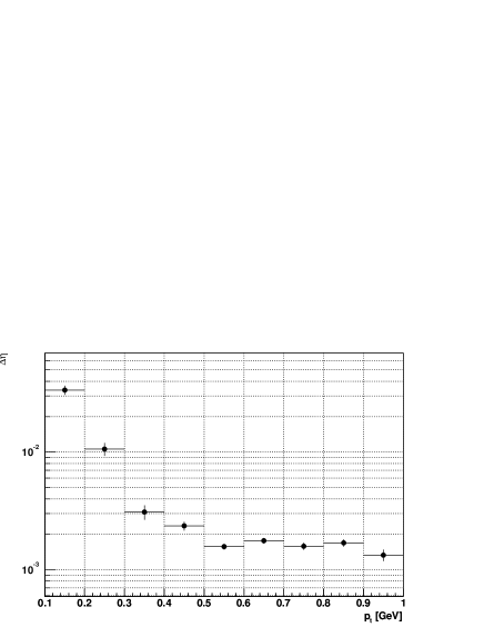
Figure 4.23: Average spread in pseudo-rapidity, $\Delta\eta$, of signals produced by a given particle as a function of $p_{t}$.

The spread is obtained from the $\eta$-distribution of the signals produced by a given particle. Such a plot thus gives an estimate of how much of the signal from a particle will be contained within a given $\eta$-sub-volume. $\Delta\eta$ increases below $p_{t}$ of 0.3-0.4 GeV, while for higher momentum the spread saturates at $\Delta\eta\sim$0.001-0.003. This observed increase at lower momentum is mainly due to the fact that particle energy loss and multiple scattering becomes more significant for lower momenta.

Based on the simulated spread, a uniform segmentation of $\eta$ with intervals of size 0.01 has been done. This leads to about 100 sub-volumes in the central cone of $|\eta|<$ 0.9.

Parameter space

The properties of the parameter space are determined by the choice of image space. In particular, the range of the histogram axis is defined by the possible values of the track parameters. The parameters consist of the curvature of the track, $\kappa$, and the emission angle with the $x$-axis, $\psi_{0}$. The curvature of the track is inversely proportional to the transverse momentum of the particle, Equation 4.1, and the maximum value of $\kappa$ is thus defined by the minimum value of $p_{t}$:

$$|\kappa|_{\mathrm{max}}=\frac{0.3B}{p_{t,\mathrm{min}}}.$$ (4.49)

In this context, $p_{t,\mathrm{min}}\$ corresponds to the lower limit of the desired $p_{t}$ range to be measured. Once the $\kappa$-range is defined, the range in $\psi_{0}$ can be given by taking the inverse of Equation 4.26,

$$|\psi_{0}|_{\mathrm{max}}=\phi_{m}-\sin^{-1}\left(\frac{r_{m}}{2}\kappa_{\mathrm{max}}\right),$$ (4.50)

where $(r_{m},\phi_{m})$ is the polar coordinates of a point on the line which confines the image space, Figure 4.24.

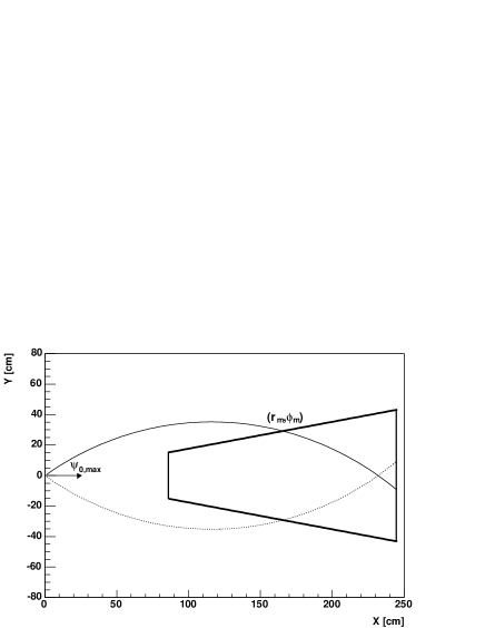
Figure 4.24: Parameterization of the HT image space. The parameter range of the HT parameter space is defined by the minimum $p_{t}$ (maximum curvature, $\kappa$) and a point $(r_{m},\phi_{m})$ on the line which confines the image space in the transversal direction (this line corresponds to the TPC sector boundary).

This line corresponds to the azimuthal angle of the boundary of the TPC sector. The point is chosen to be in the middle of the TPC barrel, in order to avoid an unequal distribution of the track segments in neighboring sectors.

The fact that the maximum values of $\kappa$ are defined by the minimum value of $p_{t}$, makes it possible to apply a lower $p_{t}$-cut in a straight-forward way. Particle tracks with a higher curvature than the range of the histogram axis will not create a valid peak in the parameter space, and will thus be excluded from the pattern recognition. This can be exploited by the algorithm, which can be optimized to search for tracks within a certain $p_{t}$-range.

The sampling intervals of the parameter space were chosen according to the average spread of the formed peaks in the simulations. The relative size of the intervals were selected in order to avoid possible under- or over-sampling, Equation 4.44.

4.6.3 Data flow

Similar to the sequential tracking code, the iterative reconstruction chain has been implemented in modules in order to be highly configurable with respect to different process topologies. Each processing step has however certain requirements with respect to locality and data flow.

HT The HT is a pure accumulation procedure, and consists of incrementing an array of counters for every input point. The algorithm is parallel by nature, since the transform of each image point is treated independently. However, the requirement on the image space with respect to the peak significance versus background makes it necessary to include a minimum number of data volume as input data.

Peak Finder Peak finding is done independently on each accumulator array. Each peak array may thus be processed in parallel.

Cluster Fitter The Cluster Fitter closely resembles the Cluster Finder as far as parallelization is concerned. They are both restricted to the two-dimensional pad-row-plane without any need of information from the other pad-rows. However, the Cluster Fitter requires the track parameters as input for the fitting procedure, and thus needs information on the tracks that crosses the pad-row being processed.

Figure 4.25: Data flow for the iterative reconstruction chain.

A possible data flow scheme is shown in Figure 4.25. In this scenario the HT is performed in parallel on each sub-sector, whereas the resulting accumulator arrays from each sub-sector within a sector are added according to Equation 4.48. The arrays are then processed by the peak finder, whose output is a list of track candidates. The list of tracks are passed to the Cluster Fitter (Section 4.6.1), which reconstructs the clusters along the helix trajectories. In order to obtain the optimal track parameters, the collected space points belonging to each track are fitted to a helix using the Track Fitter algorithm, Section 4.5.3.

4.6.4 Performance

The complete reconstruction chain, as outlined above, has been evaluated for different particle multiplicities. In order to compare the results with the results from the other tracking algorithms, the same definitions concerning tracking efficiency as described on page 4.5.6 have been used. The results are compared to both the sequential tracking scheme and the standard Offline chain, here referred to as HLT sequential and Offline, respectively.

Tracking efficiency

Figure 4.26 shows the tracking efficiency as a function of $p_{t}$ for two event samples of multiplicity dN_ch/d$\eta$ = 1000 and dN_ch/d$\eta$ = 4000, respectively. All primary particles with $p_{t}\geq$ 0.15 GeV were included in this evaluation, and the boundaries of the parameter space were adapted accordingly. At dN_ch/d$\eta$ = 1000 the efficiency is slightly lower than for both HLT sequential and Offline. In particular, the efficiency drops in the low momentum regime for $p_{t}$ $\leq$ 0.5 GeV. For higher $p_{t}$ the efficiencies shows similar behavior for all approaches. At higher multiplicity, dN_ch/d$\eta$ = 4000, the track efficiency in the iterative approach is significantly lower than both the HLT sequential and Offline reconstruction chain.

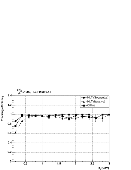
Figure 4.26: Tracking efficiencies as a function of $p_{t}$ for two multiplicity samples. All tracks with $p_{t}$ $\geq$ 0.15 GeV have been included in the evaluation.

In Table 4.4 the ratio between the number of track candidates found by the HT, and the number of tracks reconstructed by the Cluster Fitter are listed for the two event samples. This ratio provides an estimate of the relative number of false track candidates which originate from falsely identified peaks in the HT parameter space. The ratios indicate that more than 70% and 130% of all the track candidates from the HT failed to be reconstructed by the Cluster Fitter for the two multiplicities, respectively.

	Ratio
dNch/d$\eta$	$p_{t,\mathrm{min}}\geq$ 0.15 GeV	$p_{t,\mathrm{min}}\geq$ 0.5 GeV
1000	1.75	1.39
4000	2.35	1.32

Table 4.4: Ratio between track candidates found by the HT and tracks reconstructed by the Cluster Fitter.

The right column in Table 4.4 shows the corresponding ratios for the case where the parameter space in the HT has been restricted to only include tracks for $p_{t}$ $\geq$ 0.5 GeV. In this case the ratio decreased to $\sim$1.3 for both multiplicities, indicating that the major part of the fake track candidates originates from the lower $p_{t}$-range.

Figure 4.27 shows the tracking efficiencies for the same event samples as evaluated for the sequential track reconstruction chain, Figure 4.7. Due to the problem with fake tracks at lower momentum, the parameter space in the HT was optimized for tracks with $p_{t}$ $\geq$ 0.5 GeV, and consequently only particle tracks with $p_{t}$ $\geq$ 0.5 GeV were included in the evaluation. At lower multiplicities (dN_ch/d$\eta$ $\leq$ 2000) the tracking efficiency of all approaches are similar for this $p_{t}$-region. At dN_ch/d$\eta$ = 4000, however, the efficiency of the iterative approach is significantly lower than for the HLT sequential and Offline reconstruction chains.

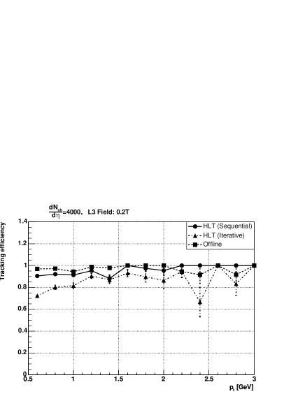
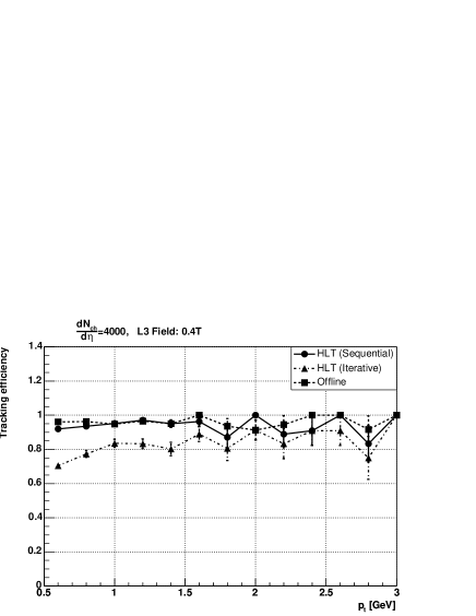
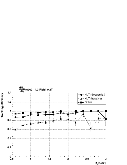
Figure 4.27: Tracking efficiencies as a function of $p_{t}$ for four different multiplicities at both magnetic field settings of 0.2T (left) and 0.4T (right). Only tracks with $p_{t}$ $\geq$ 0.5 GeV/c were included.

Momentum resolution

Figure 4.28 shows the transverse momentum resolution for two of the event samples in Figure 4.27. At the lower (dN_ch/d$\eta$ = 1000) multiplicity the iterative approach is slightly better than the sequential approach. At higher multiplicities (dN_ch/d$\eta$ = 4000), however, the iterative approach is lower than both sequential and Offline.

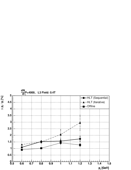
Figure 4.28: Transverse momentum resolution for two multiplicities. Only tracks with $p_{t}\geq$ 0.5 GeV were included.

Remarks on the tracking performance

The results indicate that the implemented iterative reconstruction chain has clear limitations when going to higher multiplicities. The main reason for this shortcoming is the relative high number of falsely identified track candidates from the HT. The subsequent Cluster Fitter has no way of distinguishing these false track candidates from the valid ones. As a consequence, the input to the fitting procedure of a given cluster distribution might be wrong, and the fit procedure fails. This effect becomes increasingly significant as the occupancy increases, which is demonstrated by the fact that both the tracking efficiency and transverse momentum resolution deteriorates at higher multiplicities.

The relatively high number of fake tracks is mainly due to the complexity of the formed structures in the parameter space. In general, the peak formation depends on both the location of the points on a track segment in space and the errors of the points. In addition, energy loss and multiple scattering will cause the trajectories to deviate from their circular pattern, which leads to an additional smearing of the peaks. All of these effects complicates the peak finding, since the structured backgrounds is difficult the distinguish from the real peak formations. As a consequence, the criteria for selecting a valid peak needs to be relaxed, and background formations will be wrongly identified as track candidates.

Computing requirements

The required processing time of the various steps of the HT has been measured on a standard PC of 800 MHz Twin Pentium III, 256 KB L2 cache, running a Linux kernel v2.4. Table 4.5 lists the CPU-time for a multiplicity of dN_ch/d$\eta$ = 4000. The measurements are resolved with respect to the different computing steps, and the values thus corresponds to the time needed by a single processing module when implemented according to the scheme shown in Figure 4.25. The HT needs about 3.5 s to process the data within a single sub-sector, resulting in a total HT processing time of 750 s for the complete event. It should be noted that the algorithm was already optimized by utilizing look-up tables for the accumulation procedure [51].

Process	Locality	CPU-time [s]
HT	Sub-sector	3.5
Histogram add	Sector	1.2
Peak finder	Sector	1.8

Table 4.5: Measured CPU-time for the different processing steps in the HT. The measurement was done for an event sample with multiplicity of dN_ch/d$\eta$ = 4000. The locality refers to where the respective process is running, according to the data flow shown in Figure 4.25.

The results clearly indicate that the HT is very CPU-inefficient. The reason is that the processing is particularly I/O-bound as is needs extensive and repetitive access to large accumulator arrays. Due to their relative large sizes and numbers, the memory requirements are too large to fit in the cache of the CPU, and thus the timing numbers will scale poorly with the CPU clock frequency. However, the inherit degree of locality and parallelism of the HT makes it suited for implementation in FPGA co-processors [51].

4.7 Summary

In this chapter two different approaches for pattern recognition in the ALICE TPC for the High Level Trigger system have been presented. The two approaches have both their advantages and limitations with respect to complexity, implementation and performance.

Sequential tracking has shown to be efficient for lower multiplicities, both with respect to the quality of the reconstructed tracks and the required processing time. The achieved tracking performance is at the same level as the Offline reconstruction chain for multiplicities dN_ch/d$\eta$ $\leq$ 2000. At higher multiplicities, the tracking efficiency drops, in particular in the low momentum regime. The reasons for this are well understood. It is evident that the straight forward Cluster Finder approach fails to reconstruct the cluster centroids once the occupancy is too high. This is due to its lacking capabilities of unfolding the overlapping charge distributions.

In the iterative approach, an attempt has been made to improve the cluster reconstruction by providing an estimate of the track parameters prior to a cluster fitting procedure. This was done by applying an implementation of the Hough Transform on the raw ADC-data. Here the located track candidates were used as an input for a two-dimensional cluster fitting and deconvolution of the overlapping clusters. The advantage of this approach is the simplicity and inherit degree of parallelization of the Hough Transform, which makes it an clear candidate to be implemented very early on the readout chain within the HLT system, possibly utilizing the FPGA co-processors planned for the HLT-RORC. However, the HT produces a very high number of false positives, which complicates the cluster fitting. As a result, the resulting tracking performance is less than that of the sequential approach.

Alternative solutions to improve the tracking efficiency for higher multiplicities are discussed in Chapter 6.

Chapter 5 TPC Data Compression

The option to compress the detector data efficiently enables a potential increase of the event rate to mass storage, even without performing event selection. All physics observables will benefit from such an application. Applicable data compression schemes and their expected performance on ALICE TPC data are presented in this chapter.

5.1 Introduction

The ultimate goal of data compression is to reduce the number of bits required to store information, without any significant information loss. From a information theory point of view, data compression techniques can be divided into two main categories; lossy and lossless. A lossy data compression does not guarantee a bit-by-bit reconstruction of the original data set, and may therefore concede a certain loss of accuracy. In exchange however they may provide a greatly increased compression factor. Lossy compression techniques are commonly applied to graphics and digitized sound, as the digitized representations of such analogue phenomena includes a certain degree of noise anyhow. Most lossy algorithms can be adjusted to different quality levels, gaining higher accuracy in exchange for less effective compression. Lossless compression techniques, on the other hand, guaranty that an exact duplicate of the input data stream is generated after a compress/expand cycle. These techniques are applied when the loss of even a single bit can affect the information content significantly.

In general data compression consists of taking a stream of symbols and transforming them into codes. If the compression is effective, the resulting stream of codes will be significantly smaller than the original data size. The decision to output a certain code for a certain symbol or data subset is based on a model. The model is a collection of data and rules to process the input data and determine which codes to output.

The most effective compression results can be achieved if the model is well adapted to the underlying data. A well-known example is the approach used by the MP3-format for audio files, where the results achieved when sound is compressed adapted to human hearing characteristics are much better than the results from general purpose algorithms. In case of TPC data the underlying data is the ADC-data, the clusters and tracks, while all the relevant information is contained in the final reconstructed physical observables. Before discussing the various compression algorithms applied, a brief summary of the characteristics of TPC data with respect to the various signal generation errors is given.

5.2 TPC signal generation and models

An effective data compression scheme has to be well adapted to the underlying data model and the noise already present in the data. As long as the allowed loss of accuracy does not exceed the inherit accuracy already present in the data, the compression scheme will in general not alter the information content. Prior to discussing applicable data compression techniques for TPC data, the understanding of the signal generation and the resulting inherit error sources within the original data stream is necessary.

Error sources within the TPC signal generation

The ultimate task of the TPC is to measure the kinematics of the traversing particles and contribute to the particle identification by energy loss measurement. Before the data is readout out from the detector, several factors contributes to alter the data. These can be summarized as follows:

• Elastic and inelastic scattering.
  Both prior to entering the sensitive volume of the TPC and within the gas of the TPC volume, the charged particles interact with the surrounding material, causing the particle track to deviate from its original trajectory. These effects include both elastic scattering from nuclei, and inelastic collisions with the atomic electrons of the material. The energy loss is described by the Bethe-Bloch formula, and typically follows a Landau distribution.

• Diffusion.
  The drifting electrons diffuse when drifting towards the end-caps of the TPC, and hence influence the position resolution of the reconstructed space points. The drifting cluster of electrons can be described by e.g. a 3D Gaussian distribution, where the widths are determined by the diffusion constants of the gas (see Section 4.3.2, page 4.6).

• Electron attachment.
  During the drift the electrons can be absorbed in the gas by formation of negative ions.

• Gas amplification.
  Each of the liberated electrons is subject to gas multiplication when entering the readout chamber. This amplification is described by a exponential probability distribution. The gas gain properties of the gas has also a strong dependence on the temperature.

• E$\times$B-effects.
  The fact that the E and B fields are not parallel near the anode wires, leads to a displacement of the drifting electrons when entering the readout chamber.

• Front-end electronics.
  When the image charge induced on the readout pads is processed through the front-end electronics several sources contribute to the noise and distortion of the original signal. Tail cancellation, pedestal subtraction and zero suppression are all lossy compression techniques in their manipulation of the original raw data.

• 10-to-8 bit compression.
  The ADC conversion gain is typically chosen so that $\sigma_{\mathrm{noise}}$ corresponds to 1 ADC count. This means that the relative accuracy increases with the ADC-values, and is not needed for the upper part of the dynamic range. The ADC-values can therefore be compressed non-linearly from 10 to 8 bits leading to a constant relative accuracy over the whole dynamic range (Figure 5.1). The conversion from 10 to 8 bit of the ADC-values is thus a data volume reduction with some information loss, but keeping the relative accuracy for the single ADC-value.

All of these effects modify the original data, preventing an exact event reconstruction. Therefore, the complete readout system must be considered in order to decide to which extend lossy or lossless data compression should be applied. Also, since the relevant information in the data lies in the final outcome of the analysis, any lossy compression should be evaluated from its impact on the reconstructed physics observables.

Local and global TPC data models

In the context of TPC data compression, the applicable compression techniques can be divided into two main categories; local and global modeling. Local modeling techniques are applied on the scale of raw ADC-data, i.e. after a compress/expand cycle the resulting data will still consist of the same ADC-data format. In the latter case the data is described within a more global model, the clusters and tracks. In such a compression scheme, the final uncompressed data may not consist of ADC-data, but rather cluster and track parameters themselves. The difference between these two approaches is obviously the elimination of the original raw data from the data stream. However, as the vital information in the TPC data is contained in the reconstructed particle trajectories, there is in principle no need to keep the raw ADC-data.

5.3 TPC data format and coding

TPC readout data format

The ALICE TPC raw data format which will be used during the running of the experiment is defined by the ALTRO chip in the TPC readout-electronics chain, Section 2.4.3. In addition to the digitization of the input signals, the ALTRO performs the zero-suppression of the digitized data. This is basically a data compression technique that consists of detecting the hits in the time-direction and discarding the noise in between by replacing it with zeros. It is implemented using a sequence detection scheme, which is based on the rejection of isolated samples with a value smaller than a threshold level. Both the thresholding and hit-finding are lossy data compression techniques, as small clusters or tails of the clusters might be discarded from the data.

The zero-suppression results in long sequences of zeros between the hits. Run-Length Encoding (RLE) subsequently compresses these zeros. The principle of RLE is to replace a sequence of identical symbols by a certain character or tag, and the length of the sequence. In case of the TPC the RLE is performed on the zeros. This is thus equivalent to storing only the hits and their positions. As the RLE does not modify or discard any data, it is a lossless data compression technique.

The ALTRO data format consists of a list of sequences written in a back-linked structure [35], where each sequence is described by three fields: Temporal information (temporal position of the last time-bin in the sequence), sequence length (number of time-bins in the sequence) and the ADC-values themselves.

Simulation and coding

Simulated data were generated within the AliROOT framework Section 4.3. All events were generated using the HIJING parameterization for different multiplicities, and the standard TPC slow simulator including the complete detector response simulation package. The output from the simulation thus correspond to zero-suppressed 10-bit ADC-data, whose format is defined within special AliROOT data containers. Before any of the data compression techniques presented in this chapter were applied, the data was further modified in three steps:

1. A 45-degree (relative to the beam axis) cone was cut out of the data in order to remove data from particles which are not in the geometrical acceptance of the outer detectors. This will be done also during readout of the TPC detector, as the low $p_{t}$ tracks crossing the TPC under small angles are too problematic to resolve. This cutout reduces the original data volume by $\sim$40%.

2. The simulated 10-bit ADC-data were transformed into 8-bit data by a 10-to-8 bit table shown in Figure 5.1.

3. The final 8-bit ADC-data were then RLE and written to binary files for subsequent comparison to the compressed data. The adapted data format uses a coding scheme whose size resemble the ALTRO-format. Further details about the format used can be found in Appendix B.2.

All compression ratios in the following are calculated as

$$\frac{\mathrm{Compressed\ size}}{\mathrm{Original\ size}}\times 100\hskip 14.22636pt[\%]$$

where the original size refers to the RLE 8 bit ADC-data.

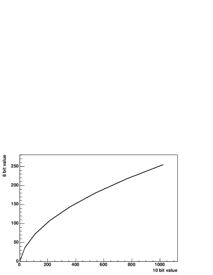
Figure 5.1: Plot of the 10-to-8 bit conversion table used [80].

5.4 Local modeling techniques

In [55] several data compression techniques, based on local data modeling, were applied on TPC data. Both data from the NA49 experiment, and simulated data from the ALICE TPC, were studied. A brief introduction to the different algorithms applied and the achieved result is given in the following.

5.4.1 Lossless TPC data compression

In general, most lossless compression techniques are based on entropy coding. Such algorithms exploit any possible redundancy within the information message, and the fact that the different symbols within a message are not equally probable. A symbol, which has a very high probability of occurrence, will be coded using very few bits, while symbols with a low probability are coded with a larger number of bits. For TPC data, such a scheme can exploit the fact that different ADC-samples are not equally probable: Small ADC-values occur more often than larger ones, Figure 5.2. The theoretical limit on the average word size that can be achieved with such a strategy is given by the entropy of the data source. For TPC data the entropy can be computed as

$$E=-\sum_{A\in\Omega}p(A)\log_{2}p(A).$$ (5.1)

Here $p(A)$ is the probability of having a ADC-value, $A$, in the data, and $\Omega$ is the set of all possible words that are contained in the data source. The difference between the number of bits used to represent a single character and its information entropy is the potential for entropy coding techniques.

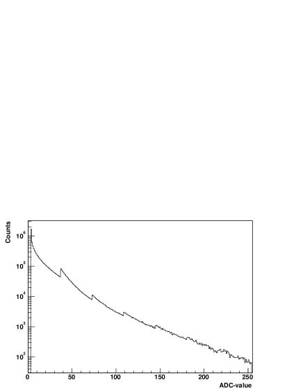
Figure 5.2: Distribution of ADC-values in simulated ALICE TPC-data.

Huffman Coding One of the most common entropy coding techniques is the Huffman Coding [81]. This algorithm has proved to be easily implemented and achieve good compression results without extensive processing power. The basic idea is to assign each input signal to a leaf of a binary tree, the so-called Huffman Tree. Each branch on this tree is either assigned the 0 or 1 bit, and the path from the root node to the leaf defines the code used for this symbol. By adapting the tree to the probability distribution within the data sample, symbols with higher probabilities get shorter codes and vice versa.

Arithmetic Coding A somewhat more complicated but potentially more effective compression technique is Arithmetic Coding. In contrast to Huffman coding, this approach does not produce a code for each symbol, but rather a code for an entire message. It is therefore not restricted to using integral number of bits per code, and is thus potentially more effective than the Huffman Coding. This compression technique can theoretically approach the lower limit given by the entropy [82]. The main idea is to assign to every symbol an interval between 0 and 1, with a size according to the occurrence probability of that symbol. For each input symbol the interval is shrunk to the range assigned to the new symbol. In this way the interval gets smaller and smaller and the input stream of symbols is replaced by a single floating point number representing the encoded message. The main drawback with Arithmetic Coding is that a relatively large number of operations are needed to encode a single symbol.

Differentiation A common approach for lossless graphics compression is differentiation, which exploits the fact that adjacent symbols may be similar. This is particularly true for TPC-data, where adjacent ADC-values are highly correlated. In this case the distribution of the derivative of the input has lower entropy than the data itself.

Code table coding A similar approach to differentiation is predictive encoding. In this case the next value in the data stream is guessed based on the previous sent value, and only the difference between the guess and the actual value is sent. Thus, if the guess is close to the actual value, the entropy of the difference is small.

5.4.2 Lossy TPC data compression

The best compression results can always be achieved if small noise-like changes of the data can be tolerated. The term lossy originates from the fact that these methods do not allow a bit-by-bit reconstruction of the original data set. Lossy compression techniques usually introduce some kind of quantization of the data, thereby lowering the required number of bits needed to store the information. In the simplest form, the data samples can be quantized into intervals corresponding to the required resolution.

Vector Quantization One of the more sophisticated quantization techniques is Vector Quantization [83]. Here statistical dependencies between successive data samples are exploited. Instead of quantizing data samples independently, several samples are grouped together to form a vector of data samples. In the TPC data, such a vector can typically be a sequence of ADC-values. The vector is compared to entries in a codebook of vectors, and the index of the best matching vector in the codebook is stored. In order to achieve effective compression factors the codebook has to be trained on the statistical properties of the data. Since such a codebook is pre-produced, only the given vectors are available to represent the data. Since this can lead to rather large quantization errors, also the difference between the input data and the selected codebook entry, the residuals, can be stored. These residuals can further be quantized and entropy encoded.

5.4.3 Results

The resulting compression factors obtained with the algorithms described above are summarized in Table 5.1. For the Huffman Coding, separate trees were built for the ADC-values and the header information, i.e. position and length. The Code table coding implemented a table that included a best guess for each combination of the preceding values. The results did not improve if the table was dependent on two of the preceding values. For the Vector Quantization it was shown that the impact on the physics observables is measurable but small, with the space point resolution being the most sensitive quantity.

Type of encoder	Entropy	Relative event size [%]
Zero suppressed raw event size	8	100
Arithmetic Coding	6.4	80
Code table coding	5.7	71
Huffman Coding	5.2	65
Vector Quantization	5.1-3.8	64-48

Table 5.1: Compression performance for local data modeling techniques on simulated ALICE TPC data [55]. The entropy is given as the average number of bits used to encode a sample. For the Vector Quantization the entropies depends on the treatment of the residuals.

5.5 Global modeling techniques

The standard compression techniques listed in Table 5.1 are all applied on the scale of ADC samples and sequences. However, the TPC data can be described within a more global model, the tracks and their corresponding clusters. Such models can be exploited by compression methods by using it to transform the data into an more efficient representation, and thereby reducing the redundancy information (entropy) in the input data. Instead of storing the TPC data on the ADC-level, the information can be stored on a higher extraction level such as cluster and track parameters. The main difference of such models from the local techniques is that they require some form of pattern recognition to be done prior to the compression scheme. In this context the purpose of the pattern recognition is different from the normal case since the aim is not to extract physics information about the particle kinematics, but to build a data model.

In general the TPC pattern recognition scheme is a two-folded process, which corresponds to reconstructing the space points from the clusters and combining the space points into tracks, Chapter 4. From this point of view, there are two levels in which TPC data can be represented:

• Space point data.

• Space point data relative to their tracks.

The first case corresponds to storing only the space points and their properties. Thus, only a cluster finding procedure needs to be done prior to the compression. In the latter case, it is assumed that a zeroth-order tracking step is performed in which the space points are encoded with respect to their distance to the tracks they belong to. Both of these methods will eliminate the original raw data from the data stream, as the final data set after decompression in either case will consist of a list of clusters.

5.5.1 Storing cluster data

The TPC clusters represent the three dimensional space points of the particle trajectories. The information which is needed from an analysis point of view consists of the three dimensional coordinates, the shape of the cluster and the total charge of the corresponding cluster. To first order each of these values would have to be stored with the required number of bits to ensure the information content. However, from the way the data is organized in the detector, some simplifications can be made.

The space points are reconstructed from the cluster centroids, which is calculated from the two-dimensional digitized charge distribution is the pad-row-plane. The coordinate in one dimension is thus given by the radius of the pad-row plane, and is consequently the same for all the clusters on the same pad-row. The remaining two coordinates can therefore be encoded with respect to the pad-row they are located on.

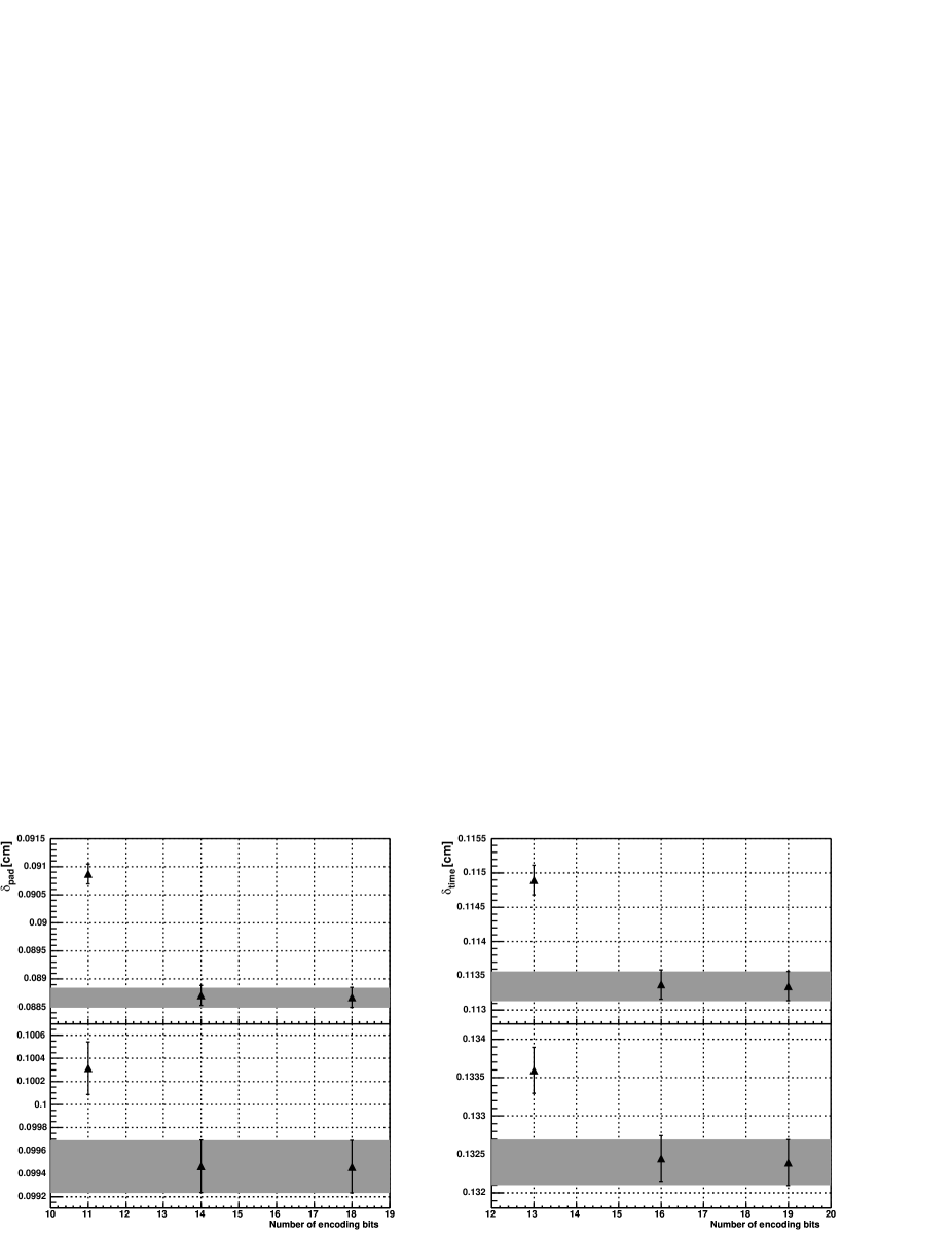
Figure 5.3: Space point resolution for different encoding sizes of the cluster centroids. The upper plots show the result for the outermost TPC chambers, while the inner plots shows the inner chambers. The shaded area shows the resolution within the original data set. The results were obtained by comparing the cluster centroids and the position of the corresponding simulated particle trajectory. The values correspond to the standard deviation from a Gauss fit.

The number of bits required to store the space point coordinates is determined by the inherit resolution within the data. The typical space point resolution of the ALICE TPC is at the order of 0.08 cm and 0.1 cm for the pad and time direction respectively. With a pad-width of 0.4 cm and 0.6 cm for the inner and outer TPC chambers respectively (Table 2.1), this corresponds to a precision of $\sim$0.1 in pad-coordinates. In order to avoid any deterioration of this resolution, this coordinate should thus be stored with at least 2 decimal precisions. Given that the maximum number of pads on a single pad-row is 140, a total number of 14 bits is needed to encode the pad-coordinate. Similar arguments hold for the time-direction whose absolute value can take up to 512 time-bins. With a 2 decimal precision this would then correspond to a spatial resolution of $\sim$0.006 cm and thus a total number of 16 bits for the encoding size.

Table 5.2 lists the number of bits required to

		Precision [cm]
Cluster centroid	Size (bits)	Inner	Outer
	11	0.04	0.06
Pad centroid	14	0.004	0.006
	18	0.0004	0.0006
	13	0.06
Time centroid	16	0.006
	19	0.0006

Table 5.2: Space point data and their required encoding size.

encode the positions using 1, 2 and 3 decimals for both pad and time direction together with their respective spatial resolutions. Figure 5.3 shows the impact on the space point resolution of keeping the respective levels of precision within the data. In the plots also the resolution within the original data, i.e. keeping the full floating point precision, is shown. As expected there is some impact on the resolution by keeping only a single decimal precision for both directions. No difference can however be seen when using 2 and 3 decimals. This indicates that the a total of 14 and 16 bits is needed to store the pad and time coordinate respectively without any information loss.

Cluster parameters	Size (Bit)
Pad coordinate	14
Time coordinate	16
$\sigma_{\mathrm{pad}}$	8
$\sigma_{\mathrm{time}}$	8
Total charge	12
Total	58

Raw-data parameters	Size (Bit)
ADC-values	3$\times$3$\times$8=72
Pad-numbers	3$\times$8=24
Time information	3$\times$32=96
Total	192

Table 5.3: Data parameters and their encoding size. Left table: Cluster parameters and the estimated number of bits required to store the respective parameters within the intrinsic resolution. Right table: Raw-data parameters and their estimated encoding size assuming a single isolated cluster of size 3$\times$3 bins.

In Table 5.3 the cluster parameters together with their required encoding size are listed. In addition to the two-dimensional centroid, also the cluster shape and the total charge are needed. In order to store the cluster widths with the same level of precision as for the centroids, each direction is encoded with 8 bits. The total cluster charge is stored using 12 bits. In total 58 bits are needed to store the complete cluster using this representation.

The above storage considerations can now be compared to the required size of storing the raw-data itself. However, the required encoding size for the raw-data depends in general on the size of the clusters in terms of number of bins in the pad-row-plane, and also on the multiplicity. For instance, assuming a single ’ideal’ cluster whose size is 3$\times$3 bins, a total of 3$\times$3$\times$8=72 bits are required to store the ADC-values. Furthermore, header information is needed to encode the position of the ADC-values in the pad-row-plane. This typically contains the respective pad-numbers on which the individual ADC-sequences are located and the relative time-information (Appendix B.2). Each pad-number can be encoded using 8 bits, thus 3$\times$8=24 additional bits are required for the 3 different pad-numbers. For the time-information 4$\times$8=32 bits are needed for encoding of zero-sequences and RLE tags. This results in a total of 192 bits, Table 5.3. Comparing with the encoding size for the cluster parameters, a reduction of about 70% may be achieved when storing the cluster parameters instead of the raw-data. This estimate however assumes that only one isolated cluster is present on a single pad-row, which of course in general is not the case. The relative size of the header information is strongly dependent on the occupancy, and will decrease as a function of multiplicity due to the fact that the sequences on a given pad are encoded according to their internal distance and the pad-number is stored only once per pad. This is illustrated in Figure 5.4 which shows the relative size of the cluster data for different multiplicities. Here, the HLT Cluster Finder algorithm was used to reconstruct the clusters, Section 4.5.1. For low multiplicities the ratio is $\sim$25%, while it increases to $\sim$30% for higher multiplicities. The fact that the ratio for very low multiplicity is $\sim$5% lower than the value estimated above, can be explained by the fact that the clusters are in general larger than the assumed 3$\times$3 bins.

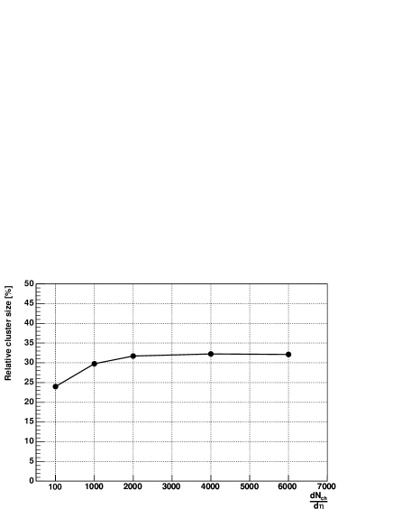
Figure 5.4: Ratio between cluster data and raw-data as a function of multiplicity. The cluster data was stored using the representation listed in Table 5.3.

5.5.2 Track and cluster modeling

Given the resolution of the space points and the size of the detector volume, the space points will lead to a rather large encoding size of the clusters. However, if the track reconstruction has been done the clusters are assigned to their respective tracks. Within this data model, the cluster positions can be encoded relative to the track parameters and thereby lowering the required number of bits needed to store the information.

The basic idea of this compression technique is to encode the data within the context of the reconstructed tracks and their corresponding clusters. Thus, the pattern recognition has to be solved prior to the data compression. Once the track reconstruction is completed, the tracks can be represented by helix parameters, and the clusters by their two-dimensional crossing point with the pad-row-plane. Let $(\Lambda_{\mathrm{pad}},\Lambda_{\mathrm{time}})$ denote a intersection between a track and the pad-row plane, and $(\lambda_{\mathrm{pad}},\lambda_{\mathrm{time}})$ the centroid of the corresponding cluster assigned to the track, Figure 5.5.

Figure 5.5: Definition of a residual. The residuals are defined as the distance, $\delta$, between the track crossing point, $\Lambda$, and the cluster centroid, $\lambda$, of the assigned clusters.

Further, let the distance between the track crossing point and cluster position, the residuals, be defined as

$$\delta_{\mathrm{pad}}=\Lambda_{\mathrm{pad}}-\lambda_{\mathrm{pad}},\hskip 28.45274pt\delta_{\mathrm{time}}=\Lambda_{\mathrm{time}}-\lambda_{\mathrm{time}}.$$ (5.2)

The residuals represent small deviations of the cluster position from the track model, and are subject to the intrinsic detector resolution. This offers the possibility to quantize the residuals with a transfer function whose resolution is adapted to the detector noise and resolution,

$$\delta_{\mathrm{pad}}\rightarrow\delta_{\mathrm{pad,Q}}=\frac{\delta_{\mathrm{pad}}}{\epsilon_{\mathrm{pad}}},\hskip 28.45274pt\delta_{\mathrm{time}}\rightarrow\delta_{\mathrm{time,Q}}=\frac{\delta_{\mathrm{time}}}{\epsilon_{\mathrm{time}}},$$ (5.3)

where $\epsilon$ is the respective quantization intervals chosen for the two directions. The resulting numbers can now be stored with a minimum number of bits required to encode the quantized residuals.

In addition to the cluster positions, also the cluster shape and total cluster charge is needed for the later offline analysis. As discussed in Section 2.4.1 the shape of a cluster is determined by the detector specific variables and the track inclination with the pad-row-plane. The cluster shape can thus be parameterized as a function of the track parameters, which allows the cluster shape to be restored without storing the actual shape. Optionally, the deviation of the cluster widths from the model can be stored.

Regarding the cluster charge, its value is determined by the number of primary collisions by the traversing particle in the gas which is a random variable described by a Poisson distribution. Due to secondary ionization and gas gain fluctuations the total charge is described by a Landau distribution with a long tail. Because of this, the representation of the cluster charge can not easily be reduced and is thus stored as the original value as calculated during cluster reconstruction.

Encoding scheme

A compression scheme which stores the track and cluster information in a compressed format has been implemented, and will be described in the following.

The input to the compression scheme are the reconstructed tracks and their corresponding assigned clusters. For every pad-row-plane the residuals are calculated and quantized according to Equations 5.2 and 5.3. The encoding scheme assumes the tracks have the following properties:

• The first and last point of the trajectory correspond to the innermost and outermost pad-row of the TPC respectively.

• A track may contain clusters from different TPC sectors.

In this scheme there is no need to store the pad-row number for every cluster, as the initial assumption is that there is a corresponding cluster on every successive pad-row throughout the TPC radius. Instead, only 1 bit is required to flag if this is not the case, i.e. to denote whether a cluster is present or not on a particular pad-row. Furthermore, an additional bit is also required to denote a possible change of the TPC sector. This may happen if the trajectory crosses the boundary between two neighboring TPC sectors.

A given data sample is encoded as illustrated in Figure 5.6.

Figure 5.6: Data compression encoding scheme.

Each track contains a bitmap which encodes the cluster presence. For every pad-row 1 bit is used to flag whether a cluster has been assigned or not on that pad-row. If no cluster is present, only the ’0’ bit is written, otherwise the cluster information is also stored. A second bitmap is used to store any change in TPC sector number. If a cluster in the list belongs to a different sector than the previous, this is stored by setting this bit to ’1’. In that case, the new sector number is stored in addition to the cluster information.

The compressed data sample consists of the track parameters of every track together with the coded cluster information for the corresponding clusters. The track parameters correspond to a minimum set of required parameters to describe a helix, Appendix A.2. These are the curvature of the circular motion, $\kappa$, the coordinates of the point at the distance of closest approach (DCAO), $(r_{\mathrm{DCAO}},\phi_{\mathrm{DCAO}},z_{\mathrm{DCAO}})$, and the dip-angle of the track, $\lambda$. In Table 5.4 these parameters are listed together with their respective encoding sizes. The size of the cluster parameters depends on the choice of quantization intervals, $\epsilon$, in Equation 5.3. The minimum number of bits required to store a quantized residual $\delta_{Q}$ is given by

$$n_{\mathrm{bits}}=\mathrm{max}[\frac{\log(|\delta_{Q}|)}{\log(2)}]+1\equiv n_{\mathrm{bits}}(\epsilon)$$ (5.4)

where max$[x]$ denotes the closest integer larger than $x$. The extra bit is needed to encode the sign. Thus for a given data sample the number of bits used to encode the residuals are calculated from the maximum value in the sample using Equation 5.4. The track–cluster parameters and their respective sizes are listed in Table 5.4.

Track parameters	Size (Byte)
$\kappa$	4 (float)
$\phi_{\mathrm{DCAO}}$	4 (float)
rDCAO	4 (float)
zDCAO	4 (float)
$\lambda$	4 (float)

Track–cluster parameters	Size (Bit)
Cluster presence	1
Sector / change	6 / 1
Cluster charge	12
$\delta_{\mathrm{pad,Q}}$	$n_{\mathrm{bits}}(\epsilon)$
$\delta_{\mathrm{time,Q}}$	$n_{\mathrm{bits}}(\epsilon)$

Table 5.4: Cluster and track parameters and their respective size used in the compression scheme. The track parameters are defined at the distance of closest approach to origin (DCAO). The number of bits used to encode the residuals is determined by the maximum value of the respective residuals in the sample, and are calculated from Equation 5.4.

Figure 5.7: Flow diagram of the implemented data compress/expand cycle.

The compress/expand cycle

In general, any implementation of a data compression scheme consists of two separate steps: compression and expansion. In the first step the given input data sample is encoded following the implemented encoding scheme. The compressed data sample can then be compared to the original in order to evaluate the compression ratio. Then, during the expansion, the compressed data sample is decompressed and restored into the same data format as the original data. Finally, the uncompressed data can be compared to the original data set in order to evaluate any impact on the relevant information content.

Figure 5.7 show a flow diagram of the complete compress/expand cycle which has been applied. In a first step the clusters and tracks are reconstructed from the 10 bit ADC-data. The resulting clusters and tracks are then encoded according to the scheme illustrated in Figure 5.6. The remaining clusters in the event which were not assigned to any tracks may optionally be written in addition to the compressed data, or they may be discarded all together. Alternatively a special selection of the remaining clusters can be done using a cluster analyzer (discussed on page 5.5.2). The data is then uncompressed by restoring the cluster centroids and shape from the compressed data, and optionally merging them with the remaining cluster data. The final list of clusters is then given to the offline track finder program. Once the tracks have been reconstructed, the resulting tracking performance can be evaluated in order to check the impact the compression has on the tracking performance. Furthermore, the compressed data size is compared to the original raw-data size, represented by the 8 bit ADC-data, to obtain the relative compression ratios.

On choosing the quantization intervals

The quantization interval, $\epsilon$, in Equation 5.3 determines the accuracy of the compression scheme. This is an essential parameter in the algorithm as it limits both the accuracy and the achievable compression factor of the algorithm. Selecting a very coarse quantization interval will in general allow for a greater compression factor as the number of bits required to encode the residuals will be small. Any such gain in compression factor will however come at the expense of a correspondingly lower space point resolution in the final uncompressed data sample.

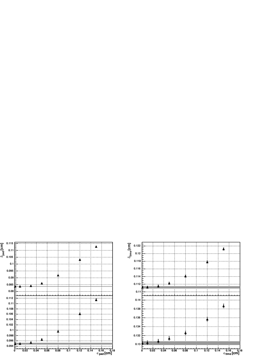
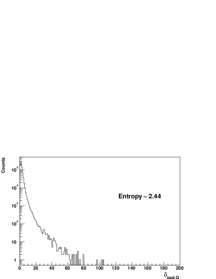
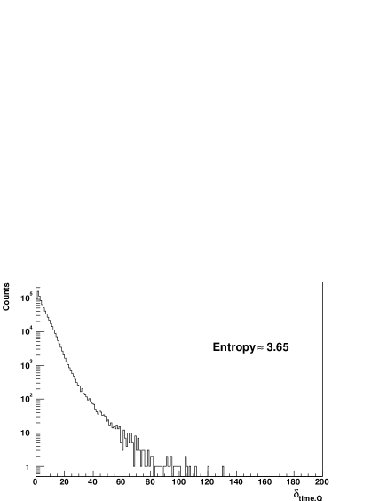
Figure 5.8: Impact of the quantization scheme on the space point resolution. The upper plots show the result for the outer TPC chambers, while the inner plots shows the inner chambers. The shaded area corresponds to the resolution within the original data sample. The resolutions were obtained from isolated clusters from all primary tracks with $p_{t}\geq$ 0.1 GeV. The values correspond to the standard deviation from a Gauss fit of the respective distributions.

Figure 5.9: Distribution of the quantized residuals for a quantization interval of $\epsilon$=0.05 cm. The data sample used are the same as used in Figure 5.9.

Figure 5.9 illustrates the impact of the quantization steps on the space point resolution. The plots show the final space point resolution after a compress/expand cycle as a function of the choice of quantization steps in the pad and time direction, respectively. The event sample correspond to a low multiplicity event (dN_ch/d$\eta$ = 100), i.e. well separated clusters and tracks, and the events were reconstructed by the HLT sequential track reconstruction chain, Section 4.5. As one would expect the space point resolution deteriorates as the quantization intervals increases. For $\epsilon$=0.05 cm, the loss is about 2% and 1% for the pad and time direction, respectively.

Figure 5.9 shows the distribution of the quantized residuals for $\epsilon$=0.05 cm. The distributions are approximately exponential. The maximum value of the distributions are 104 and 130 for the pad and time distribution respectively, which according to Equation 5.4 means that 8 and 9 bits are required to encode the residuals with a fixed bit-rate. However, given that values are not equally probable, further compression is possible by entropy coding. The entropy of the samples has been calculated according to Equation 5.1, and suggest a theoretical lower limit on the average word size needed to encode these residuals of 2.4 and 3.6 for the pad and time direction respectively.

Cluster widths

In addition to the cluster centroids, also the space point errors are needed for the track reconstruction. For the track finding algorithms, these errors are for practical purposes calculated from the cluster widths using suitable proportional factors optimized from the simulated data, Section 4.5.1. As the cluster widths can be parameterized according to the track parameters (Equation 4.17), this can be exploited by the compression scheme by removing the cluster shape information from the data stream and restoring it from parameterization during the decompression step.

However, since the cluster generation in the TPC is a result of stochastic processes, the cluster shape and also the space point errors are subject to fluctuations. As a consequence, the parameterization of the cluster shape may lead to deviations of the space point errors from the “true” errors. This can furthermore be a potential source for loss in tracking performance as e.g. the track reconstruction algorithm may make wrong decisions based on $\chi^{2}$-criteria if the provided error estimates differ significantly from the true ones. Such loss would in particular be expected to occur if the occupancy is large, in which the space point assignment critically depends on a good estimate of the individual space point errors.

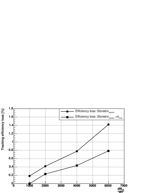
Figure 5.10: Integrated tracking efficiency loss due to removing the cluster shape information from the data stream ($\sigma_{\mathrm{param}}$). Instead of storing the cluster widths for each cluster, the widths are parameterized by Equation 4.17. The efficiency loss when the original cluster widths are stored for clusters where the measured widths deviate substantially from the parameterized ones are also shown, Equation 5.5 ($\sigma_{\mathrm{param}}+\sigma_{\mathrm{true}}$).

Figure 5.10 shows the loss in tracking efficiency due to removing the cluster shape information from the data stream as a function of multiplicity. In this case clusters reconstructed by the Offline cluster finder was used as input in order to avoid any effects resulting from difference in performance between the HLT and Offline cluster finder algorithms. The loss was estimated by taking the difference between the integrated Offline tracking efficiency in the case where the cluster shape was parameterized according to the track parameters and the original data set in which the cluster shape was stored. The results indicate that the loss increases slightly as a function of multiplicity, and reaches the maximum of $\sim$1.4% for dN_ch/d$\eta$ = 6000.

In order to minimize such a loss, the original shape information can be kept by storing the deviation of the parameterized widths from the true ones. Alternatively, the widths can be stored only for clusters whose widths differs from the parameterization more than a certain threshold value. The scenario is also shown in Figure 5.10. In this case the cluster widths has been stored for clusters where

$$|\sigma_{\mathrm{param}}-\sigma_{\mathrm{true}}|>\frac{1}{2}\sigma_{\mathrm{true}}.$$ (5.5)

This selection criteria includes $\sim$10-15% of all the clusters in the samples, and results in no observable efficiency loss at dN_ch/d$\eta$ = 1000. However, at higher multiplicities, dN_ch/d$\eta$ = 6000, a efficiency loss of $\sim$0.8% is observed.

The results indicates that the Offline track finder algorithm is rather sensitive to the estimation of the cluster shape. This may be explained by the fact that the Offline track finder has been highly tuned to the space point errors obtained from the simulated cluster shape [84]. In order to further optimize the compression scheme in terms of cluster shape and space point resolutions, a detailed understanding of the TPC response and the impact on the final Offline reconstruction chain is needed. Such a study can however only be done using real TPC data, as these data will contain other effects as well. The results presented in the following are obtained using only a parameterization of the cluster widths.

Remaining clusters

After the track finding procedure, a certain amount of remaining clusters will be present. These are clusters which were not assigned to any tracks during the track reconstruction procedure. The are several possible sources of these clusters, and they depend foremost on the efficiency of the track finding algorithm at hand. In general the most common source is particles with a very low $p_{t}$ whose tracks could not be reconstructed due to large multiple scattering and energy loss. This is in particular true for the so-called $\delta$-electrons, which are produced when particles transfer a relatively large amount of their energy into a single electron when traversing through the gas. The typical signal from such particles forms a large continuous cluster area because of their large inclination with the pad-row-plane. Since these particles are in general not of any interest, they will not be included in any Offline analysis and can therefore be considered as noise. Thus from a data compression point of view, such clusters should be removed from the data stream as they do not contain any relevant information.

The list of remaining clusters may however also include clusters that are not originating from “noise” particle tracks, but are merely a result of an inefficient track reconstruction chain. In order to minimize any loss of accuracy and efficiency in the output data, the remaining clusters may be written in addition to the compressed data. These clusters can however not be encoded with respect to any track model, and thus needs to be stored with the cluster parameters as proposed in Table 5.3. This will then contribute with an additional overhead to the compressed data size. On the other hand, if they are completely disregarded from the data, vital information may be lost as the list may contain “valid” clusters which were not assigned to any tracks by the track reconstruction algorithm. Such a loss can be significant if the tracking performance of the applied tracking algorithm is lower than the one that will be used for the later offline analysis.

An option to store the remaining clusters, or a certain selection of them, has been included in the compression scheme (Figure 5.7). Here, a cluster analyzer can classify clusters based on a selection scheme, and only store a fraction of the cluster list. The analyzer selects remaining clusters located within the detector region being used for the seed-finding procedure in the Offline track finder algorithm, Section 4.3.3.

The impact on the tracking efficiency from removing the remaining clusters is illustrated for a given data sample in Figure 5.11.

Figure 5.11: Impact on tracking efficiency from disregarding the remaining clusters in the compression scheme. The data sample corresponds to an event with multiplicity of dN_ch/d$\eta$ = 1000. The plots show the tracking efficiency as a function of $p_{t}$ before (original) and after (compressed) the compress/expand cycle has been applied. Left: All remaining clusters are removed from the data stream. Right: Only remaining clusters which are located in the region where track seed-finding is performed are stored.

The two plots display the Offline tracking efficiency as a function of $p_{t}$ both before and after a compress/expand cycle. In both cases, the input clusters and tracks to the compression scheme were reconstructed by the HLT sequential track reconstruction chain, Section 4.5. In the left plot, all the remaining clusters have been removed from the data sample. A significant loss of tracking performance is observed, resulting in an integrated loss of about 16%. In the right plot, the cluster analyzer was applied to the remaining clusters in which the resulting selection were stored while the rest is removed. In this case, the integrated efficiency loss is reduced to about 1.5%.

5.5.3 Results

In order to investigate the performance of the compression scheme outlined in the previous sections, the compress/expand cycle was applied to various simulated data samples. The input to the compression scheme presented in the following are clusters and tracks which were reconstructed using the implemented HLT sequential tracking approach presented in Section 4.5. All tracking performance results and impact thereon refer to the standard Offline track finder.

Impact on the momentum and dip-angle resolution

One of the observables, which should be sensitive to the compression, is the momentum resolution. According to Equation 4.3 the relative transverse momentum resolution depends on both the space point resolution and the number of space points assigned to the track. In Figure 5.12 the impact on the relative momentum resolution is shown for an event with multiplicity dN_ch/d$\eta$ = 1000.

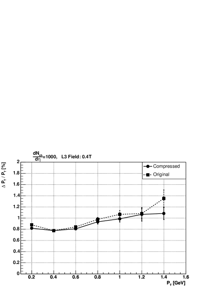
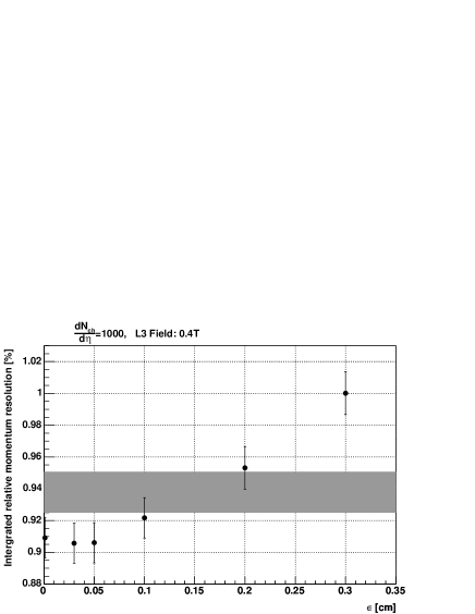
Figure 5.12: Impact on the relative momentum resolution from the compression. Left: Relative momentum resolution as a function of $p_{t}$ for both original data set and the compressed data sample. In the compression scheme the quantization intervals were $\epsilon$=0.05 cm. Right: Integrated relative momentum resolution as a function of the quantization intervals in the compression scheme. The shaded area corresponds to the resolution within the original data set.

In the left plot the resolution is shown as a function of $p_{t}$ for a quantization interval of $\epsilon$=0.05 cm for both the original and the compressed data sample. In the compression the remaining clusters selected by the cluster analyzer (Figure 5.11) were stored in addition to the compressed data. The plot indicates a slight improvement of the momentum resolution in the compressed data compared to the original for all $p_{t}$ -bins shown. In the right plot the integrated resolution is shown as a function of the quantization intervals used. For $\epsilon\leq$ 0.1 cm the momentum resolution is $\sim$3% better relative to the original data.

     

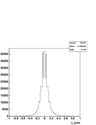
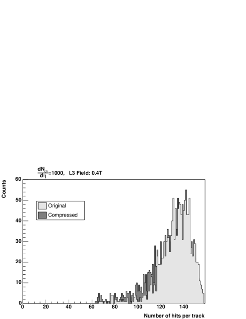
Figure 5.13: Transverse residual distribution before and after data compression. Left: Transverse residual distribution within the original data set. Right: Transverse residual distribution in the post-compression data set. The distribution has been obtained from clusters in the outer TPC chambers, and is averaged over all tracks in the event sample (dN_ch/d$\eta$ = 1000). Note the steps in the distribution which is due to the quantization.

Figure 5.14: Impact on the number of assigned clusters per track from the compression. The distributions corresponds to the number of assigned clusters per track before (original) and after (compressed) data compression has been applied.

The improvement in the resolution is an effect of the quantization of the residuals. As a consequence of this quantization, the resulting residual distributions are slightly narrowed as the residuals which are below the quantization interval are mapped to zero. This narrowing is illustrated in Figure 5.14. Here the transverse residual distribution before and after the applied compression scheme is presented, showing that the width of the distribution (represented by the RMS-value) is smaller for the post-compression distribution compared to the original data set. This effect leads to a better fit in the post-compression track finding and thus a more precise estimate of the curvature and correspondingly the momentum resolution. Furthermore, the potential loss of clusters will have a less significant impact on the momentum resolution as the number of space points has a 1/$\sqrt{\mathrm{N}}$ dependence compared to the linear dependence on the space point resolution. Figure 5.14 shows the number of clusters per track before and after the compression. A slight shift towards smaller values is observed for the compressed data sample. The mean value of the distribution changes by less than two clusters per track for the quantization intervals investigated.

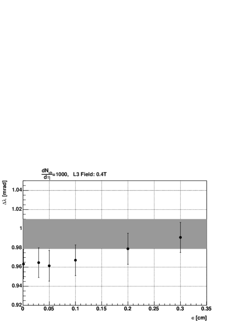
Figure 5.15: Integrated track dip-angle resolution, $\Delta\lambda$, as a function of the quantization intervals in the compression scheme.

Similar improvement of resolution can also be seen for the longitudinal part of the reconstructed tracks, which is illustrated by the impact on dip-angle resolution in Figure 5.15. Also here the resolution is shown as a function of the quantization intervals which have been used during the compression scheme. For $\epsilon\leq$ 0.1 cm the resolution is $\sim$4% better than within the original data.

Compression ratios versus tracking performance

In Figure 5.16 the achieved compression ratios are shown together with the corresponding loss in efficiency for 5 different multiplicities, with dN_ch/d$\eta$ ranging from 100 to 6000. The quantization intervals was set to $\epsilon$=0.05 cm for both pad and time direction. For every data set the compress/expand cycle was applied using three different options:

• Keeping all the remaining clusters.

• Keeping a selection of remaining clusters.

• Disregarding all the remaining clusters.

The second option applies the selection option discussed above which includes the clusters located in the region being used for seed-finding by the Offline track finder. The compression results are also summarized in Table 5.5.

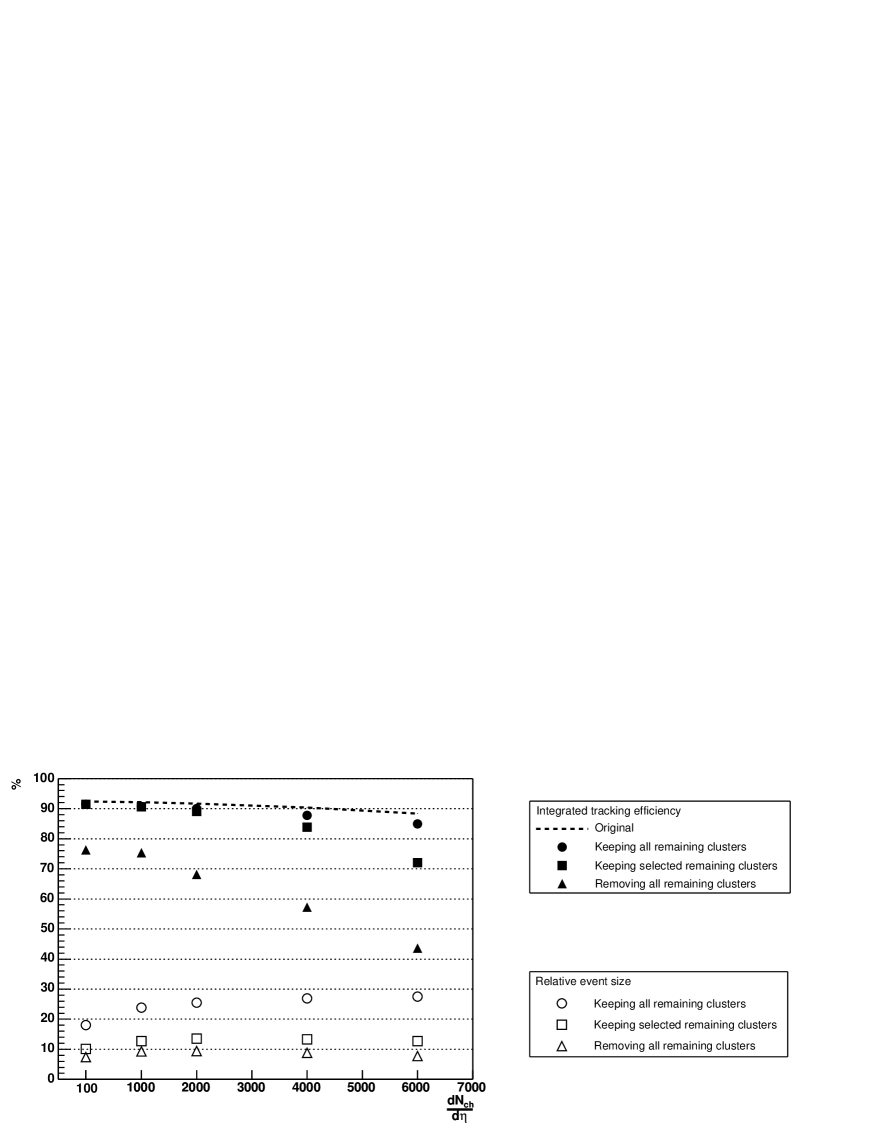
Figure 5.16: Achieved compression ratios and the corresponding efficiency loss for the different event samples investigated.

	Relative event size [%]
dNch/d$\eta$	All remaining	Selected remaining	No remaining
100	18.0	10.1	7.3
1000	23.8	12.7	9.3
2000	25.4	13.5	9.3
4000	26.9	13.3	8.8
6000	27.5	12.8	7.7

Table 5.5: Data compression ratios for the different event samples investigated. The three columns correspond to the various options of storing the remaining clusters.

It is generally observed that both the efficiency loss and the relative event size increases as a function of multiplicity. If all remaining clusters are kept in the data stream the resulting compression ratios range from 18-28%. In this case, a very small loss in efficiency can be observed for all the event samples with a maximum of 3.5% for dN_ch/d$\eta$ = 6000. In the case where only a selection of remaining clusters is stored, compression ratios of 10-14% are achieved. In this case, however, some loss of tracking efficiency can be seen, particularly for the higher multiplicity events. For dN_ch/d$\eta$ = 1000 the loss is on average $\sim$1.5%, while for dN_ch/d$\eta$ = 6000 it goes up to $\sim$16%. The third scenario, which disregards all remaining clusters in the data stream, indicates a significant impact for all the data samples investigated. In this case, the efficiency loss is on average $\geq$16% even for the lowest multiplicity of dN_ch/d$\eta$ = 100.

The observed loss in tracking efficiency is mainly caused by the shortcomings of the track reconstruction chain used to model the data, and not the compression scheme itself. This is also supported by the fact that the loss is insignificant at lower multiplicities, both with respect to the tracking efficiency and the impact on resolutions. For higher multiplicities, the applied tracking scheme has clear limitations compared to the approach used by Offline, which was demonstrated in Section 4.5.6.

In Table 5.6 the properties of the compressed data samples are listed.

	Bits used		Entropy		Relative size [%]
dNch/d$\eta$	Pad	Time	Pad	Time	Track parameters	Cluster parameters
100	7	8	2.4	3.6	6.0	94.0
1000	9	9	2.7	3.9	5.9	94.1
2000	8	9	2.7	3.9	6.6	93.4
4000	9	9	2.9	4.1	6.9	93.1
6000	9	9	3.0	4.3	7.3	92.7

Table 5.6: Properties of the compressed data samples. The bits used refer to the fixed bit-rate used to encode the residuals, while the entropy is the calculated entropy of the respective quantized residual distribution in the sample. The relative size gives the relative size of the track and cluster data in the compressed format.

In particular, the difference between the fixed bit-rate used to encode the residuals and their entropies indicate that the samples can be compressed even further by e.g. Arithmetic Coding. By simply taking the ratio between the calculated entropies and the number of bits used, an additional factor of 2-3 is achieved. The potential gain in the total compression ratio will however be slightly less than this factor, as the compressed data also contain the cluster charges, header information and the track parameters (Figure 5.6) which are difficult to compress any further.

5.6 Summary

In this chapter various options for compressing the TPC data as an application for the High Level Trigger System are presented.

Extensive studies applying local data modeling techniques on both real NA49 TPC data and simulated ALICE TPC data are published in [55]. The results show that lossless compression techniques such as Huffman and Arithmetic Coding can achieve compression ratios of $\geq$60%. The lossy Vector Quantizer may achieve ratios of $\sim$50% with a measurable, but small, impact on the space point resolution.

By introducing online pattern recognition, the TPC data can be modeled more efficiently by representing the data using cluster and track information. A data compression scheme which utilize the redundant information content by representing the cluster data relative to the track model has been implemented. Such a scheme will lower the bit-rate needed to encode the cluster parameters as the cluster model critically depends on the track parameters. Additional options to compensate for the potential loss of clusters in the compression scheme have been implemented in the cluster analyzer. These options include clusters that should be stored in addition to the compressed data sample. The results using simulated ALICE TPC data indicate that compression ratios of 10-15% are achievable. Even lower compressing ratios are possible by utilizing the entropy factor of the cluster residuals, e.g. using Arithmetic Coding. The entropies of the data samples indicate an additional compression factor of 2, depending on the overhead from the remaining clusters.

The relative loss in tracking efficiency is small for dN_ch/d$\eta$ $\leq$ 2000, and increases for higher multiplicities. The impact on the relative $p_{t}$ resolution and dip-angle resolutions was shown to be insignificant. The efficiency loss at higher multiplicities is solely due to the inefficiency of the HLT reconstruction chain and not the compression scheme itself.

Chapter 6 Conclusions and Outlook

In summary, two main topics are addressed in this work:

• Online TPC pattern recognition.

• Online TPC data compression.

The pattern recognition forms the basis of the HLT system as all the foreseen applications, both event selection and efficient data compression, relies on a full or partial online event reconstruction. The latter may be considered as the ultimate HLT-application as an effective online compression of the TPC data would potentially enable higher statistics for all the physics observables.

6.1 Online TPC pattern recognition

The critical performance issue both in terms of tracking efficiencies and computing requirements is the particle multiplicity. Present predictions for the multiplicity in central Pb–Pb collisions at LHC range from 2000 to 6000 charged particles per unit rapidity, and extrapolations from RHIC suggesting multiplicity values of about 2000-3000.

Tracking performance

Figure 6.1 shows the integrated tracking efficiency of primary particles as a function of multiplicity obtained with the HLT sequential tracking scheme. Two theoretical predictions, dN_ch/d$\eta$ $\approx$ 2200 [15] and dN_ch/d$\eta$ $\approx$ 3200 [16], are marked with the shaded area. Within this multiplicity range, the simulations indicate that tracking efficiencies of 85–90% are feasible.

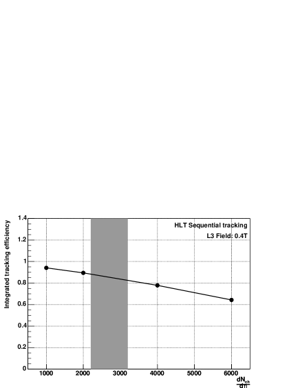
Figure 6.1: Integrated tracking efficiency obtained with the HLT sequential tracking approach. The shaded area indicates the present theoretical predictions based on extrapolations from RHIC [15, 16].

For the secondary particles, simulations indicate that more than 60% of the decay products from $K$ and $\Lambda$ particles within the TPC acceptance can be reconstructed with the current tracking scheme. With further optimizations of the tracking parameters this number is likely to improve.

At these relatively low multiplicities the resulting occupancy might be handled satisfactory by the implemented sequential tracking scheme. For higher multiplicities it is obvious that an iterative tracking approach is required in order to achieve the desired online tracking efficiencies. The implemented algorithms, the Hough Transform and a Cluster Fitter, however do not show any improved performance compared to the sequential chain. The main reason being the relatively high number of falsely identified peaks in the HT.

Impact on physics cases

The performance of the online track reconstruction algorithms must eventually be evaluated with respect to the impact on the various trigger applications. Such evaluation can only be done by extensive studies using the reconstructed tracks as input to the trigger algorithms. Some preliminary conclusion may however be drawn based on the current outlined trigger algorithms.

Most of the physics trigger applications such as the jet and open charm trigger relies on a good tracking efficiency for high transverse momentum particles. The jet trigger will mainly focus on particles with $p_{t}\geq$ 2 GeV, and the open charm trigger will utilize a online momentum filter where only tracks with $p_{t}\sim$ 0.5–1 GeV will be included in the search for $D$-candidates. In this region the tracking efficiency of the sequential approach is comparable to Offline for all multiplicities, as the relative efficiency loss is mainly restricted to lower momentum particle tracks. Also the iterative tracking approach shows promising performance in this momentum regime. This suggest that both tracking approaches may be utilized in such trigger applications. Further refinement of the open charm trigger in terms of secondary vertex analysis can only be done by including information by the ITS detector.

Suggestions for further work

Based on the current understanding of the ALICE TPC tracking performance, there are several optimizations and alternative solutions that should be pursued.

The fact that the sequential tracking scheme demonstrates a good performance at lower occupancies suggests the possibility of using it also for higher multiplicities in regions where the occupancy is sufficiently low, i.e. at large TPC radius. Reconstruction the tracks in the outermost pad-rows of the TPC with the Cluster Finder and Track Finder, these track segments can be extended towards the inner pad-rows by utilizing the Cluster Fitter. In such a scenario, the tracks reconstructed by the sequential tracking scheme serve as input to the Cluster Fitter where the charge distributions along the trajectory at the inner pad-rows are fitted and deconvoluted in order to properly reconstruct and collect the cluster centroids. The final list of assigned clusters may then be fitted to a helix in order to obtain the track parameters. Since the occupancy is low, the tracking parameters of the Track Finder should be relaxed in order to recover as many of the tracks as possible.

The cluster fitting procedure may also be further optimized. One option is to compare the estimated width of the cluster to be fitted to the calculated RMS-value of the actual charge distribution. Such a comparison can be used to determine the validity of the input track, and in particular reject input tracks whose estimated widths deviate substantially from that of the charge distribution. This may consequently reduce the number of fake tracks in the fitting procedure. Furthermore, global information about a track may be utilized in order to reject fake tracks at an early stage in the cluster fitting. For instance, a simple check may be performed on the input track on whether it points to valid clusters on a certain number of successive pad-rows. If the track is valid, there should be corresponding charge distributions along its trajectory on all the pad-rows.

Final optimization and tuning of the cluster fitting procedure can only be obtained using real ALICE TPC data, as a detailed understanding of the TPC response functions is needed to optimize the parameterization of the cluster shapes.

Computing requirements

The required computing power of the HLT system is directly influenced by the CPU-time needed by the individual processing modules in the event reconstruction chain. The largest amount of computing is by far required by the track reconstruction in the TPC, and the measured processing times of the TPC reconstruction chain may serve as a indicator on the amount of processing power needed for the complete system. Such estimates will however ignore any overhead from the interprocess communication and synchronization in order to operate the HLT system, and can only be indicative.

Given the rapid rate of increasing CPU performance, the number of single processors at the time of purchasing the HLT components will scale down relative to current available CPU performance. According to Moore’s law the processing power of a single processor will approximately double for every 18-24 months. Such a scaling is however restricted to applications which have a very low memory access requirements, i.e. it is only approximately applicable if all the data and code references are in the internal memory-cache of the CPU. This means that if an algorithm is heavily I/O bound, its processing time will not scale accordingly.

Table 6.1 lists the CPU-time measured on two different CPUs for the sequential reconstruction chain. The benchmark CPUs consist of Pentium III 800 MHz and Pentium 4 2800 MHz, both with 1 GB of RAM and 256 kB and 512 kB L2 cache respectively. Both architectures were running a Linux kernel v2.4. The measured CPU-time is integrated over all the processing modules, and is thus equivalent to the processing time needed to reconstruct one event on a single CPU. Based on these numbers one can estimate the required number of processors needed to process the data within the time-budget of 5 ms in central Pb–Pb rate of 200 Hz. For instance, assuming a multiplicity of dN_ch/d$\eta$ = 2000, about 6300 ms/5 ms=1260 CPUs (Pentium 4) is required to reconstruct the tracks in the TPC, while approximately the double amount is needed for dN_ch/d$\eta$ = 4000. Comparing the performance on the two processor types there is a factor of about 2.2 improvement in processing time, which illustrates that the processing times does not scale with the CPU clock frequency (3.5).

The Cluster Finder algorithm needs approximately 25% of the measured CPU-time. This algorithm has been synthesized on a FPGA, and will most likely utilize the FPGA co-processor functionality planned for the HLT-RORC. Assuming that the Cluster Finder can be processed in a single FEP, this can potentially reduce the number of required processors by a factor 4.

Given that the HLT components will be purchased in 2006-2007, an additional factor of increase of the CPU performance can be expected compared with todays measurements. How much this will affect the overall requirements of the HLT system, however, has to be monitored and evaluated during the purchasing procedure.

	Pentium III, 800 MHz		Pentium 4, 2800 MHz
dNch/d$\eta$	CPU-time [s]	#CPU	CPU-time [s]	#CPU
1000	7.5	1500	3.4	680
2000	14.0	2800	6.3	1260
4000	29.5	5900	13.2	2650
6000	47.3	9460	21.2	4240

Table 6.1: Computational demands on the HLT system from TPC tracking. The CPU-time is integrated over all the processing modules in the sequential tracking approach, and is equivalent to the processing time needed to reconstruct the event on a single CPU. The number of processors corresponds to the measured CPU-time divided by the available time-budget of 5 ms assuming event rate of 200 Hz.

6.2 Online data compression

The modeling techniques implemented indicate that one can compress the TPC data by a factor 6-10 with a low impact on the tracking performance. This however assumes that the online pattern recognition scheme which are used to model the data is comparable to that of which will be used during the Offline analysis.

Based on the achieved compression ratios one can estimate the potential online data rate reduction as far as the TPC is concerned. In Table 6.2, the event sizes estimated from RLE 8 bit ADC data and the corresponding data rate assuming a central event rate of 200 Hz are shown. These event sizes are scaled down using the compression ratios obtained and the resulting data rate is given accordingly.

	RLE 8 bit TPC data		Compressed track–cluster data
dNch/d$\eta$	Event size [MB]	Data rate [MB/s]	Event size [MB]	Data rate[MB/s]
1000	13.8	2760	1.8	360
2000	24.1	4820	3.3	660
4000	44.1	8820	5.9	1180
6000	61.6	12320	7.8	1560

Table 6.2: Estimated TPC data rate reduction based on obtained TPC data compression ratios. The compression ratios used corresponds to the results where a selection of the remaining clusters has been stored.

Given the foreseen bandwidth to mass storage of $\sim$1200 MB/s, the results indicates that up to a multiplicity of dN_ch/d$\eta$=4000 the data rate can sufficiently be reduced to write all the measured data to mass storage.

Entropy encoding of the quantized residuals by e.g. Arithmetic Coding may further improve the compression ratio by a factor of 2. However, also clusters belonging to secondary tracks must be considered, resulting in an increase of the compressed data size. With a good tracking efficiency they can be modeled and compressed similarly to what is done for the primaries. Including data from these tracks is not likely to have a significant impact on the compression ration, as their relative size is small. Their presence will therefore mainly concern the additional computing power needed for their reconstruction.

The difference between the modeling scheme, the general readout scheme and/or using e.g. entropy coding, is the elimination of the original raw-data from the data stream. However, the raw-data itself contains a significant amount of redundant information as its characteristics are governed by the detector specific constants such as the diffusion constants of the gas, electronic response functions etc. Therefore, once the Offline reconstruction and analysis chain has been set up correctly and fully understood, there will in principle be no reason to return to the raw-data anymore. During the first years of running the experiment, however, zero-suppressed raw-data will have to be recorded without any further processing in order to ensure a complete understanding of the TPC detector response. Any data compression scheme exploiting the global characteristics of the data is therefore likely not to be used during these first years of operation.

6.3 Outlook

Although recent results from RHIC indicate a particle multiplicity which is well below the original ALICE design value of dN_ch/dy=8000, the uncertainties are still very large. More effort should therefore be invested in further optimizing the algorithms for the higher multiplicity regime, possibly utilizing alternative combined tracking approaches as outlined above. Extensive studies are also needed to investigate the impact of the tracking performance on the various trigger applications, and adapt the tracking parameters accordingly. Furthermore, the other detectors, in particular the ITS and TRD, need to be incorporated into the HLT track reconstruction framework in order to enable full event reconstruction functionality. An obvious approach would be to implement an online version of the Kalman filter as used within the Offline framework.

Further optimization of the TPC data modeling and compression scheme relies on a detailed understanding of the TPC response and its data models, and should therefore primarily be done using real ALICE TPC data. The main impact on its performance is however strongly correlated with the efficiency of the preceding pattern recognition step, and the achievable compression ratio versus information loss will therefore benefit from any improvement thereon.

Appendix A Track parameterizations

In general, the motion of a particle within a given detector depends on both the magnetic and electric fields, and the interactions with the surrounding material such as multiple scattering and energy loss. For pattern recognition and track fitting purposes, it is often practical to assume that the trajectory of the particle is not affected by the material. In a static uniform magnetic field the trajectory of a charged particle is then described by a helix. In the following, the track model and its helix parameterization commonly used in collider experiments will be outlined. A detailed description of general track models and fitting procedures is given by Bock et. al. [85].

A.1 The equations of motion

A charged particle moving in a static magnetic field, B, is subject to the Lorentz force, F, which is given by,

$${\bf F}=q{\bf v}\times{\bf B}$$ (A.1)

where v is the velocity of the particle and $q$ is the charge. From this equation the equation of motion can be derived,

$$m\gamma\frac{d^{2}{\bf x}}{dt^{2}}=c^{2}Kq{\bf v}(t)\times{\bf B}({\bf x}(t))$$ (A.2)

where $K$ is a proportionality factor, B(x) is the static magnetic field as a function of particle position, x, $m$ is the rest mass, $c$ is the velocity of light and $t$ is the time in the laboratory rest frame. The relativistic Lorentz factor is given by $\gamma=(1-\beta^{2})^{-\frac{1}{2}}$ and $\beta=v/c$.

Equation A.2 can be rewritten in the form of geometrical quantities only,

$$\frac{d^{2}{\bf x}}{ds^{2}}=\frac{Kq}{P}\frac{d{\bf x}}{ds}\times{\bf B}({\bf x}(s))$$ (A.3)

where $s(t)$ is the distance along the trajectory and $P=m\gamma v$ in the laboratory frame. The following units are commonly used:

• $q$ in multiples of the positive elementary charge (dimensionless).

• x and s in cm.

• P in GeV/c.

• B in Tesla.

• $K$ is proportional to the velocity of light and is defined as 0.00299792458 T^-1 cm^-1.

A.2 Helix parameterizations

By integrating formula A.3 one can obtain a parameterization for the particle trajectory. There are in total six integration constant in addition to the unknown momentum $P$. However, taking the identity

$$\left(\frac{dx}{ds}\right)^{2}+\left(\frac{dy}{ds}\right)^{2}+\left(\frac{dz}{ds}\right)^{2}\equiv 1$$

and by choosing a “reference surface” there will be only five independent parameters defining the trajectory, three defining the circular projection in the plane orthogonal to the magnetic field direction and two for the linear motion along the direction of the field. By further assuming that the magnetic field is parallel to the $z$-axis, equation A.3 reduces to,

$$\frac{d^{2}x}{ds^{2}} = \frac{Kq}{P}\frac{dy}{ds}$$

$$\frac{d^{2}y}{ds^{2}} = -\frac{Kq}{P}\frac{dx}{ds}B$$

$$\frac{d^{2}z}{ds^{2}} = 0$$ (A.4)

and the solution is a helix with an axis parallel to $z$,

$$x(s) = x_{0}+\frac{1}{\kappa}[\cos(\Phi_{0}+hs\kappa\cos\lambda)-\cos\Phi_{0}]$$

$$y(s) = y_{0}+\frac{1}{\kappa}[\sin(\Phi_{0}+hs\kappa\cos\lambda)-\sin\Phi_{0}]$$

$$z(s) = z_{0}+s\sin\lambda.$$ (A.5)

The helix parameters are illustrated in Figure A.1 and are defined as follows:

• $s$ is the path length along the helix. It increases when moving in the direction of the particle’s momentum vector.

• $(x_{0},y_{0},z_{0})$ are the coordinates of the starting point of the helix, where $s=s_{0}$=0.

• $\lambda=\sin^{-1}(dz/ds)$ ($-\pi/2<\lambda\leq\pi/2$) is the slope of the helix, commonly referred to as the dip-angle.

• $\kappa=1/R$ is the curvature of the circular projection in the $xy$-plane.

• $q$ is the charge of the particle in units of positron charge.

• $h$ is the sense of rotation of the projected helix in the $xy$-plane, where $h$=-sign(qB)=$\pm$1 (=sign($d\phi/ds$), where $\phi$ is the track direction).

• $\psi_{0}$ is the azimuthal angle of the track direction at the starting point.

• $\Phi_{0}$ is the azimuth angle of the starting point (polar coordinates) with respect to the helix axis ($\Phi_{0}=\psi_{0}-h\pi/2$).

         

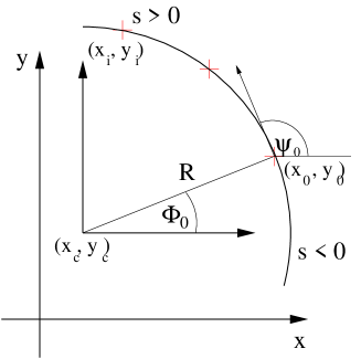
Figure A.1: Schematic view of the helix parameters. Projection of the helix in the $xy$-plane (left). Projection of the helix in the $sz$-plane (right).

Track fit parameters

The track fit in the transverse plane determines the center of curvature $(x_{c},y_{x})$ and the radius of curvature $R$, while the linear fit in $(s,z)$-plane returns the $z_{0}$ and $\tan\lambda$. In order to calculate the various track parameters, one need to determine the reference/starting point of the helix. This is typically chosen as a point closest to the innermost layer of the detector, i.e. relative to the innermost assigned space point of the track. If the innermost assigned space point on the track is ($x_{1},y_{1}$), the azimuthal angle can be defined as

$$\Phi_{0}=\tan^{-1}\frac{y_{1}-y_{c}}{x_{1}-x_{c}}.$$ (A.6)

The closest point $(x_{0},y_{0})$ on the trajectory and the azimuthal angle of the track direction at that point are then calculated according to

$$x_{0} = x_{c}+\frac{\cos\Phi_{0}}{\kappa}$$

$$y_{0} = y_{c}+\frac{\sin\Phi_{0}}{\kappa}$$

$$\psi_{0} = \Phi_{0}+h\frac{\pi}{2}$$ (A.7)

The remaining track parameters can be calculated as

$$p_{t} = \frac{KB}{\kappa}$$

$$p_{z} = p_{t}\tan\lambda$$

$$p = \sqrt{p_{t}^{2}+p_{z}^{2}}.$$ (A.8)

Helix going through origin

If the helix is going through the origin (0,0,0), the helix parameterization in equation A.5 is reduced to

$$x(s) = \frac{1}{\kappa}[\cos(\Phi_{0}+hs\kappa\cos\lambda)-\cos\Phi_{0}]$$

$$y(s) = \frac{1}{\kappa}[\sin(\Phi_{0}+hs\kappa\cos\lambda)-\sin\Phi_{0}]$$

$$z(s) = s\sin\lambda$$ (A.9)

Defining $t=s\kappa\cos\lambda$, and utilizing the relations

$$\cos(\Phi_{0}) = \cos(\psi_{0}-h\frac{\pi}{2})=h\sin\psi_{0}$$

$$\sin(\Phi_{0}) = \sin(\psi_{0}-h\frac{\pi}{2})=-h\cos\psi_{0}$$ (A.10)

gives

$$x(t) = \frac{1}{\kappa}[\sin(\psi_{0}+ht)-\sin\psi_{0}]$$

$$y(t) = \frac{1}{\kappa}[-\cos(\psi_{0}+ht)+\cos\psi_{0}]$$

$$z(t) = \gamma t$$ (A.11)

where

$$\gamma=\frac{\tan\lambda}{\kappa}$$ (A.12)

In this case the number of independent parameters describing the helix is reduced from five to 3, i.e. two parameters for the circular projection in the transverse plane ($\kappa$ and $\psi_{0}$), and one parameter for describing the longitudinal motion ($\gamma$).

Defining the track parameters at DCAO

The reference point of the track can be defined as the point of distance of closest approach to the coordinate system origin (DCAO), Figure A.2. This is useful if e.g. all tracks should be defined relative to the same point. In this case, the point $(x_{1},y_{1})$ in equation A.6 is (0,0) and $(x_{0},y_{0},z_{0})$ is the point at DCAO. The helix can now be defined by the parameter set,

$$(\kappa,r_{\mathrm{DCAO}},\phi_{\mathrm{DCAO}},z_{\mathrm{DCAO}},\lambda)$$

where $r_{\mathrm{DCAO}}$, $\phi_{\mathrm{DCAO}}$ and $z_{\mathrm{DCAO}}$ denotes the radius, azimuthal angle and z-coordinate at the point, respectively. In addition to these five parameters, two signs are needed to denote the sense of rotation, $h$, and the relative distance of the point with respect to the center of curvature (sign($R-\sqrt{x_{c}^{2}+y_{c}^{2}}$)). The five parameters thus completely define the helix, and the track parameters can be calculated as

$$x_{0} = |r_{\mathrm{DCAO}}|\cos\phi_{\mathrm{DCAO}}$$

$$y_{0} = |r_{\mathrm{DCAO}}|\sin\phi_{\mathrm{DCAO}}$$

$$\Phi_{0} = \left\{\begin{array}[]{ll}\phi_{\mathrm{DCAO}}&\mbox{if $R>\sqrt{x_{c}^{2}+y_{c}^{2}}$}\\ \phi_{\mathrm{DCAO}}+\frac{\pi}{2}&\mbox{if $R<\sqrt{x_{c}^{2}+y_{c}^{2}}$}\end{array}\right.$$ (A.15)

$$\psi_{0} = \Phi_{0}+h\frac{\pi}{2}$$

$$x_{c} = x_{0}-\frac{1}{\kappa}\cos\Phi_{0}$$

$$y_{c} = y_{0}-\frac{1}{\kappa}\sin\Phi_{0}$$ (A.16)

Figure A.2: Defining the track parameters at the point of DCAO.

Appendix B Software and data formats

B.1 Analysis software structure

All the HLT analysis software has been written in C++. The various processing steps are implemented in individual modules, allowing various processing topologies to be implemented. The data structures used internally in the framework are simple C-structures which has been adapted to the format which is likely to be used in the readout chain. In order to be compatible with the modular communication framework to be used in the HLT system (page 3.3), the data payloads between the processing modules are communicated by data references to the actual data in memory. This means that each module takes a data pointer as input, and reads the input data from corresponding location in memory. Similarly, the output data is written back to memory and the corresponding data pointer is communicated to the next module in the processing chain. This concept is illustrated in Figure B.1.

Figure B.1: Schematic overview of the data payload communication in the HLT reconstruction chain. In the online mode the communication is handled by the Publisher/Subscriber framework (left), while in offline mode the memory handling is handled transparently by a dedicated memory handler class (right).

When running the chain on a parallel prototype system (online mode), the inter-process communication is completely handled within the Publisher/Subscriber framework [56]. This framework is responsible for connecting all the various modules in the chain together, and the data payloads are handled transparent of the underlying network interface. For code development and tracking performance evaluation purposes/debugging etc, i.e. when running the chain in offline mode, the memory handling is done by a dedicated memory handler class. In this case, the output data is written to binary files for subsequent evaluation. In this way there is no difference between the two running modes as far as the processing modules are concerned. This makes it possible to use the same analysis code both for prototype testing of the HLT system and offline evaluation within the AliROOT framework.

Interface to AliROOT

The interface between the HLT and AliROOT framework is provided via special functions incorporated into a derived class of the HLT memory handling class. This functionality enables reading of the AliROOT data containers and transforming the data into the format used within the HLT framework, Figure B.2.

Figure B.2: Schematic overview of the interface between HLT analysis code and AliROOT.

This furthermore enables storing and sending the Monte Carlo information from the simulation through the HLT reconstruction chain in order to evaluate the tracking performance.

The HLT code can be compiled into shared libraries which can be loaded into an AliROOT interactive session where it can run and evaluated using standard ROOT-macros. The AliROOT support is controlled via preprocessor options during compiling.

B.2 Compressed data formats

8-bit RLE ADC-data format

In order to enable a simple approach to estimate the raw-data event sizes, a RLE ADC-data formatting scheme has been implemented. The format basically consists of replacing the zero-intervals between the sequences by a tag and the length of the intervals, and will therefore be comparable in size with the ALTRO-format.

Initially the 10 bit ADC-data from the simulation is converted to 8 bit using a 10-to-8 bit conversion table, Figure 5.1. The data is then compressed by the RLE scheme and written to binary files. The data is organized by its inherit granularity from the detector readout scheme, i.e. 1 file per (sub-)sector. Each file thus contains a certain number of pad-rows which is written in the beginning of the file. The remaining data stream consists of the data on the successive pad-rows,

NROWS PADROW_0 PADROW_1 ...

For every pad-row, PADROW_#, the corresponding row number is written together with the number of pads containing data on that row. (pads which has at least 1 sequence of time-bins above threshold) Both number are written using a 8 bit word, as the number of rows and pads on a given pad-row is 159 and 140, respectively. For every pad containing data the pad number is written, and then the ADC-values on that pad. When a series of zeros occur, a zero is written followed by the number of zeros. Example:

PAD 0 NZEROS ADC ADC ADC ADC 0 NZEROS ADC ADC ADC 0 0

This pad with number PAD contains two sequences with 4 and 3 consecutive time-bins respectively. The two zeros at the end is used to mark the end of the data stream on that pad. Each entry consists of a 8 bit word. If the number of zeros in a sequence is more than 255, an additional 8 bit word is written.

Bitwise I/O handling

For the implemented data compression schemes, bitwise handling of the data is necessary. The standard C I/O libraries only accommodates I/O on even byte boundaries, and all bitwise I/O has to be done using bitwise operators on integer values. In order to enable a more conventional way of handling bitwise I/O to files, special routines has been adapted from [82]. All bitwise I/O operations to file is done via the structure:

#include <stdio.h>
typedef struct bit_file {
    FILE *file;
    unsigned char mask;
    int rack;
} BIT_FILE;

All data is read/written to file via a pointer to the normal FILE structure. The bitwise handling of the data is done with the additional mask and rack elements. The rack contains the current byte of data either read in from the file or waiting to be written out to the file. mask contains a single bit mask used either to set or clear the current output bit or to mask in the current input bit. The mask element is initialized to 0x80, and during the output the first write to the BIT_FILE will set or clear that bit and the mask element shifts to the next. Once the mask has shifted to the point at which all the bits in the output rack have been set or cleared, the rack is written out to the file, and a new rack byte is started. Performing input from a BIT_FILE is done in a similar fashion.

Four types of I/O routines are defined, which read or write a single bit or multiple bits at a time:

void          OutputBit( BIT_FILE *bit_file, int bit );
void          OutputBits( BIT_FILE *bit_file,
                          unsigned long code, int bit_count );
int           InputBit( BIT_FILE *bit_file );
unsigned long InputBits( BIT_FILE *bit_file, int bit_count );

code denotes the value which is read/written using bit_count number of bits.

Compressed cluster data format

The compressed cluster data format has been used for the estimation of the data size needed to store the clusters as raw-data-arrays, Section 5.5.1. For every pad-row the corresponding row-number is written with a 8 bit word. Next the number of clusters present on the row is encoded with 10 bits. The data stream for a single pad-row then becomes:

PADROW NCLUSTERS CLUSTER CLUSTER CLUSTER ...

E.g. for a given pad-row the two first is written to the output file by:

OutputBits(bitfile,padrow,8);        //Padrow number
OutputBits(bitfile,n_clusters,10);   //Number of clusters on padrow

where

BIT_FILE *bitfile;     //Pointer set to the to the output file.

A cluster on the current pad-row is now written as

OutputBits(bitfile,pad_centroid,n_pad_bits);    //Pad centroid
OutputBits(bitfile,time_centroid,n_time_bits);  //Time centroid
OutputBits(bitfile,pad_width,n_padwidth_bits);  //Pad width
OutputBits(bitfile,time_width,n_timewidth_bits);//Time width
OutputBits(bitfile,tot_charge,n_charge_bits);   //Cluster charge

Compressed cluster–track data format

This format refers to the format used for the compressed track and cluster information, Section 5.5.2. It basically consists of the track parameters and the clusters assigned to the given track. The overall data stream has the following format

TRACK CLUSTER CLUSTER CLUSTER ... CLUSTER _CLEAR_

where TRACK and CLUSTER denotes the track and relative cluster parameters respectively. _CLEAR_ marks that the current bit-racks in BIT_FILE is written to file and the mask element is cleared.

The track parameters are defined within a standard C-structure as:

struct AliL3TrackModel {
  Float_t fKappa; //curvature
  Float_t fPhi;   //azimuthal angle of DCAO
  Float_t fD;     //radius of DCA0
  Float_t fZ0;    //z-coordinate of DCA0
  Float_t fTgl;   //tan of dipangle
};
typedef struct AliL3TrackModel AliL3TrackModel;

For a given track the parameters are written to the output file:

fwrite(&track,sizeof(AliL3TrackModel),1,bitfile->file);

where

BIT_FILE *bitfile;     //Pointer set to the to the output file.
AliL3TrackModel track; //Structure filled with the track parameters

The first cluster in the stream is encoded as:

OutputBit(bitfile,1);        //A single bit to flag cluster presence
OutputBits(bitfile,sector,6); //TPC sector number of the first cluster
OutputBit(output,0);                              //Sign of time residual
OutputBits(output,abs(delta_time_q),n_time_bits); //Absolute timeresidual value
OutputBit(output,0);                              //Sign of pad residual
OutputBits(output,abs(delta_pad_q),n_pad_bits);   //Absolute padresidual value
OutputBits(output,tot_charge,n_charge_bits);      //Cluster charge

The following clusters in the track list are encoded in the same fashion, with the only difference that instead of writing the TPC sector number for every cluster, a single bit is used to denote a possible change of sector. E.g. if there is no change:

OutputBit(bitfile,1); //Cluster present
OutputBit(bitfile,0); //No change of sector
OutputBit(output,0);                              //Sign of time residual
...

and if there was a change of sector

OutputBit(bitfile,1); //Cluster present
OutputBit(bitfile,1); //Change of sector
OutputBits(bitfile,sector,6); //New TPC sector number
OutputBit(output,0);                              //Sign of time residual
...

Reading/uncompressing the data is done similarly, using the corresponding input routines.

Bibliography

- [1] M. Gell-Mann, Phys. Rev. Lett. 8 (1964) 214.
- [2] G. Zweig, CERN Report 8419/TH (1964) 412.
- [3] T. Nakano et. al., Phys. Rev. Lett. 91 (2003) 012002.
- [4] V. V. Barmin et. al., Phys. Atom. Nucl. 66 (2003) 1715-1718.
- [5] S. Stepanyan et. al., Phys. Rev. Lett. 91 (2003) 252001.
- [6] J. Barth et. al., Evidence for the positive-strangeness pentaquark in photoproduction with the SAPHIR detector at ELSA, Preprint: arXiv:hep-ex/0307083.
- [7] C. Alt et. al., Phys. Rev. Lett. 92 (2004) 042003.
- [8] N. Cabbibo, G. Parisi, Phys. Lett. 59B (1975) 67.
- [9] K. G. Wilson, Phys. Rev. D10 (1974) 2445.
- [10] F. Karsch et. al., Phys. Lett. B478 (2000) 447.
- [11] R. D. Pisarki, F. Wilczek, Phys. Rev. D29 (1984) 338.
- [12] F. Karsch, Nucl. Phys. A698 (2002) 199.
- [13] Z. Fodor et. al. Phys. Lett. B568 (2003) 73.
- [14] J. D. Bjorken, Phys. Rev. D27 (1983) 140-151.
- [15] K. J. Eskola et. al., Nucl. Phys. A696 (2001) 715-728.
- [16] N. S. Amelin et. al., Eur. Phys. Jour. C22 (2001) 149-163.
- [17] U. Heinz, Nucl. Phys. A638 (1998) 357c.
- [18] R. Stock, Nucl. Phys. Lett. 456 (1999) 277.
- [19] J. Stachel, Nucl. Phys. A654 (1999) 119c.
- [20] U. Heinz, Nucl. Phys. A685 (2001) 414c.
- [21] R. Snellings et. al., Elliptic flow measurements from STAR, Preprint: arXiv:nucl-ex/0305001.
- [22] M. Becattini et. al., Eur. Phys. Jour. C5 (1998) 143.
- [23] S. Jeon, V. Koch, Phys. Rev. Lett. 85 (2000) 2076.
- [24] M. M. Aggarwal et. al., Phys. Rev. Lett. (1999) 83.
- [25] Justin Frantz et. al., Direct Photons in 200 GeV p+p and Au+Au Collisions, Presented at Quark Matter 2004, Oakland.
- [26] I. Arsene et. al., Phys. Rev. Lett. 91 (2003) 072305.
- [27] X. -N. Wang, M. Gyulassy, Phys. Rev. D44 (1991) 3501-3516.
- [28] X. N. Wang, Phys. Rev. C63 (2001) 054902.
- [29] Y. L. Dokshitzer, D. E. Kharzeev, Phys. Lett. B519 (2001) 199-206.
- [30] J. Adams et. al., Phys. Rev. Lett. 91 (2003) 072304.
- [31] The ALICE Collaboration, ALICE Physics Performance Report, Vol. I, CERN–LHCC–2003–049.
- [32] The ALICE Collaboration, Technical Proposal CERN–LHCC–1995–71.
- [33] The ALICE Collaboration, Technical Proposal, Addendum 1, CERN–LHCC–1996–32.
- [34] The ALICE Collaboration, Technical Proposal, Addendum 2, CERN–LHCC–1999–13.
- [35] The ALICE Collaboration, ALICE Technical Design Report for the Time Projection Chamber, CERN–LHCC–2000–001.
- [36] The ALICE Collaboration, ALICE Technical Design Report of the Transition Radiation Detector, CERN–LHCC–2001–021.
- [37] The ALICE Collatoration, ALICE Technical Design Report of the Time Of Flight System, CERN–LHCC–2000–12.
- [38] The ALICE Collaboration, Addendum to the ALICE Technical Report of the Time of Flight System, CERN–LHCC–2002–016.
- [39] The ALICE Collaboration, ALICE Technical Design Report of the Photon Multiplicity Detector, CERN–LHCC–1999–32.
- [40] The ALICE Collaboration, ALICE Technical Design Report of the Dimuon Forward Spectrometer, CERN–LHCC–1999–22.
- [41] The ALICE Collaboration, Addendum to the ALICE Technical Report for the Dimuon Forward Spectrometer, CERN–LHCC–2000–046.
- [42] The ALICE Collaboration, ALICE Technical Design Report of the Inner Tracking System, CERN–LHCC–1999–12.
- [43] The ALICE Collaboration, ALICE Technical Design Report of the Zero Degree Calorimeter, CERN–LHCC–1999–5.
- [44] The ALICE Collaboration, ALICE Technical Design Report of the Photon Spectrometer, CERN–LHCC–1999–4.
- [45] The ALICE Collaboration, ALICE Technical Design Report of the Detector for High Momentum PID, CERN–LHCC–1998–19.
- [46] G. Rai et. al., IEEE Trans. Nucl. Sci. NS-37 (1990) 56.
- [47] S. Afanasiev et. al., Nucl. Instrum. Meth. A430 (1999) 21.
- [48] M. Anderson et. al., Nucl. Instrum. Meth. A499 (2003) 659-678.
- [49] T. Lohse, W. Witzeling, The Time Projection Chamber, ALEPH–1991–156.
- [50] L. Musa, Nucl. Phys. A715 (2003) 843c-848c.
- [51] The ALICE Collaboration, Technical Design Report: Trigger, Data Acquisition, High-Level Trigger, Control System, CERN–LHCC–2003–062.
- [52] G. Paic et. al., Physics Requirement for the ALICE DAQ system, ALICE–INT–2000–30.
- [53] A. Dainese, Charm production and in-medium QCD energy loss in nucleus-nucleus collisions with ALICE. A performance study., Preprint: arXiv:nucl-ex/0311004.
- [54] F. Manso, A first algorithm for a dimuon High Level Trigger, ALICE–INT–2002–04.
- [55] J. Berger et. al., Nucl. Instr. Meth. A489 (2002) 406.
- [56] T. M. Steinbeck, A Modular Fault-Tolerant Data Transport Framework, Ph.D. thesis, Kirchhoff Institute of Physics, Ruprecht-Karls-University, Heidelberg, 2004.
- [57] M. Ohlsson et. al., Comp. Phys. Commun. 71 (1992) 77.
- [58] M. Gyulassy, M. Harlander, Comp. Phys. Commun. 66 (1991) 31-46.
- [59] B. Lasiuk et. al., Development of an Elastic Tracking Package, Proc. International Conference on Computing in High Energy Physics, Chicago, USA (1998).
- [60] P. V. C. Hough, Machine Analysis of Bubble Chamber Pictures, Proc. International Conference on High Energy Accelerators and Instrumentation, CERN (1959).
- [61] P. Billior, Nucl. Instrum. Meth. 225 (1984) 602.
- [62] R. Frühwirth, Application of Filter Methods to the Reconstruction of Tracks and Vertices in Events of Experimental High Energy Physics, HEPHY–PUB–516–88, Vienna (1988).
- [63] B. Batyunya et. al., Kalman Filtering Application for Track Recognition and Reconstruction in ALICE Tracking System, ALICE–INT–1997–24.
- [64] J. J. Hopfield, Proc. Nat. Acad. Sci. USA 79 (1982) 2554-2558.
- [65] G. Stimpfl-Abele, L. Garrido, Comp. Phys. Commun. 64 (1991) 46-56.
- [66] R. L. Gluckstern, Nucl. Instrum. Meth. 24 (1963) 381.
- [67] http://AliSoft.cern.ch/offline
- [68] http://root.cern.ch
- [69] F. Abe et. al., Phys. Rev. Lett. 61 (1988) 1819.
- [70] M. Kowalski, ALICE TPC Slow Simulator, ALICE–INT–1996–36.
- [71] Y. Belikov et. al., TPC tracking and particle identification in high-density environment, Preprint: arXiv:physics/0306108.
- [72] C. Adler et. al., Nucl. Instrum. Meth. A499 (2003) 778.
- [73] G. Grastveit et. al., FPGA Co-processor for the ALICE High Level Trigger, Preprint: arXiv:physics/0307017.
- [74] P. Yepes, Nucl. Instrum. Meth. A380 (1996) 582.
- [75] N. I. Chernov, G. A. Oskov, Comp. Phys. Commun. 33 (1984) 329-333.
- [76] D. W. Marquardt, Journal of the Society for Industrial and Applied Mathemathics 11 (1963) 431-441.
- [77] J. Illingworth, J. Kittler, Computer Vision Graphics Image Process. 44 (1988) 87-116.
- [78] V. F. Leavers, Computer Vision Graphics Image Process. 58 (1993) 250-264.
- [79] W. C. Y. Lam et. al., Patt. Recog. Lett. 15 (1994) 1127-1135.
- [80] Marian Ivanov, CERN, Private communication.
- [81] D. A. Huffman, Proc. IRE 40 (9) (1952) 1098.
- [82] M. Nelson, J. L. Gailly, The Data Compression Book, M T Books, New York, 1996.
- [83] R. M. Gray, IEEE ASSP Magazine (1984) 4ff.
- [84] Y. Belikov, CERN, Private communication.
- [85] R. K. Bock et. al., Data Analysis Techniques for High Energy Physics Experiments, Cambrigde University Press, 1990.