Statistical characterization of the interchange-instability spectrum of a separable ideal-magnetohydrodynamic model system

Abstract

A Suydam-unstable circular cylinder of plasma with periodic boundary conditions in the axial direction is studied within the approximation of linearized ideal magnetohydrodynamics (MHD). The normal mode equations are completely separable, so both the toroidal Fourier harmonic index $n$ and the poloidal index $m$ are good quantum numbers. The full spectrum of eigenvalues in the range $1\leq m\leq m_{\mathrm{max}}$ is analyzed quantitatively, using asymptotics for large $m$, numerics for all $m$, and graphics for qualitative understanding. The density of eigenvalues scales like $m_{\mathrm{max}}^{2}$ as $m_{\mathrm{max}}\rightarrow\infty$. Because finite-$m$ corrections scale as $1/m_{\mathrm{max}}^{2}$, their inclusion is essential in order to obtain the correct statistics for the distribution of eigenvalues. Near the largest growth rate only a single radial eigenmode contributes to the spectrum, so the eigenvalues there depend only on $m$ and $n$ as in a two-dimensional system. However, unlike the generic separable two-dimensional system, the statistics of the ideal-MHD spectrum departs somewhat from the Poisson distribution, even for arbitrarily large $m_{\mathrm{max}}$. This departure from Poissonian statistics may be understood qualitatively from the nature of the distribution of rational numbers in the rotational transform profile.

I Introduction

The general aim of this paper is to compare and contrast the spectrum of eigenvalues in typical integrable wave systems (e.g. waves in a rectangular cavity Casati et al. (1985)) with the spectrum of instabilities in a cylindrical plasma within the ideal magnetohydrodynamics (MHD) approximation. This is a first step in understanding the spectral problem in the complex three-dimensional geometry of the class of magnetic confinement fusion experiments known as stellarators Wakatani (1998).

In ideal MHD the spectrum of the frequencies, $\omega$, of normal modes of displacements about a toroidal equilibrium is difficult to characterize mathematically because the linearized force operator is not compact Lifschitz (1989). In addition to a point (discrete) spectrum of unstable modes ($\omega^{2}<0$) there are the Alfvén and slow-magnetosonic continuous spectra on the stable side of the origin ($\omega^{2}>0$) and the possibility of dense sets of accumulation points on the unstable side. In mathematical spectral theory the stable continua and unstable accumulation “continua” Spies and Tataronis (2003) are characterized Hameiri (1985) as belonging to the essential spectrum. (For a self-adjoint operator $L$, the essential spectrum is the set of $\lambda$-values for which the range of $L-\lambda$ is not a closed set and/or the dimensionality of the null space of $L-\lambda$ is infinite.)

There is experimental evidence that ideal MHD is relevant in interpreting experimental results Troyon et al. (1984); Ferron et al. (2000), but perhaps the greatest virtue of ideal MHD in fusion plasma physics is its mathematical tractability as a first-cut model for assessing the stability of proposed fusion-relevant experiments with complicated geometries in the pre-design phase.

For this purpose a substantial investment in effort has been expended on developing numerical matrix eigenvalue programs, such as the three-dimensional TERPSICHORE Anderson et al. (1990) and CAS3D Schwab (1993) codes. These solve the MHD wave equations for perturbations about static equilibria, so that the eigenvalue $\omega^{2}$ is real due to the Hermiticity (self-adjointness Bernstein et al. (1958)) of the linearized force and kinetic energy operators. They use finite-element or finite-difference methods to convert the infinite-dimensional PDE eigenvalue problem to an approximating finite-dimensional matrix problem. An alternative approach is to use local analysis using the ballooning representation and to attempt semiclassical quantization to estimate the global spectrum Dewar and Glasser (1983); Cuthbert et al. (1998); Redi et al. (2002).

In order properly to verify the convergence of these codes in three-dimensional geometry it is essential to understand the nature of the spectrum—if it is quantum-chaotic then convergence of individual eigenvalues cannot be expected and a statistical description must be used Gutzwiller (1990); Mehta (1991); Stöckmann (1999); Haake (2001).

This is perhaps of most importance in understanding the spectrum in three-dimensional magnetic confinement geometries, in particular the various stellarator experiments currently running or under construction. These devices are called three-dimensional because they possess no continuous geometrical symmetries, and thus there is no separation of variables to reduce the dimensionality of the eigenvalue problem. It has been shown Dewar et al. (2001) that the semiclassical limit (a Hamiltonian ray tracing problem) for ballooning instabilities in such geometries may be strongly chaotic because there are no ignorable coordinates in the ray Hamiltonian.

However, the present paper discusses the opposite limit, a system with a sufficient number of symmetries to make the ray Hamiltonian integrable and the eigenvalue problem separable. The geometry is the circular cylinder, periodic in the $z$-direction to make it topologically toroidal—we shall refer to the $z$-direction as the toroidal direction and the azimuthal, $\theta$-direction as the poloidal direction. The study of this separable system will provide a baseline for comparison with the three-dimensional toroidal case in future work. The overall goal of the paper is to determine if the ideal-MHD spectrum falls within the same universality class as that of typical waves in separable geometries or, if not, what might cause it to differ.

Berry and Tabor Berry and Tabor (1977) show that the distribution function $P(s)$ for the spacing of adjacent energy levels (suitably scaled) in a generic separable quantum system with more than one degree of freedom is $\exp(-s)$, as for a Poisson process with levels distributed at random. They also show that the spectrum of uncoupled quantum oscillators is nongeneric even when the frequency ratios are not commensurate, in which case $P(s)$ peaks about a nonzero value of $s$ (as also occurs in nonintegrable, chaotic systems—the “level repulsion” effect). A more surprising departure from the Poisson distribution was found by Casati et al. Casati et al. (1985) for waves in a rectangular box with irrational aspect ratio, but the departure was very small. Level spacing statistics are discussed also in the standard monographs on quantum chaos Gutzwiller (1990); Mehta (1991); Stöckmann (1999); Haake (2001).

In contrast with quantum mechanics, where the continuous spectrum arises from the unboundedness of configuration space, the ideal-MHD essential spectrum arises from the unboundedness of Fourier space—there is no minimum wavelength. This is an unphysical artifact of the ideal MHD model because, in reality, low-frequency instabilities with $|{\mathbf{k}}_{\perp}|$ much greater than the ion Larmor radius, $a_{\mathrm{i}}$, cannot exist (where ${\mathbf{k}}_{\perp}$ is the projection of the local wavevector into the plane perpendicular to the magnetic field ${\mathbf{B}}$). Indeed, ideal MHD breaks down in various ways at large $|{\mathbf{k}}_{\perp}|$, with dissipative and drift effects coming into play.

In this paper we do not attempt to model finite-Larmor-radius stabilization, but instead simply restrict the poloidal mode spectrum to $m\leq m_{\mathrm{max}}$ and study the scaling of the spectrum at large $m_{\mathrm{max}}$. The nature of the dispersion relation is such that the toroidal mode numbers $n$ relevant to the spectrum are also restricted. In a matrix eigenvalue code such as CAS3D or TERPSICHORE our procedure corresponds to using an arbitrarily fine radial mesh but truncating the toroidal and poloidal basis set.

The eigenvalue equation for a reduced MHD model of a stellarator is presented in Sec. II. We study a plasma in which the Suydam criterion Suydam (1958) for the stability of interchange modes is violated, so the number of unstable modes is infinite.

Section III is devoted to developing an understanding of the dependence (the dispersion relation) of the eigenvalues on the radial, poloidal and toroidal mode numbers, $l$, $m$, and $n$, respectively. As $m$ and $n$ approach infinity, keeping $\mu\equiv n/m$ fixed, the growth-rate eigenvalues asymptote to a constant, the Suydam growth rate, depending only on $\mu$ and the radial mode number $l$. We use a combination of perturbation expansion in $1/m$ and numerical solution of the eigenvalue equation using a new transformation to Schrödinger form that is applicable over the whole range of $m$, from $O(1)$ to $\infty$. This generalizes the approach of Cheremhykh and Revenchuk Cheremhykh and Revenchuk (1992), which was limited to the $m=\infty$ Suydam eigenvalue problem. We compare some of the asymptotic results in Cheremhykh and Revenchuk (1992) with our numerical solutions. Our perturbation expansion shows that the correction to the Suydam limit goes as $1/m^{2}$. Contrary to usual experience Sugama and Wakatani (1989), our numerical solutions show that the growth rates do not always approach the Suydam values from below as $m\rightarrow\infty$.

In Sec. IV we examine the part of the spectrum involving the most unstable modes, which is essentially two-dimensional because only the lowest-order radial mode, $l=0$, contributes. We relate the considerable amount of structure observed in the spectrum to the Farey sequences of rational values of the rotational transform (winding number) of the equilibrium magnetic field. Low-order rationals have associated eigenvalue sequences giving a regular distribution of eigenvalues locally more like the spectrum of a one-dimensional system than a two-dimensional one.

In Sec. V we derive the analog of the Weyl formula for the average density of states, including an asymptotic analysis of the large-$l$ limit. In Sec. VI we show level spacing distributions $P(s)$. Since we are interested in large $m$ we first try approximating the eigenvalues by their corresponding asymptotic Suydam limit. This gives a very singular distribution with a delta-function-like spike at the origin Dewar et al. (2004) due to the extremely degenerate nature of the spectrum in this approximation. By contrast the distribution for the exact spectrum has no spike at the origin, showing that the small $1/m^{2}$ corrections break the degeneracy sufficiently to completely change the statistics.

We examine the statistics for the $l=0$ and $l=1$ spectra, both individually and combined (in the low-growth-rate region where they overlap). We have examined sufficiently large data sets to show convincingly that the statistical distributions are not Poissonian, though that of the combined $l=0$ and $l=1$ spectrum is closest. We also split the $l=0$ spectrum into two halves to remove overlap of spectra arising from different parts of the plasma. These split spectra exhibit a much more dramatic departure from Poisson statistics, showing that the ideal-MHD interchange spectrum is indeed nongeneric in the sense of Berry and Tabor Berry and Tabor (1977).

II Choice of model eigenvalue equation

The grand context of this paper is the three-dimensional linearized ideal MHD problem—to solve, under appropriate boundary conditions, the equation of motion

$$\rho\partial_{t}^{2}{\bm{\xi}}={\mathbf{\mathsf{F}}}\cdot{\bm{\xi}}$$ (1)

for small displacements ${\bm{\xi}}({\mathbf{r}},t)$ of the MHD fluid about a static equilibrium state, where $\rho({\mathbf{r}})$ is the equilibrium mass density, ${\mathbf{r}}$ is position, $t$ is time, and ${\mathbf{\mathsf{F}}}$ is a Hermitian linearized force operator Bernstein et al. (1958) under the inner product $\int d^{3}x\,{\bm{\xi}}^{*}\mbox{\boldmath$\cdot$}{\mathbf{\mathsf{F}}}\mbox{\boldmath$\cdot$}{\bm{\xi}}$ and suitable boundary conditions. (Superscript * denotes complex conjugation—we can take ${\bm{\xi}}$ to be complex because all the coefficients in ${\mathbf{\mathsf{F}}}$ are real, so the real and imaginary parts of ${\bm{\xi}}$ obey the same equation.)

Most modern magnetic confinement fusion experiments, in particular tokamaks and stellarators, are toroidal. Though not guaranteed for arbitrary three-dimensional systems, the equilibrium magnetic field ${\mathbf{B}}({\mathbf{r}})$ is normally assumed to be integrable in the sense that all field lines lie on invariant tori (magnetic surfaces) nested about a single closed field line (the magnetic axis). Within each toroidal magnetic surface a natural angular coordinate system is set up, with the poloidal angle $\theta$ increasing by $2\pi$ for each circuit around the short way and the toroidal angle $\zeta$ increasing by $2\pi$ for each circuit the long way. Each surface is characterized by a magnetic winding number, the rotational transform $\iota\!\!$-, being the average poloidal rotation of a field line per toroidal circuit, $\langle d\theta/d\zeta\rangle$, over an infinite number of circuits. (In tokamak physics the inverse, $q\equiv 1/{\mbox{$\iota\!\!$-}}$, is normally used as the rotation number.)

In this paper we study an effectively circular-cylindrical MHD equilibrium, using cylindrical coordinates such that the magnetic axis coincides with the $z$-axis, made topologically toroidal by periodic boundary conditions. Thus $z$ and the toroidal angle $\zeta$ are related through $\zeta\equiv z/R_{0}$, where $R_{0}$ is the major radius of the toroidal plasma being modeled by this cylinder. The poloidal angle $\theta$ is the usual geometric cylindrical angle and the distance $r$ from the magnetic axis labels the magnetic surfaces (the equilibrium field being trivially integrable in this case). The plasma edge is at $r=a$.

In the cylinder there are two ignorable coordinates, $\theta$ and $\zeta$, so the components of ${\bm{\xi}}$ are completely factorizable into products of functions of the independent variables separately. In particular, we write the $r$-component as

$$r\xi_{r}=\exp(im\theta)\exp(-in\zeta)\varphi(r)\;,$$ (2)

where the periodic boundary conditions quantize $m$ and $n$ to integers and we choose to work with the stream function $\varphi(r)\equiv r\xi_{r}(r)$.

Since the primary motivation of this paper is stellarator physics, we use the reduced MHD ordering for large-aspect stellarators Strauss (1980); Wakatani (1998), averaging over helical ripple to reduce to an equivalent cylindrical problem Kulsrud (1963); Tatsuno et al. (1999). The universality class should be insensitive to the precise choice of model as long as it exhibits the behavior typical of MHD instabilities in a cylindrical plasma, specifically the existence of interchange instabilities and the occurrence of accumulation points at finite growth rates.

We nondimensionalize by measuring the radius $r$ in units of the minor radius of the plasma column, $a$, and the time $t$ in units of the poloidal Alfvén time $\tau_{\mathrm{A}}=R_{0}\sqrt{\mu_{0}\rho}/B_{0}$, where $B_{0}$ is the toroidal magnetic field and $\mu_{0}$ is the permeability of free space. Thus $\omega$ is in units of $\tau_{\rm A}^{-1}$. Defining $\lambda\equiv\omega^{2}$ we seek the spectrum of $\lambda$-values satisfying the scalar equation

$$L\varphi=\lambda M\varphi$$ (3)

under the boundary conditions $\varphi(0)=0$ at the magnetic axis and $\varphi(1)=0$, appropriate to a perfectly conducting wall at the plasma edge. The operators $L$ and $M$ given below are Hermitian under the inner product defined, for arbitrary functions $f$ and $g$ satisfying the boundary conditions, by

$$\langle f,g\rangle\equiv\int_{0}^{1}f^{*}(r)g(r)\;r\,dr\;.$$ (4)

The weight factor $r$ in the inner product is a Jacobian factor coming from $d^{3}x=rdrd\theta dz$.

The operator $L$ is given by

$$L \equiv -\frac{1}{r}\frac{d}{dr}(n-m{\mbox{$\iota\!\!$-}})^{2}r\frac{d}{dr}$$ (5)

$$\mbox{}+\frac{m^{2}}{r^{2}}\left[(n-m{\mbox{$\iota\!\!$-}})^{2}-D_{\mathrm{S}}+\frac{\ddot{{\mbox{$\iota\!\!$-}}}}{m}(n-m{\mbox{$\iota\!\!$-}})\right]\;,$$

where the Suydam stability parameter $D_{\mathrm{S}}$ is

$$D_{\mathrm{S}}\equiv-\frac{\beta_{0}}{2\epsilon^{2}}p^{\prime}(r)\Omega^{\prime}(r)\;,$$ (6)

with $\epsilon\equiv a/R_{0}\ll 1$ the inverse aspect ratio, $p(r)$ the plasma pressure normalized to unity at $r=0$, $\beta_{0}\equiv 2\mu_{0}p_{0}/B_{0}^{2}$ the ratio of plasma pressure to magnetic pressure at the magnetic axis, and $\Omega^{\prime}$ the average field line curvature. Here

$$\Omega\equiv\epsilon^{2}N\left(r^{2}{\mbox{$\iota\!\!$-}}+2\int r{\mbox{$\iota\!\!$-}}dr\right)$$ (7)

where the rotational transform is produced by helical current windings making $N\gg 1$ turns as $\zeta$ goes from $0$ to $2\pi$, $\Omega^{\prime}(r)$ giving the averaged field-line curvature. (Note that $\epsilon$ cancels out in $D_{\mathrm{S}}$.) We use the notation $\dot{f}\equiv rf^{\prime}(r)$ for an arbitrary function $f$, so $\dot{{\mbox{$\iota\!\!$-}}}\equiv rd{\mbox{$\iota\!\!$-}}/dr$ is a measure of the magnetic shear and $\ddot{{\mbox{$\iota\!\!$-}}}$ measures the variation of the shear with radius. The term $\Omega$ is a measure of the “magnetic hill” Wakatani (1998) that allows pressure energy to be released by interchanging field lines, thus driving the interchange instability.

The operator arising from the inertial term in Eq. (1),

$$M\equiv-\nabla_{\perp}^{2}=-\frac{1}{r}\frac{d}{dr}r\frac{d}{dr}+\frac{m^{2}}{r^{2}}\;,$$ (8)

is easily seen to be positive definite under the inner product Eq. (4).

We observe some differences between Eq. (3) and the standard quantum mechanical eigenvalue problem $H\psi=E\psi$. One is of course the physical interpretation of the eigenvalue—in quantum mechanics the eigenvalue $E\equiv\hbar\omega$ is linear in the frequency because the Schrödinger equation is first order in time, whereas our eigenvalue $\lambda$ is quadratic in the frequency because it derives from a classical equation of motion.

Another difference is that Eq. (3) is a generalized eigenvalue equation because $M$ is not the identity operator. This is one reason why it is necessary to treat the MHD spectrum explicitly rather than simply assume it is in the same universality class as standard quantum mechanical systems.

Just as in ordinary eigenvalue problems the eigenvalue spectrum for the generalized eigenvalue problem is real, and the eigenfunctions $\varphi_{i}$ have a generalized orthogonality property

$$\langle\varphi_{i},M\varphi_{j}\rangle=\delta_{i,j}\;,$$ (9)

where the normalization has been chosen to make the coefficient of the Kronecker $\delta$ unity. Here $i$ and $j$ denote members of the set $\{l,m,n\}$, where $l$ is the radial node number and the poloidal and toroidal mode numbers $m$ and $n$, respectively, are defined in Eq. (2). The negative part of the spectrum, $\lambda=-\gamma^{2}<0$, corresponds to instabilities growing exponentially with growth rate $\gamma$.

Equation (3) is very similar to the normal mode equation analyzed in the early work on the interchange growth rate in stellarators by Kulsrud Kulsrud (1963). However, unlike this and most other MHD studies we are concerned not with finding the highest growth rate, but in characterizing the complete set of unstable eigenvalues.

III Interchange spectrum

In this section we discuss the standard unregularized ideal MHD spectrum. It is well known that for $\lambda>0$ the spectrum consists of the Alfvén continuum (the slow-magnetosonic continuum being removed in reduced MHD McMillan et al. (2004)). On the unstable side of the spectrum, $\lambda<0$, it is also known that there is an infinity of eigenvalues provided the Suydam interchange instability criterion Suydam (1958)

$$G\equiv\frac{D_{\mathrm{S}}}{\dot{{\mbox{$\iota\!\!$-}}}^{2}}>\frac{1}{4}$$ (10)

is satisfied over some range of $r$ in the interval $(0,1)$, but the details of the spectrum do not appear to have been published before.

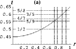
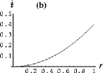
Figure 1: (a) The rotational transform ${\mbox{$\iota\!\!$-}}(r)\equiv 1/q(r)$ defined by Eq. (11) with ${\mbox{$\iota\!\!$-}}_{0}=0.45$, ${\mbox{$\iota\!\!$-}}_{2}=0.2$ (as for all subsequent plots); (b) the magnetic shear parameter $\dot{{\mbox{$\iota\!\!$-}}}\equiv r{\mbox{$\iota\!\!$-}}^{\prime}(r)$. In (a), all distinct rational magnetic surfaces ${\mbox{$\iota\!\!$-}}=\mu\equiv n/m$ are shown for $m$ up to 10.

III.1 Profiles

Interchange instabilities occur only for values of $m$ and $n$ such that $n-m{\mbox{$\iota\!\!$-}}$ vanishes (or at least can be made very small Tatsuno et al. (1999)) and therefore it is important to know something about the function ${\mbox{$\iota\!\!$-}}(r)$. The typical profile of ${\mbox{$\iota\!\!$-}}(r)$ in a stellarator is monotonically increasing in the interval $[0,a]$ and we shall assume this to be the case here (though it is not always true in modern stellarators). For the numerical work in this paper we use a parabolic profile

$${\mbox{$\iota\!\!$-}}={\mbox{$\iota\!\!$-}}_{0}+{\mbox{$\iota\!\!$-}}_{2}r^{2}$$ (11)

as illustrated in Fig. 1(a).

Given a rational fraction $\mu=n_{\mu}/m_{\mu}$ in the interval $[{\mbox{$\iota\!\!$-}}(0),{\mbox{$\iota\!\!$-}}(a)]$ (where $n_{\mu}$and $m_{\mu}$ are mutually prime) there is a unique radius $r_{\mu}$ such that ${\mbox{$\iota\!\!$-}}(r_{\mu})=\mu\;.$ Any pair of integers $(m,n)_{\mu,\nu}\equiv(\nu m_{\mu},\nu n_{\mu})$, $\nu=1,2,3,\ldots$ satisfies the resonance condition

$$n_{\mu,\nu}-m_{\mu,\nu}{\mbox{$\iota\!\!$-}}(r_{\mu})=0\;.$$ (12)

For example, the set of rationals with $1<m\leq 10$ in the interval of $\iota\!\!$- shown in Fig. 1(a) is $\{\mu\}=\{1/2,\;5/9,\;4/7,\;3/5,\;5/8\}$, as shown in the figure.

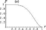
Figure 2: (a) The pressure profile $p(r)$, Eq. (13), used in this paper and (b) the Suydam criterion parameter $G(r)$, defined in Eq. (10) (solid line), and the instability threshold $1/4$ (dashed line), showing nearly all the plasma is interchange unstable.

To understand the global spectrum we also need to know something about the pressure profile. In this paper we use a broad pressure profile that is sufficiently flat near the magnetic axis that the Suydam instability parameter $G$ defined in Eq. (10) goes to zero at the magnetic axis, and for which $p^{\prime}$ vanishes at the plasma edge

$$p(r)=1-6\,r^{5}+5\,r^{6}\;.$$ (13)

This profile is shown in Fig. 2(a) and the resulting $G$-profile in Fig. 2(b).

III.2 High $m$ and $n$

In this subsection we choose a particular rational surface $r_{\mu}$ and restrict attention to pairs $(m,n)$ from the set $\{(m,n)_{\mu,\nu}|\nu=1,2,3,\ldots\}$ satisfying the condition Eq. (12).

Defining a scaled radial variable $x\equiv m(r-r_{\mu})/r_{\mu}$, we expand all quantities in inverse powers of $m$,

$$L \equiv \frac{m^{2}}{r_{\mu}^{2}}(L^{(0)}+m^{-1}L^{(1)}+m^{-2}L^{(2)}+\ldots)\;,$$

$$M \equiv \frac{m^{2}}{r_{\mu}^{2}}(M^{(0)}+m^{-1}M^{(1)}+m^{-2}M^{(2)}+\ldots)$$ (14)

Also, $\lambda=\lambda^{(0)}+m^{-1}\lambda^{(1)}+m^{-2}\lambda^{(2)}$, and similarly for $\varphi$. The detailed expressions are given in Appendix A .

We then solve Eq. (3) by equating the LHS to zero order by order. At $O(m^{0})$, as found by Kulsrud Kulsrud (1963), we have the generalized eigenvalue equation

$$\mathcal{L}^{(0)}\varphi^{(0)}=0\;,$$ (15)

where

$$\mathcal{L}^{(0)} \equiv L^{(0)}-\lambda^{(0)}M^{(0)}$$ (16)

$$= -\frac{d}{dx}(\dot{{\mbox{$\iota\!\!$-}}}^{2}x^{2}-\lambda^{(0)})\frac{d}{dx}+\dot{{\mbox{$\iota\!\!$-}}}^{2}x^{2}-\lambda^{(0)}-D_{\mathrm{S}}$$

with $\dot{{\mbox{$\iota\!\!$-}}}$ and $D_{\mathrm{S}}$ evaluated at $r_{\mu}$. For $\lambda^{(0)}<0$, Eq. (15) can be solved to give a square-integrable eigenfunction under the boundary conditions $\varphi^{(0)}\rightarrow 0$ as $r\rightarrow\pm\infty$ when $\lambda^{(0)}$ is one of the eigenvalues $\lambda_{\mu,l}$, $l=0,1,2,\ldots$, denoting the number of radial nodes of the eigenfunction $\varphi^{(0)}=\varphi_{\mu,l}$. Note that $\lambda_{\mu,l}$ depends only on $\mu=n/m$ and is otherwise independent of the magnitude of $m$ and $n$. We assume that the $\varphi_{\mu,l}(r)$, when combined with the continuum generalized eigenfunctions for $\lambda^{(0)}>0$, form a complete set.

III.2.1 Suydam approximation

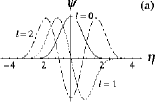
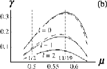
Figure 3: (a) $m=\infty$ eigenfunctions for the $l=0$ (solid line), $l=1$ (short dashes) and $l=2$ (short and long dashes) modes at $\mu=1/2$, arbitrary normalization. (b) Growth rates $\gamma$ vs. resonant ${\mbox{$\iota\!\!$-}}\equiv\mu$. Dashed lines show approximations Eq. (21) (for $l=0$) and Eq. (20) (for $l=1$ and $2$).

The leading term in the expansion of the eigenvalue in $1/m$ gives the growth rate in the limit $m\rightarrow\infty$, known as the Suydam approximation. Restricting attention to unstable modes, so that $\gamma\equiv(-\lambda)^{1/2}$ is real, we transform Eq. (15) to the Schrödinger form Cheremhykh and Revenchuk (1992)

$$\frac{d^{2}\psi}{d\eta^{2}}+Q(\eta)\psi=0\;,$$ (17)

where

$$Q=Q_{0}(\eta|\gamma,\mu)\equiv G-{\textstyle{\mathrm{\frac{1}{4}}}}-{\textstyle{\mathrm{\frac{1}{4}}}}\operatorname{sech}^{2}\,\eta-\Gamma^{2}\cosh^{2}\eta\;,$$ (18)

with $G\equiv G(r_{\mu})$ defined as in Eq. (10), $\Gamma\equiv\gamma/\dot{{\mbox{$\iota\!\!$-}}}(r_{\mu})$, $\eta$ defined through $x\equiv\gamma\sinh\eta/\dot{{\mbox{$\iota\!\!$-}}}(r_{\mu})$, and $\psi\equiv(\cosh\eta)^{1/2}\varphi(x)$. [In Ref. Cheremhykh and Revenchuk, 1992 Eq. (18) is derived from the Fourier transform of Eq. (15), but we can also use the real-space version as the equation shares with the quantum oscillator the remarkable property of having the same general form in both Fourier space and real space.]

Cheremhykh and Revenchuk Cheremhykh and Revenchuk (1992) (CR) have made an extensive study of the eigenvalues of Eq. (17) using the semiclassical quantization condition

$$\oint Q_{0}(\eta)^{1/2}\,d\eta=(2l+1)\pi\;.$$ (19)

which follows from the WKB ansatz $\psi=A(\eta)\exp\pm i\int Q_{0}^{1/2}\,d\eta$. CR derive several approximations, useful in appropriate limits, improving on the earlier result of Kulsrud Kulsrud (1963). In this paper we use two of their results to compare with numerical solutions of Eq. (17). The first is Eq. (4.5) of Cheremhykh and Revenchuk (1992)

$$\Gamma\approx\frac{4\sigma}{e}\exp\left[-\frac{(l+{\textstyle{\mathrm{\frac{1}{2}}}})\pi}{2\sigma}-\frac{1}{4\sigma^{2}}\right]\;,$$ (20)

which [combining the criteria given in CR’s Eqs. (4.4) and (4.12)] is applicable when $\sigma\equiv(G-1/4)^{1/2}\gg 1/2$. The second CR result we use is their Eq. (4.7)

$$\Gamma^{2}\approx\frac{G-(2l+1)G^{1/2}}{1+(4G)^{-1}}\;,$$ (21)

applicable when $G\gtrsim\Gamma^{2}\gg 1$.

As is seen from Fig. 3, Eq. (21) gives a remarkably good approximation to the growth rate of the most unstable radial eigenmode, $l=0$, and Eq. (20) gives a good approximation for the higher-$l$ modes (the semiclassical quantization being strictly justifiable only for large $l$). The growth-rate maxima for each $l$ occur close to the maximum of $G$ (and hence $\Gamma)$, but not exactly owing to the $\dot{{\mbox{$\iota\!\!$-}}}$ factor in the definition $\Gamma\equiv\gamma/\dot{{\mbox{$\iota\!\!$-}}}(r_{\mu})$.

From Eq. (21) we see that, provided the Suydam criterion $G>1/4$ is satisfied, there is an infinity of growth rate eigenvalues accumulating exponentially toward the origin from above (so the $\lambda$-values accumulate from below) in the limit $l\rightarrow\infty$.

Perhaps less widely appreciated (because $m$ and $n$ are normally taken to be fixed) is the fact that there is also a point of accumulation of the eigenvalues of Eq. (3) at each $\lambda_{\mu,l}$ as $m_{\mathrm{max}}\rightarrow\infty$ with $l$ fixed. To break the degeneracy of $\lambda^{(0)}$ we must proceed further with the expansion in $1/m$.

III.2.2 $1/m^{2}$ corrections

Proceeding with the expansion Eq. (14), the calculation goes through much as in standard time-independent quantum perturbation theory (Landau and Lifshitz, 1991, e.g.).

The lowest order eigenvalues and eigenfunctions are, as found in Sec. III.2, $\lambda^{(0)}=\lambda_{\mu,l}$ and $\varphi^{(0)}=\varphi_{\mu,l}(x)$, respectively. The $O(1/m)$ correction, $\lambda^{(1)}$, vanishes identically from parity considerations—$\varphi_{\mu,l}(x)$ is either an even or odd function so its contribution to the matrix elements of $L^{(1)}$ and $M^{(1)}$ between $\varphi^{(0)}$ and $\varphi^{(0)}$ is even. On the other hand, $L^{(1)}$ and $M^{(1)}$ are odd, so $\lambda^{(1)}\equiv 0$. (This contrasts with the finite-aspect-ratio toroidal case where toroidal coupling of Fourier harmonics of different $m$ to form ballooning modes leads to a nonvanishing $1/n$ correction Connor et al. (1979); Dewar et al. (1979).)

The first nonvanishing correction term is thus

$$\lambda^{(2)} = \langle\mu,l|\mathcal{L}^{(2)}|\mu,l\rangle$$ (22)

$$\mbox{}-\sum_{l^{\prime}\neq l}\frac{\langle\mu,l|\mathcal{L}^{(1)}|\mu,l^{\prime}\rangle\langle\mu,l^{\prime}|\mathcal{L}^{(1)}|\mu,l\rangle}{\lambda_{\mu,l^{\prime}}-\lambda_{\mu,l}}\;,$$

where the sum over $l^{\prime}$ is taken to include an integration over the continuum. The operators $\mathcal{L}^{(i)}\equiv L^{(i)}-\lambda_{\mu,l}M^{(i)}$ are the higher-order generalizations of $\mathcal{L}^{(0)}$, defined by Eq. (16). The $m=\infty$ matrix elements of any operator $\mathcal{F}$ are defined by

$$\langle\mu,l^{\prime}|\mathcal{F}|\mu,l^{\prime\prime}\rangle\equiv\int_{-\infty}^{\infty}\varphi_{\mu,l^{\prime}}^{*}(x)\mathcal{F}\varphi_{\mu,l^{\prime\prime}}(x)\;dx\;,$$ (23)

with the eigenfunctions $\varphi_{\mu,l}(x)$ being normalized so that $\langle\mu,l|M^{(0)}|\mu,l\rangle=1$. Note that, with the operators $L$ and $M$ defined as in Eqs. (5) and (8) , $\mathcal{L}^{(i)}$ is Hermitian under the inner product used in Eq. (23) only for $i=0$. However, it can be made Hermitian at arbitrary order by the redefinitions $L\mapsto rL$ and $M\mapsto rM$, which puts the eigenvalue equation into Sturm–Liouville form.

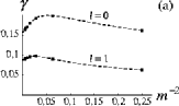
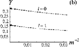
Figure 4: Growth rates $\gamma_{l,m,n}\equiv(-\lambda_{l,m,n})^{1/2}$ vs. $m^{-2}$ for $l=0$ and $1$, found by numerical solution of Eq. (3) (Sec. III.3): (a) $n/m=1/2$ ($m=2,4,6,\ldots$), and (b) $n/m=11/19$ ($m=19,38,57,\ldots$). At high $m$ the dependence becomes linear, in qualitative agreement with Sec. III.2.2.

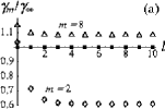
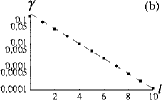
Figure 5: Growth rates vs. radial node number $l$: (a) found by numerical solution of Eq. (3) (Sec. III.3) for $(m,n)=(2,1)$ (diamonds) and $(8,4)$ (triangles), normalized to the $\mu=1/2$, infinite-$m$ results (filled boxes); (b) $\mu=1/2$, infinite-$m$ results (points) and asymptotic result Eq. (20) (dashed line).

As in quantum mechanics (Landau and Lifshitz, 1991, e.g.), if $\mathcal{L}^{(1)}$ is Hermitian the contribution of the second term on the right hand side of Eq. (22) is always negative for the lowest eigenvalue, $\lambda^{(0)}_{0}$, because $\lambda_{l^{\prime}}^{(0)}-\lambda_{l}^{(0)}>0$. However, in ideal MHD a positive contribution from the first term usually dominates and the infinite-$m$ mode is most unstable Sugama and Wakatani (1989). As seen in Fig. 4, this is not always the case: $\lambda^{(2)}_{l=0}$ is negative for $\mu=1/2$, but positive for $\mu=11/19=0.578947\ldots$.

The latter value of $\mu$ is very close to the value giving the global maximum Suydam growth rate (see Fig. 3). Thus, in the special case studied here and in accordance with conventional wisdom, the global maximum interchange growth rate occurs at $m=\infty$. Both these results are intuitively reasonable—the eigenfunctions become increasingly localized as $m\rightarrow\infty$, so the highest growth rate is obtained by localizing in the “most unstable” region of the plasma, where ${\mbox{$\iota\!\!$-}}\approx 11/19$. On the other hand, modes which localize in “less unstable” regions as $m\rightarrow\infty$ can achieve a higher growth rate at finite values of $m$ because their more extended finite-$m$ eigenfunctions overlap the more unstable region and tap into the free energy from the pressure gradient in this region.

Since the eigenvalues approach $\lambda_{\mu,l}$ as $1/m^{2}$, there is an infinity of modes in the neighborhood of each $\lambda_{\mu,l}$ in the limit $m_{\mathrm{max}}\rightarrow\infty$. That is, they are finite-growth-rate accumulation points of the complete spectrum. Because the rationals $\mu$ are dense on the interval $({\mbox{$\iota\!\!$-}}(r_{1}),{\mbox{$\iota\!\!$-}}(r_{2}))$, where $(r_{1},r_{2})$ is the region in which the Suydam instability criterion is satisfied, and because $\lambda_{\mu,l}$ in general depends continuously on $\mu$, the accumulation points $\lambda_{\mu,l}$ fill the interval $(-\gamma_{\mathrm{max}}^{2},0)$ densely. This is the part of the unstable spectrum called the “accumulation continuum” by Spies and Tataronis Spies and Tataronis (2003), though “accumulation essential spectrum” might be better terminology mathematically.

III.3 Finite $m$ and $n$

In order to calculate arbitrarily high or low-$m$ eigenfunctions we generalize the transformation in Sec. III.2.1 by the change of variable from $r$ to a new independent variable $\eta$ such that

$$m{\mbox{$\iota\!\!$-}}(r)-n\equiv\gamma\sinh\eta\;,$$ (24)

and a new dependent variable $\psi(\eta)$ such that

$$\varphi\equiv(\dot{{\mbox{$\iota\!\!$-}}}\cosh\eta)^{-1/2}\psi(\eta)\;,$$ (25)

so that Eq. (3) becomes the Schrödinger equation Eq. (17), but with $Q_{0}$ replaced by

$$Q \equiv G(\eta)-\frac{1}{4}-\frac{\operatorname{sech}^{2}\eta}{4}-\frac{\gamma^{2}}{\dot{{\mbox{$\iota\!\!$-}}}^{2}}\cosh^{2}\eta$$ (26)

$$\mbox{}+\frac{\tanh\eta}{2\dot{{\mbox{$\iota\!\!$-}}}}\frac{d\dot{{\mbox{$\iota\!\!$-}}}}{d\eta}-\frac{1}{2\dot{{\mbox{$\iota\!\!$-}}}}\frac{d^{2}\dot{{\mbox{$\iota\!\!$-}}}}{d\eta^{2}}+\frac{1}{4\dot{{\mbox{$\iota\!\!$-}}}^{2}}\left(\frac{d\dot{{\mbox{$\iota\!\!$-}}}}{d\eta}\right)^{2}\;.$$

Where $\dot{{\mbox{$\iota\!\!$-}}}\equiv rd{\mbox{$\iota\!\!$-}}/dr$ is as defined in previous sections, but expressed in terms of $\eta$.

Differentiating Eq. (24) we find

$$\frac{dr}{d\eta}=\frac{\gamma\cosh\eta}{\dot{{\mbox{$\iota\!\!$-}}}}\,\frac{r}{m}\;.$$ (27)

Thus, in the large-$m$ limit, equilibrium parameters such as $G$ and $\dot{{\mbox{$\iota\!\!$-}}}$ are slowly varying functions of $\eta$, e.g. $d\dot{{\mbox{$\iota\!\!$-}}}/d\eta=O(1/m)$ and $d^{2}\dot{{\mbox{$\iota\!\!$-}}}/d\eta^{2}=O(1/m^{2})$. Comparing Eq. (26) with Eq. (18) we see that, to leading order in $1/m$, $Q=Q_{0}$ but with $\dot{{\mbox{$\iota\!\!$-}}}$ now a slow variable rather than a strict constant.

With the simple form for $\iota\!\!$-, Eq. (11), assumed in this paper, Eq. (24) is easily inverted to give $r(\eta)$, and also a cancellation occurs between the terms $\dot{{\mbox{$\iota\!\!$-}}}^{\prime}(\eta)\tanh\eta/2\dot{{\mbox{$\iota\!\!$-}}}$ and $\dot{{\mbox{$\iota\!\!$-}}}^{\prime\prime}(\eta)/2\dot{{\mbox{$\iota\!\!$-}}}$, so that the exact $Q$ is not much more complicated than $Q_{0}$. The eigenvalues in Figs. 4 and 5 were computed by integrating Eq. (17) with $Q_{0}$ replaced by the exact $Q$ and with the appropriate finite boundary conditions. Low-$m$ results were checked against those from an untransformed shooting code. The dashed lines represent the results of scans through unquantized, noninteger values of $m$ to show the smooth, but not necessarily monotone, functional dependence of $\gamma$ on $m$

IV $l=0$ spectrum

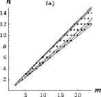
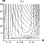
Figure 6: (a) Lattice of quantum numbers on which the part of the spectrum between the “ground state” and the threshold for the entry of the $l=1$ mode is defined, and the unbounded contours of constant eigenvalue. (b) The same, in $\mu\equiv n/m$, $m$ space.

The most unstable modes are those with radial node number $l=0$. Thus we first consider the set $S_{0}\equiv\{\lambda_{0,m,n}|1\leq m\leq m_{\mathrm{max}},m\mu_{\rm min}<n<m\mu_{\rm max}\}$, where $m$ and $n$ are integers and $\mu_{\rm min}$ and $\mu_{\rm max}$ are chosen to give the desired range of $\gamma$. As we shall be rescaling the eigenvalues prior to statistical analysis, it makes no difference whether we work with the spectrum of growth rates $\gamma$ or the eigenvalues $\lambda\equiv-\gamma^{2}$. However the latter choice makes it clearer that the analog of the quantum-mechanical ground state is the most rapidly growing mode—denoting the maximum growth rate of the $l=0$ mode by $\gamma_{0}$, the minimum $\lambda$ is $\lambda_{0}=-\gamma_{\rm max}^{2}=-\gamma_{0}^{2}$.

The spectrum is defined on the fan-like subset of the two-dimensional quantum-number lattice depicted in Fig. 6(a). Also shown are contours of constant $\gamma$ (or $\lambda$), regarded as a continuous function of $m$ and $n$, which are seen more clearly in Fig. 6(b). Here we see a striking contrast with more generic systems Berry and Tabor (1977), where the constant-eigenvalue contours are segments of topological circles enclosing the origin. In the ideal-MHD case the contours are topologically hyperbolic, with asymptotes radiating from the origin toward infinity.

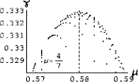
Figure 7: Growth-rate eigenvalues of $l=0$ modes near the maximum growth rate vs. $\mu\equiv n/m$. The ensemble shown is for $m_{\mathrm{max}}=100$.

An interesting representation of the $l=0$ spectrum is shown in Fig. 7. A great deal of structure can be discerned, determined by the number-theoretic properties of the interval of $\mu$ depicted. For instance, focusing on the low-order rational number $4/7$ we define spectral subsets $S_{0}(N/M|4/7)\equiv\{\lambda_{0,m,n}|m=M+7k,n=N+4k,k=0,1,2,\ldots,[(m_{\mathrm{max}}-N)/7]\}$, where $[x]$ denotes the largest integer $\leq x$.

These spectral sequences all accumulate toward the same Suydam eigenvalue $\lambda_{4/7,0}$ as $m_{\mathrm{max}}\rightarrow\infty$ independently of the choice of $M$ and $N$. However the rapidity of this approach is sensitive to the choice of $M/N$. For instance we see in Fig. 7 the most rapidly converging sequence, $S_{0}(4/7|4/7)$, as a set of points accumulating vertically from below toward the Suydam eigenvalue. Other sequences on either side of $S_{0}(4/7|4/7)$ approach the accumulation point obliquely and much more slowly—for $m_{\mathrm{max}}=100$ they visibly have some distance to go. The sequence immediately to the left of $S_{0}(4/7|4/7)$ is $S_{0}(1/2|4/7)$, while that to the right is $S_{0}(3/5|4/7)$, 1/2 and 3/5 being the immediate neighbors of 4/7 in the Farey sequence (Niven et al., 1991, p. 300) of order 7 (the first order at which $4/7$ appears), with the $\mu$-values corresponding to $S_{0}(1/2|4/7)$ and $S_{0}(3/5|4/7)$ providing the immediate neighbors of $4/7$ in each higher-order Farey sequence.

In discussing the structure of the spectrum it is useful to partition $S_{0}$ into two subsets, $S^{-}_{0}$ and $S^{+}_{0}$, according as the points are to the left or right, respectively, of the dashed vertical line shown in Fig. 7 passing through the point of maximum growth rate.

The sequences $S_{0}(1/2|4/7)$ and $S_{0}(3/5|4/7)$ accumulate toward $\lambda_{4/7,0}$, but slower [$O(1/m_{\mathrm{max}})$] than does $S_{0}(4/7|4/7)$ [$O(1/m_{\mathrm{max}}^{2})$, from Sec. III.2.2]. Thus there is a gap containing $\lambda_{4/7,0}$ within which $S_{0}(4/7|4/7)$ contributes $O(m_{\mathrm{max}})$ points to $S^{-}_{0}$, while other sequences contribute at most a set of $O(1)$ points.

Within the gap the spectrum $S^{-}_{0}$ is essentially one-dimensional, being indexed by the single quantum number $k$. In the full spectrum, $S_{0}=S^{-}_{0}\cup S^{+}_{0}$, $O(m_{\mathrm{max}})$ unrelated eigenvalues from $S^{+}_{0}$ appear in the gap, making the spectrum appear more random and two-dimensional.

V Weyl formula

As discussed in Sec. III.2.2, the overall maximum growth rate for the $l=0$ and $1$ modes (and, we assume, for all $l$) occurs at $m=\infty$. Thus the threshold value when a given mode $l$ first starts contributing to the spectrum is at $\lambda=-\gamma_{l}^{2}$, where $\gamma_{l}$ is the maximum over $\mu$ of $\gamma(\mu,l)$. We denote the corresponding value of $\mu$ by $\mu_{l}$.

For fixed $l$ and large $m_{\mathrm{max}}$ the number of eigenvalues $N_{l}(\mu)$ in an interval of $n/m$ between $\mu_{l}$ and $\mu$ is asymptotically equal to the area in the $m,n$ plane [see Fig. 6(a)] of the triangle bounded by the lines $n=\mu m$, $n=\mu_{l}m$ and $m=m_{\mathrm{max}}$. That is, $N_{l}(\mu)\sim{\textstyle{\mathrm{\frac{1}{2}}}}|\mu-\mu_{l}|m_{\mathrm{max}}^{2}$.

Since contours of constant $\lambda$ (or $\gamma$) asymptote to lines of constant $\mu$ as $m\rightarrow\infty$ we can estimate the number of eigenvalues between two values of $\lambda$ (or $\gamma$) by inverting the function $\lambda_{\mu,l}$ for $\mu$ and substituting this into the above expression for $N_{l}(\mu)$. The inverse is double-valued: $\mu=\mu_{l}^{+}(\lambda)>\mu_{l}$ and $\mu_{l}^{-}(\lambda)<\mu_{l}$. Then the number of eigenvalues between the ground state $\lambda_{\mu_{0},l}$ and $\lambda$ is approximately

$$\overline{N}_{l}^{\pm}(\lambda)\equiv{\textstyle{\mathrm{\frac{1}{2}}}}|\mu^{\pm}(\lambda)-\mu_{0}|m_{\mathrm{max}}^{2}\;.$$ (28)

The asymptotic dependence of the total spectrum $S\equiv S_{0}^{-}\cup S_{0}^{+}\cup S_{1}^{-}\cup S_{1}^{+}\cup\ldots$ is thus

$$\overline{N}(\lambda)\equiv\sum_{l=0}^{\infty}\sum_{\pm}\overline{N}_{l}^{\pm}(\lambda)\;.$$ (29)

This is the analog of the Weyl formula (Gutzwiller, 1990, p. 258) for the integral of the smoothed spectral density (“density of states”).

Approximating $\lambda_{\mu,l}=\lambda_{l}+{\textstyle{\mathrm{\frac{1}{2}}}}(\partial^{2}\lambda_{\mu_{l},l}/\partial\mu_{l}^{2})(\mu-\mu_{l})^{2}$ we get $\mu_{l}^{\pm}(\lambda)=\mu_{l}\pm\sqrt{2}(\lambda-\lambda_{l})^{1/2}/(\partial^{2}\lambda_{\mu_{l},l}/\partial\mu_{l}^{2})^{1/2}$. Thus there is a square-root singularity at each mode threshold.

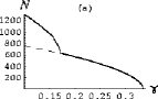
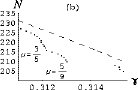
Figure 8: (a) Eigenvalue sequence number $N(\gamma)$ for the combined spectral set $S_{0}\cup S_{1}$ in the case $m_{\mathrm{max}}=100$. The Weyl formula for $S_{0}$, $\overline{N}_{0}^{-}(\gamma)+\overline{N}_{0}^{+}(\gamma)$, is shown dashed. (b) Closeup of region containing eigenvalues associated with $\mu=3/5$ and $\mu=5/9$.

A comparison between the Weyl formula for $S_{0}$ and the set of points $\{(\gamma_{N},N)\}$, where $N$ is the sequence number obtained by sorting the set of $l=0$ and $l=1$ growth-rate eigenvalues from largest to smallest, is shown in Fig. 8(a), showing excellent agreement above the threshold for $S_{1}$. The plotted points may also be regarded as the locations of the steps in the “staircase plot” of the piecewise-constant integrated density of states function $N(\gamma)$, but the scale in this plot is too coarse to resolve the staircase structure.

A finer-scale plot is shown in Fig. 8(b), in which significant deviations from the Weyl curve are seen in the microstructure. The range shown in Fig. 8(b) is unusual in that it contains two well-defined accumulation sequences in close proximity. These are associated with low-order values of $\mu$ occurring on either side of the growth-rate maximum near $\mu=11/19\approx 0.579$—the sequence associated with $\mu=5/9\approx 0.556$ is in $S^{-}_{0}$ and the one associated with $\mu=3/5=0.6$ is in $S^{+}_{0}$. There are very few eigenvalues associated with high-order rational values of $\mu$ in the range shown and the two low-order sequences present are practically unmixed, either with each other or with eigenvalues associated with unrelated higher-order rational values of $\mu$. [In fact there is only one such high-order mode in the region of the accumulation sequences, $\mu=51/92$, the closest approximant to $5/9$ in the set corresponding to $S_{0}(1/2|5/9)$, which causes the slight jump seen in the $\mu=3/5$ sequence.] Also, the wide gap containing no eigenvalues is because the intersection of the gaps associated with the two low-order rationals is non-empty.

The spectrum near the marginal stability point, $\gamma=0$, will involve the superposition of many branches of radial eigenvalue $l$. To estimate the asymptotic behavior of $N(\gamma)$ as $\gamma\rightarrow 0$ we use the approximate dispersion relation Eq. (20). Taking $l$ to be large we see from Eq. (20) that the Suydam growth rates $\gamma_{l}(\mu)$ are sharply peaked about the location of the maximum, $\mu_{0}$, of $G(r_{\mu})$, where $\sigma(\mu)\equiv(G-1/4)^{1/2}$ is also a maximum. Thus we can expand $\sigma(\mu)$ about $\mu_{0}$

$$\sigma(\mu)=\sigma_{\rm max}\left[1-\left(\frac{\mu-\mu_{0}}{\Delta\mu}\right)^{2}\right]+O\left((\mu-\mu_{0})^{3}\right)\;,$$ (30)

where $(\Delta\mu)^{2}\equiv-2\sigma_{\rm max}/\sigma^{\prime\prime}(\mu_{0})$. To leading order all other parameters are evaluated at the maximum point $\mu=\mu_{0}$. The quadratic correction to $\sigma$ need only be retained in the term involving the expansion parameter $l$, so, to leading order,

$$\gamma_{l}\approx\gamma_{0}\exp\left[-\frac{\pi l}{2\sigma(\mu)}\right]\;,$$ (31)

where $\gamma_{0}\equiv 4\dot{{\mbox{$\iota\!\!$-}}}(r_{\mu_{0}})(\sigma_{\rm max}/e)\exp(-\pi/4\sigma_{\rm max}-1/4\sigma_{\rm max}^{2})$.

Solving for $\mu$ we find

$$\mu^{\pm}_{l}(\gamma)=\mu_{0}\pm\Delta\mu\left[1-\frac{l}{l_{\rm max}(\gamma)}\right]^{1/2}\;,$$ (32)

where $l_{\rm max}(\gamma)\equiv(2/\pi)\sigma_{\rm max}\ln(\gamma_{0}/\gamma)$. Substituting Eq. (32) in Eq. (29) and approximating the sum over $l$ by an integral we find the leading order asymptotic behavior of the number of eigenvalues to be

$$\overline{N}(\gamma)\sim\frac{4\Delta\mu}{3\pi}\sigma_{\rm max}m_{\mathrm{max}}^{2}\ln\frac{\gamma_{0}}{\gamma}\;,$$ (33)

which diverges logarithmically as $\gamma\rightarrow 0$.

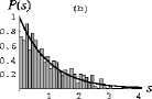
Figure 9: (a) Nearest-neighbor eigenvalue spacing distribution for the approximate spectral set $S_{0}^{\rm Suydam}$ using $\mu_{\rm min}=0.5044$, $\mu_{\rm max}=0.6288$, $m_{\mathrm{max}}=100$ (625 eigenvalues). (b) The same, for the corresponding set of accurate eigenvalues $S_{0}$.

VI Nearest-neighbor statistics

Preparatory to the statistical analysis of eigenvalue spacing it is standard practice to rescale, or unfold, the eigenvalues so as to make their average separation unity, thus making possible the comparison of different systems on the same footing.

We can unfold the spectra by using the Weyl formulae above, e.g. for $\lambda_{i}\in S_{0}^{\pm}$ we can define rescaled eigenvalues $E_{i}^{\pm}$ by

$$E_{i}^{\pm}\equiv\overline{N}_{0}^{\pm}(\lambda_{i})\;.$$ (34)

For the set $S_{0}=S_{0}^{+}\cup S_{0}^{-}$ we can unfold with the combined Weyl function, $\sum_{\pm}\overline{N}_{0}^{\pm}$. However, for practical purposes we have in this section used empirical least-square fits of $N(\gamma)$ to a linear superposition of the basis functions $(\gamma_{\rm max}-\gamma)^{1/2}$, $(\gamma_{\rm max}-\gamma)$, $(\gamma_{\rm max}-\gamma)^{3/2}$, which captures the square-root singularity but avoids having to invert $\gamma_{\mu,l}$.

When $m_{\mathrm{max}}$ is large, the great majority of eigenvalues $\lambda_{l,m,n}$ are very close to the corresponding $m=\infty$ eigenvalue with the same $\mu\equiv n/m$, $\lambda_{\mu,l}$. Thus one might suppose that the statistics of the spectrum are asymptotically the same as those of an ensemble $S_{0}^{\rm Suydam}\equiv\{\lambda_{n/m,0}|1\leq m\leq m_{\mathrm{max}},m\mu_{\rm min}<n<m\mu_{\rm max}\}$.

In Fig. 9(a) we show the distribution of nearest-neighbor unfolded eigenvalue spacings for $S_{0}^{\rm Suydam}$, and in Fig. 9(b) that for the set $S_{0}$ with the correct finite-$m$ eigenvalues. It is seen that the two distributions are radically different—even though low-order rational values of $\mu$ are rare and the distribution is coarse-grained, the high-$m$ approximation induces sufficient extra degeneracy that the Suydam spectrum is dominated by a large, but spurious, delta-function-like spike at $s=0$. (The range of $\mu$ used in Fig. 9 corresponds to the range of $l=0$ growth rates above the maximum $l=1$ rate, in which $S_{0}$ is the only contributor to the spectrum.)

The reason why finite-$m$ effects are so important, despite the smallness of the $O(1/m^{2})$ corrections found in Sec. III.2.2, is seen from the Weyl formula, Eq. (28), which shows that the average eigenvalue spacing in a set containing all values of $n/m$ within the range of interest scales as $m_{\mathrm{max}}^{-2}$, which is the same order as the smallest $O(1/m^{2})$ correction within a set containing only $n/m={\mathrm{const}}$. Thus in the set of accurate eigenvalues $S_{0}$ there is a strong intermingling of eigenvalues with different $n/m$ that does not occur in the approximate set $S_{0}^{\rm Suydam}$.

This explains why the nearest-neighbor eigenvalue spacing distribution in Fig. 9(b) is much closer to the Poisson distribution $\exp(-s)$ obtained for a random distribution of numbers on the real line, and also predicted for generic separable systems Berry and Tabor (1977), than that in Fig. 9(a). Nevertheless the set of $625$ eigenvalues used in Fig. 9(b) is too small to say convincingly that the distribution is or is not Poissonian, so we need to analyze larger data sets to determine how close to generic the ideal-MHD spectrum is.

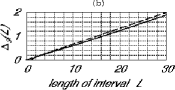
Figure 10: (a) Nearest-neighbor eigenvalue spacing distribution for the spectral set $S_{0}$ using $\mu_{\rm min}=0.5044$, $\mu_{\rm max}=0.6288$, $m_{\mathrm{max}}=1000$ (62,254 eigenvalues). (b) The Dyson-Mehta spectral rigidity for this set (solid line) compared with that for the Poisson process (dashed line).

A cutoff at $m_{\mathrm{max}}=1000$ gives a set $S_{0}$ containing about $62,254$ eigenvalues in the range between the maximum $l=0$ growth rate and the maximum $l=1$ growth rate. [Note the approximately $m_{\mathrm{max}}^{2}$ scaling in the size of $S_{0}$, as predicted by the Weyl formula, Eq. (28).] In Fig. 10(a) we show the nearest-neighbor distribution for this set. Close examination of the region near the origin reveals no trace of the spike seen in Fig. 9(a), not even the tiny spike found by Casati et al. Casati et al. (1985) for the spectrum of waves in an incommensurate rectangular box. However, it is clear that the statistics are not exactly Poissonian.

In Fig. 10(b) we show the Dyson-Mehta rigidity parameter $\Delta_{3}(L)$ (Mehta, 1991, pp. 321–323), defined as the least-squares deviation of the unfolded eigenvalue staircase $N(E)$ from the best-fitting straight line in an interval of length $L$. Again, the behavior is similar to that for the completely random spectrum (Poisson process) in that $\Delta_{3}$ increases linearly with $L$, but the slope is slightly less than the $1/15$ expected for the Poisson processs.

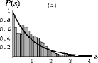
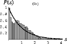
Figure 11: (a) Nearest-neighbor eigenvalue spacing distribution for the spectral set $S_{0}^{-}$ for $m_{\mathrm{max}}=1000$ (37,932 eigenvalues). (b) Nearest-neighbor eigenvalue spacing distribution for the spectral set $S_{0}^{+}$ (24,412 eigenvalues).

In order to understand the departure from Poisson statistics better, we show in Fig. 11 the spacing distribution for the corresponding sets $S_{0}^{-}$ and $S_{0}^{+}$. The departure from Poisson statistics is now quite striking. This is presumably because of the gaps about low-order rational values of $\mu$ mentioned in Sec. IV, which leave the 1-dimensional accumulation sequences $S_{0}(\mu|\mu)$ unmixed with other parts of the spectrum, so the spacing distribution combines aspects of that for a 1-dimensional system (peaked at 1) and that for a generic separable 2-dimensional system (peaked at 0).

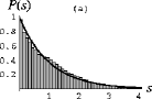
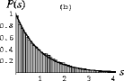
Figure 12: (a) Nearest-neighbor eigenvalue spacing distribution for the first $72,500$ eigenvalues of the $l=1$ spectral set $S_{1}$, $m_{\mathrm{max}}=1000$. (b) Nearest-neighbor eigenvalue spacing distribution for the mixed spectral set $S_{0}\cup S_{1}$ over the same range of eigenvalues as in (a) (total of 95,000 eigenvalues).

In Fig. 12(a) we show the spacing distribution for the $l=1$ spectrum, which is seen to be very much like the $l=0$ spectrum of Fig. 10(a) in its departure from the Poisson distribution. However, we might expect that mixing the $l=0$ with the $l=1$ spectrum will make the levels appear more “random” and Fig. 12(b) confirms that the level spacing distribution does indeed become more like the exponential expected for a Poisson process.

VII Conclusion

We have demonstrated that the statistical nature of the ideal-MHD interchange spectrum deviates significantly from the random Poisson process of generic separable systems due to the number-theoretic structure of the eigenvalue distribution. The similarity between the two level-spacing distributions in Fig. 11, which correspond to two different parts of the rotational transform profile, suggest the possibility that there may nevertheless be some universality in the statistics. If so, we have found a new universality class.

The crude regularization used in this paper, simply restricting the poloidal mode numbers to $m\leq m_{\mathrm{max}}$, is not very physical but corresponds closely to what is done in the large three-dimensional eigenvalue codes CAS3D Schwab (1993) and TERPSICHORE Anderson et al. (1990). Thus, apart from fundamental mathematical interest, the primary motivation of this paper has been the numerical analysis of the three-dimensional ideal-MHD spectrum as produced by these codes. Preliminary results Dewar et al. (2004) on an interchange-unstable stellarator test case show spectra with eigenvalue separation statistics similar to those of strongly quantum chaotic systems. However, the results of the present paper indicate that some caution should be taken in interpreting ideal-MHD spectra in terms of conventional quantum chaos theory because of the radically different nature of the dispersion relation.

In subsequent work it will be important to examine the effect of finite Larmor radius on the spectrum. However, this typically makes the problem non-Hermitian and less easy to compare with standard quantum chaos theory.

Appendix A $1/m^{2}$ Corrections

The coefficients of the expansion Eq. (14) are found by Taylor expansion of the geometric and equilibrium quantities in Eqs. (5)

$$L^{(0)} = -\frac{d}{dx}\dot{{\mbox{$\iota\!\!$-}}}^{2}x^{2}\frac{d}{dx}+\dot{{\mbox{$\iota\!\!$-}}}^{2}x^{2}-D_{\mathrm{S}}\;,$$

$$L^{(1)} = x\frac{d}{dx}\dot{{\mbox{$\iota\!\!$-}}}^{2}x^{2}\frac{d}{dx}-\frac{d}{dx}\dot{{\mbox{$\iota\!\!$-}}}\,\ddot{{\mbox{$\iota\!\!$-}}}\,x^{3}\frac{d}{dx}$$

$$\mbox{}+\dot{{\mbox{$\iota\!\!$-}}}\,(\ddot{{\mbox{$\iota\!\!$-}}}-3\,\dot{{\mbox{$\iota\!\!$-}}})x^{3}+(2D_{\mathrm{S}}-\dot{D}_{\mathrm{S}}-\dot{{\mbox{$\iota\!\!$-}}}\,\ddot{{\mbox{$\iota\!\!$-}}})x\;,$$

$$L^{(2)} = -x^{2}\frac{d}{dx}\dot{{\mbox{$\iota\!\!$-}}}^{2}x^{2}\frac{d}{dx}+x\frac{d}{dx}\dot{{\mbox{$\iota\!\!$-}}}\,\ddot{{\mbox{$\iota\!\!$-}}}\,x^{3}\frac{d}{dx}$$ (35)

$$\mbox{}+\frac{d}{dx}x^{4}\left(\frac{\dot{{\mbox{$\iota\!\!$-}}}^{2}}{12}-\frac{\ddot{{\mbox{$\iota\!\!$-}}}^{2}}{4}+\frac{\dot{{\mbox{$\iota\!\!$-}}}\,\ddot{{\mbox{$\iota\!\!$-}}}}{2}-\frac{\dot{{\mbox{$\iota\!\!$-}}}\,\dddot{{\mbox{$\iota\!\!$-}}}}{3}\right)\frac{d}{dx}$$

$$\mbox{}+\frac{x^{2}}{2}\left(5\,\dot{{\mbox{$\iota\!\!$-}}}\,\ddot{{\mbox{$\iota\!\!$-}}}-2\,\dot{{\mbox{$\iota\!\!$-}}}\,\dddot{{\mbox{$\iota\!\!$-}}}-\ddot{{\mbox{$\iota\!\!$-}}}^{2}-6D_{\mathrm{S}}+5\dot{D}_{\mathrm{S}}-\ddot{D}_{\mathrm{S}}\right)$$

$$\mbox{}+x^{4}\left(\frac{71\,\dot{{\mbox{$\iota\!\!$-}}}^{2}}{12}+\frac{\ddot{{\mbox{$\iota\!\!$-}}}^{2}}{4}-\frac{7\,\dot{{\mbox{$\iota\!\!$-}}}\,\ddot{{\mbox{$\iota\!\!$-}}}}{2}+\frac{\dot{{\mbox{$\iota\!\!$-}}}\,\dddot{{\mbox{$\iota\!\!$-}}}}{3}\right)$$

and (8)

$$M^{(0)} = -\frac{d^{2}}{dx^{2}}+1\;,$$

$$M^{(1)} = x\frac{d^{2}}{dx^{2}}-\frac{d}{dx}x\frac{d}{dx}-2x\;,$$

$$M^{(2)} = -x^{2}\frac{d^{2}}{dx^{2}}+x\frac{d}{dx}x\frac{d}{dx}+3x^{2}\;.$$ (36)

where, as in the main text, dots denote nondimensional derivatives, $\dot{{\mbox{$\iota\!\!$-}}}\equiv r_{\mu}d\iota/dr$ etc., and all equilibrium quantities are evaluated at $r=r_{\mu}$.

References

- Casati et al. (1985) G. Casati, B. V. Chirikov, and I. Guarneri, Phys. Rev. Letters 54, 1350 (1985).
- Wakatani (1998) M. Wakatani, Stellarator and Heliotron Devices, no. 95 in The international series of monographs on physics (Oxford University Press, New York, 1998).
- Lifschitz (1989) A. E. Lifschitz, Magnetohydrodynamics and Spectral Theory (Kluwer, Dordrecht, The Netherlands, 1989).
- Spies and Tataronis (2003) G. O. Spies and J. A. Tataronis, Phys. Plasmas 10, 413 (2003).
- Hameiri (1985) E. Hameiri, Commun. Pure Appl. Math. 38, 43 (1985).
- Troyon et al. (1984) F. Troyon, R. Gruber, H. Saurenmann, S. Semenzato, and S. Succi, Plasma Phys. 26, 209 (1984).
- Ferron et al. (2000) J. R. Ferron, M. S. Chu, G. L. Jackson, L. L. Lao, R. L. Miller, T. H. Osborne, P. B. Snyder, E. J. Strait, T. S. Taylor, A. D. Turnbull, et al., Phys. Plasmas 7, 1976 (2000).
- Anderson et al. (1990) D. V. Anderson, W. A. Cooper, R. Gruber, S. Merazzi, and U. Schwenn, Int. J. Supercomp. Appl. 4, 34 (1990).
- Schwab (1993) C. Schwab, Phys. Fluids B 5, 3195 (1993).
- Bernstein et al. (1958) I. B. Bernstein, E. A. Frieman, M. D. Kruskal, and R. M. Kulsrud, Proc. R. Soc. London Ser. A 244, 17 (1958).
- Dewar and Glasser (1983) R. L. Dewar and A. H. Glasser, Phys. Fluids 26, 3038 (1983).
- Cuthbert et al. (1998) P. Cuthbert, J. L. V. Lewandowski, H. J. Gardner, M. Persson, D. B. Singleton, R. L. Dewar, N. Nakajima, and W. A. Cooper, Phys. Plasmas 5, 2921 (1998).
- Redi et al. (2002) M. H. Redi, J. L. Johnson, S. Klasky, J. Canik, R. L. Dewar, and W. A. Cooper, Phys. Plasmas 9, 1990 (2002).
- Gutzwiller (1990) M. C. Gutzwiller, Chaos in Classical and Quantum Mechanics, no. 1 in Interdisciplinary Applied Mathematics Series (Springer-Verlag, New York, 1990).
- Stöckmann (1999) H. J. Stöckmann, Quantum Chaos: An Introduction (Cambridge University Press, Cambridge, 1999).
- Haake (2001) F. Haake, Quantum Signatures of Chaos (Springer-Verlag, Berlin, 2001), 2nd ed.
- Mehta (1991) M. L. Mehta, Random Matrices (Academic Press, San Diego, 1991), 2nd ed.
- Dewar et al. (2001) R. L. Dewar, P. Cuthbert, and R. Ball, Phys. Rev. Letters 86, 2321 (2001), arXiv:physics/0102065.
- Berry and Tabor (1977) M. V. Berry and M. Tabor, Proc. R. Soc. Lond. A 356, 375 (1977).
- Suydam (1958) B. R. Suydam, in Proc. Second Int. Conf. on the Peaceful Uses of Atomic Energy (United Nations, Geneva, 1958), vol. 31, p. 157.