Abstract

A review of methods for finding general expressions for matrix elements (non-diagonal with respect to configurations included) of any one- and two-particle operator for an arbitrary number of shells in an atomic configuration is given. These methods are compared in various aspects, and the advantages or shortcomings of each particular method are discussed. Efficient method to find the abovementioned quantities in $LS$ coupling is presented, based on the use of symmetry properties of operators and matrix elements in three spaces (orbital, spin and quasispin), second quantization in coupled tensorial form, graphical technique and Wick’s theorem. This allows to efficiently account for correlation effects practically for any atom and ion of periodical table.

PACS: 0270, 3110, 3115

1 Introduction

Modern atomic spectroscopy studies the structure and properties of practically any atom of the periodic table as well as of ions of any ionization degree. Particular attention is paid to their energy spectra. For the investigations of many-electron atoms and ions, it is of great importance to combine experimental and theoretical methods. Nowadays the possibilities of theoretical spectroscopy are much enlarged thanks to the wide use of powerful computers. Theoretical methods utilized must be fairly universal and must ensure reasonably accurate values of physical quantities studied.

Many-electron atom usually is considered as many-body problem and is described by the wave function constructed from the wave functions of one electron, moving in the central nuclear charge field and in the screening field of the remaining electrons. Then the wave function of this electron may be represented as a product of radial and spin-angular parts. The radial part is usually found by solving various modifications of the Hartree-Fock equations and can be represented in a numerical or analytical forms (Froese Fischer [1]) whereas the angular part is expressed in terms of spherical functions. Then the wave function of the whole atom can be constructed in some standard way (Cowan [2], Jucys and Savukynas [3], Nikitin and Rudzikas [4]) starting with these one-electron functions and may be used further on for the calculations of any matrix elements representing physical quantities.

For obtaining the values of atomic quantities it is necessary to solve so-called eigenvalue problem

$$H\Psi=E\Psi,$$ (1)

where $\Psi$ is the wave function of the system under investigation and $H$ is its Hamiltonian. In order to obtain accurate values of atomic quantities it is necessary to account for relativistic and correlation effects. It turned out that for very large variety of atoms and their ionization degrees the relativistic effects may be taken into account fairly accurately as Breit-Pauli corrections (Nikitin and Rudzikas [4], Rudzikas [5]). It is convenient to present the Hamiltonian as consisting of two parts in Breit-Pauli approach, namely,

$$H_{BP}=H_{NR}+H_{R},$$ (2)

where $H_{NR}$ is the non-relativistic Hamiltonian and $H_{R}$ stands for the relativistic contibution. Non-relativistic Hamiltonian is the sum of the kinetic energy of electrons $T$, their potential energy $P$, and the electrostatic electron interaction $Q$

$$H_{NR}=T+P+Q.$$ (3)

The first two terms, $T$ and $P$ are the one-particle operators, whereas the third term, $Q$, is two-particle operator. The $H_{R}$ may also be subdivided into non-fine structure and fine structure contributions

$$H_{R}=H_{Non-Fine}+H_{Fine}.$$ (4)

The non-fine structure contributions

$$H_{Non-Fine}=H_{Mass}+H_{D1}+H_{D2}+H_{SSC}+H_{OO}$$ (5)

shift non-relativistic energy levels without any splitting of them. The mass-velocity term $H_{Mass}$ describes the variation of mass with velocity. The one- and two-body Darwin (contact) terms $H_{D1}$ and $H_{D2}$ are the corrections of the one-electron Dirac equation due to the retardation of the electromagnetic field produced by an electron (contact interaction). The spin-spin-contact term $H_{SSC}$ accounts for the interaction of the spin magnetic moments of two electrons occupying the same space. The orbit-orbit interaction $H_{OO}$ accounts for the interaction of two orbital moments.

The fine-structure contributions

$$H_{Fine}=H_{SO}+H_{SOO}+H_{SS}$$ (6)

split the non-relativistic energy levels (terms) into a series of closely-spaced levels. The most important of these is the nuclear spin-orbit interaction $H_{SO}$ (spin-own-orbit) representing the interaction of the spin and angular magnetic moments of an electron in the field of the nucleus. The spin-other-orbit $H_{SOO}$ and spin-spin $H_{SS}$ contributions in a rough sense may be viewed as corrections to the nuclear spin-orbit interaction due to the presence of the other electrons in the system.

Unfortunately, practical calculations show that all realistic atomic Hamiltonians do not lead straightforwardly to eigenvalue problem (1). Actually we have to calculate all non-zero matrix elements of the Hamiltonian considered including those non-diagonal with respect to electronic configurations, then to form energy matrix, to diagonalize it, obtaining in this way the values of the energy levels as well as the eigenfunctions (the wave functions in the intermediate coupling scheme). The latter may be used then to calculate electronic transitions as well as the other properties and processes. Such a necessity raises special requirements for the theory.

The total matrix element of each term of the energy operator in the case of complex electronic configuration will consist of matrix elements, describing the interaction inside each shell of equivalent electrons as well as between these shells. Going beyond the single-configuration approximation we have to be able to take into account in the same way non-diagonal, with respect to configurations, matrix elements.

To find the expressions for the matrix elements of all terms of the Hamiltonian considered for complex electronic configurations, having several open shells, is a task very far from the trivial one. A considerable part of the effort must be devoted to coping with integrations over spin-angular variables, occurring in the matrix elements of the operators under consideration. This paper presents the general methodology, leading to optimal expressions for operators and matrix elements.

A number of methodologies to calculate the angular parts of matrix elements exists in literature. Many existing codes for integrating the spin-angular parts of matrix elements (Glass [6], Glass and Hibbert [7], Grant [8], Burke et al  [9]) are based on the computational scheme proposed by Fano [10]. This methodology is based on having the total wavefunction of an atom built from the antisymmetrized wavefunctions of separate shells, and this antisymmetrization is done via coefficients of fractional parentage. The shells are coupled one to another via their angular momenta. So, the finding of matrix elements amounts to finding the recoupling matrices and the coefficients of fractional parentage.

Suppose that we have a bra function with $u$ shells in $LS$ coupling:

$$\begin{array}[b]{c}\psi_{u}^{bra}\left(LSM_{L}M_{S}\right)\equiv\\ \equiv(n_{1}l_{1}n_{2}l_{2}...n_{u}l_{u}\alpha_{1}L_{1}S_{1}\alpha_{2}L_{2}S_{2}...\alpha_{u}L_{u}S_{u}{\cal A}LSM_{L}M_{S}|\end{array}$$ (7)

and a ket function:

$$\begin{array}[b]{c}\psi_{u}^{ket}\left(L^{\prime}S^{\prime}M^{\prime}_{L}M^{\prime}_{S}\right)\equiv\\ \equiv|n_{1}l_{1}n_{2}l_{2}...n_{u}l_{u}\alpha_{1}^{\prime}L_{1}^{\prime}S_{1}^{\prime}\alpha_{2}^{\prime}L_{2}^{\prime}S_{2}^{\prime}...\alpha_{u}^{\prime}L_{u}^{\prime}S_{u}^{\prime}{\cal A}^{\prime}L^{\prime}S^{\prime}M^{\prime}_{L}M^{\prime}_{S}),\end{array}$$ (8)

where ${\cal A}$ stands for all intermediate quantum numbers, depending on the order of coupling of momenta $L_{i}S_{i}$. Using the Wigner-Eckart theorem in $LS$ space we shift from the matrix element of any two-particle operator $\widehat{G}$ between functions (7) and (8) to the submatrix element (reduced matrix)

$(\psi_{u}^{bra}\left(LS\right)||\widehat{G}^{\left(\kappa_{1}\kappa_{2}k,\sigma_{1}\sigma_{2}k\right)}||\psi_{u}^{ket}\left(L^{\prime}S^{\prime}\right))$ of this operator. When the two-particle operator acts upon four distinct shells, then the finding general expressions of matrix elements, according to methodology by Fano [10], is based upon the formula

$$\begin{array}[b]{c}(\psi_{u}^{bra}\left(LS\right)||\widehat{G}^{\left(\kappa_{1}\kappa_{2}k,\sigma_{1}\sigma_{2}k\right)}||\psi_{u}^{ket}\left(L^{\prime}S^{\prime}\right))\sim\\ \sim\displaystyle{\sum_{n_{i}\lambda_{i},n_{j}\lambda_{j},n_{i^{\prime}}\lambda_{i^{\prime}},n_{j^{\prime}}\lambda_{j^{\prime}}}}\left(-1\right)^{\Delta}\left[N_{i}\left(N_{j}-\delta(i,j)\right)N_{i^{\prime}}^{\prime}\left(N_{j^{\prime}}^{\prime}-\delta(i^{\prime},j^{\prime})\right)\right]^{1/2}\times\\ \times\left(l_{i}^{N_{i}}\;\alpha_{i}L_{i}S_{i}||l_{i}^{N_{i}-1}\;\left(\alpha_{i}^{\prime}L^{\prime}_{i}S^{\prime}_{i}\right),l_{i}\right)\left(l_{j}^{N_{j}}\;\alpha_{j}L_{j}S_{j}||l_{j}^{N_{j}-1}\;\left(\alpha_{j}^{\prime}L^{\prime}_{j}S^{\prime}_{j}\right),l_{j}\right)\times\\ \times\left(l_{i^{\prime}}^{N_{i^{\prime}}}\;\alpha_{i^{\prime}}L_{i^{\prime}}S_{i^{\prime}}||l_{i^{\prime}}^{N_{i^{\prime}}-1}\;\left(\alpha_{i^{\prime}}^{\prime}L^{\prime}_{i^{\prime}}S^{\prime}_{i^{\prime}}\right),l_{i^{\prime}}\right)\left(l_{j^{\prime}}^{N_{j^{\prime}}}\;\alpha_{j^{\prime}}L_{j^{\prime}}S_{j^{\prime}}||l_{j^{\prime}}^{N_{j^{\prime}}-1}\;\left(\alpha_{j^{\prime}}^{\prime}L^{\prime}_{j^{\prime}}S^{\prime}_{j^{\prime}}\right),l_{j^{\prime}}\right)\times\\ \times\left\{R_{d}\left(\lambda_{i},\lambda_{j},\lambda_{i}^{\prime},\lambda_{j}^{\prime},\kappa_{1},\kappa_{2},\kappa,\sigma_{1},\sigma_{2},\sigma,\Lambda^{bra},\Lambda^{ket}\right)\right.\\ \times\left(1+\delta(i,j)\delta(i^{\prime},j^{\prime})\right)^{-1}\left(n_{i}\lambda_{i}n_{j}\lambda_{j}||g^{\left(\kappa_{1}\kappa_{2}k,\sigma_{1}\sigma_{2}k\right)}||n_{i}^{\prime}\lambda_{i}^{\prime}n_{j}^{\prime}\lambda_{j}^{\prime}\right)-\\ -R_{e}\left(\lambda_{i},\lambda_{j},\lambda_{i}^{\prime},\lambda_{j}^{\prime},\kappa_{1},\kappa_{2},\kappa,\sigma_{1},\sigma_{2},\sigma,\Lambda^{bra},\Lambda^{ket}\right)\\ \times\left.\left(1+\delta(i,j))(1-\delta(i^{\prime},j^{\prime})\right)\left(n_{i}\lambda_{i}n_{j}\lambda_{j}||g^{\left(\kappa_{1}\kappa_{2}k,\sigma_{1}\sigma_{2}k\right)}||n_{j}^{\prime}\lambda_{j}^{\prime}n_{i}^{\prime}\lambda_{i}^{\prime}\right)\right\},\end{array}$$ (9)

where $\Delta$ is a phase factor, (see for example in [8]),

$\Lambda^{bra}\equiv\left(L_{i}S_{i},L_{j}S_{j},L_{i}^{\prime}S_{i}^{\prime},L_{j}^{\prime}S_{j}^{\prime}\right)^{bra}$ is the array for the bra function shells’ terms, and similarly for $\Lambda^{ket}$. The coefficient $\left(l^{N}\;\alpha LS||l^{N-1}\;\left(\alpha^{\prime}L^{\prime}S^{\prime}\right)l\right)$ is a fractional parentage coefficient, and coefficients

$R_{d}\left(\lambda_{i},\lambda_{j},\lambda_{i}^{\prime},\lambda_{j}^{\prime},\kappa_{1},\kappa_{2},\kappa,\sigma_{1},\sigma_{2},\sigma,\Lambda^{bra},\Lambda^{ket}\right)$ and

$R_{e}\left(\lambda_{i},\lambda_{j},\lambda_{i}^{\prime},\lambda_{j}^{\prime},\kappa_{1},\kappa_{2},\kappa,\sigma_{1},\sigma_{2},\sigma,\Lambda^{bra},\Lambda^{ket}\right)$ are the recoupling matrices in $l$ and $s$ - spaces of direct and exchange terms, respectively. For more detailes on recoupling matrices see in Grant [8], Burke et al  [9].

The summation in expression (9) implies that the quantum numbers $n$, $\lambda$ of all participating shells are included. There are four such pairs of $n$, $\lambda$ in the sum.

In essence, the Fano calculation scheme consists of evaluating recoupling matrices. Although such an approach uses classical Racah algebra [11, 12, 13, 14] on the level of coefficients of fractional parentage, it may be necessary to carry out multiple summations over intermediate terms. Due to these summations and the complexity of the recoupling matrix itself, the associated computer codes become rather time consuming. Jucys and Vizbaraitė [15] proposed to use the two-electron coefficients of fractioanl parentage instead of ordinary ones, in matrix elements’ calculations, but even that did not solve the abovementioned problems. A solution to this problem was found by Burke et al  [9]. They tabulated separate standard parts of recoupling matrices along with coefficients of fractional parentage at the beginning of a calculation and used them further on to calculate the needed coefficients. Computer codes by Glass [6], Glass and Hibbert [7], Grant [8], Burke et al  [9] utilize the program NJSYM (Burke [16]) or NJGRAF (Bar-Shalom and Klapisch [17]) for the calculation of recoupling matrices. Both are rather time consuming when calculating matrix elements of complex operators or electronic configurations with many open shells.

In order to simplify the calculations, Cowan [2] suggested that matrix elements be grouped into ”Classes” (see Cowan [2] Figure 13-5). Unfortunately, this approach was not generalized to all two-electron operators. Perhaps for this reason Cowan’s approach is not very popular although the program itself, based on this approach, is widely used.

Many approaches for the calculation of spin-angular coefficients (Glass [6], Glass and Hibbert [7], Grant [8], Burke et al  [9]) are based on the usage of Racah algebra only on the level of coefficients of fractional parentage. A few authors (Jucys and Savukynas [3], Cowan [2]) utilize the unit tensors, simplifying the calculations in this way, because use can be made of the tables of unit tensors and selection rules can be used prior to computation to check whether the spin-angular coefficients are zero or not. Moreover, the recoupling matrices themselves have a simpler form. Unfortunately, these ideas were applied only to diagonal matrix elements with respect to configurations, though Cowan [2] suggested the usage of unit tensors for non-diagonal ones as well.

All the above mentioned approaches were applied in the coordinate representation. The second quantization formalism (Judd [18, 19], Rudzikas and Kaniauskas [20] and Rudzikas [5]) has a number of advantages compared to coordinate representation. First of all, it is much easier to find algebraic expressions for complex operators and their matrix elements, when relying on second quantization formalism. It has contributed significantly to the successful development of perturbation theory (see Lindgren and Morrison [21], Merkelis et al [22], and orthogonal operators (Uylings [23]), where three-particle operators already occur. Uylings [24] suggested a fairly simple approach for dealing with separate cases of three-particle operators.

Moreover, in the second quantization approach the quasispin formalism was efficiently developed by Innes [25], Špakauskas et al [26, 27], Rudzikas and Kaniauskas [20], Fano and Rau [28]. The main advantage of this approach is that applying the quasispin method for calculating the matrix elements of any operator, we can use all advantages of the new version of Racah algebra (see Rudzikas [5]) for integration of spin-angular part of any one- and two-particle operator. For example, the reduced coefficients of fractional parentage are independent of the occupation number of the shell (see Rudzikas and Kaniauskas [20], Gaigalas et al [29]). All this enabled Merkelis and Gaigalas [30] to work out a general perturbation theory approach for complex cases of several open shells. In the paper by Merkelis [31] a detailed review of a version of graphical methodology is presented that allows one to represent the operators graphically and to find the matrix elements of these operators using diagrammatic technique.

The majority of methods and computer codes of finding angular coefficients discussed above were faced with a number of problems, the main of these being:

• The high demand of CPU time for calculating the angular parts of matrix elements even on the modern computer. Therefore the high accuracy of characteristics of atomic quantities somtimes is even unattainable.

• The methods are applicable in practice only for the comparatively simple systems, because in the programs based on classical Racah algebra the treatment of recoupling matrices is rather complicated, especialy when finding the matrix elements of Breit-Pauli operators between complex configurations.

• The configurations with open $f$-shells must often be included in theoretical calculations. This causes problems in a number of methodologies, because the complete account of $f$- shells implies using a large number of coefficients of fractional parentage.

Gaigalas and Rudzikas [32], Gaigalas et al [33], Gaigalas et al [34], Gaigalas et al [29] and Gaigalas and Rudzikas [35] suggested an efficient and general approach for finding the spin-angular parts of matrix elements of atomic interactions, relying on the combination of the second-quantization approach in the coupled tensorial form, the generalized graphical technique and angular momentum theory in orbital, spin and quasispin spaces as well as on the symetry properties of the quantities considered. This approach is free of previous shortcomings.

It is the main goal of this work to present all this methodology consistently and in a unifying manner, paying the special attention to its main ideas. Also, we aim at a detailed discussion of obtaining the efficient tensorial expressions of a two-particle operator, as well as the analytical expressions for recoupling matrices. In addition to that, in this work we aim at comparing this methodology to other calculation of angular coefficients schemes.

From what is said above we see that the treatment of angular parts of matrix elements is a many-sided question. The classical scheme by Fano was developed in various aspects. The methods were developed that used Racah algebra [11, 12, 13, 14] on a higher level, or used the new version of the Racah algebra (angular momentum theory in orbital, spin and quasispin spaces) (see Rudzikas [36]). The ways were searched for, to obtain the expressions that had simpler recoupling matrices. In order to discuss all that in more detail, to compare the existing methods of obtaining the angular parts and to mark the advantages of one method or another, the finding angular parts must be looked at from different angles.

Thus, the first thing to discuss is the expression for any physical operator (see sections 2,3,4), because already the form of it determines the level of application of tensor algebra in the calculation of matrix elements of this operator. Also, it is very important to make clear to what extent the Racah algebra is exploited in one or another methodology of angular parts treatment. This helps to mark the advantages of one method against another (see section 5). In addition, it is of importance to compare the ways of calculating the recoupling matrix in various methods (see section 6).

2 Tensorial Expressions for Two-particle Operators

It is well known in the literature that a scalar two-particle operator may be presented the following tensorial form (see Jucys and Savukynas [3], Glass [6]):

$$\widehat{G}^{\left(\kappa_{1}\kappa_{2}k,\sigma_{1}\sigma_{2}k\right)}=\displaystyle{\sum_{i>j}}g\left(r_{i},r_{j}\right)\displaystyle{\sum_{p}}\left(-1\right)^{k-p}\left[\widehat{g}_{i}^{\left(\kappa_{1}\sigma_{1}\right)}\times\widehat{g}_{j}^{\left(\kappa_{2}\sigma_{2}\right)}\right]_{p-p}^{(k~{}k)},$$ (10)

where $g\left(r_{i},r_{j}\right)$ is the radial part of operator, $\widehat{g}_{i}^{\left(\kappa_{1}\sigma_{1}\right)}$ is a tensor acting upon the orbital and spin variables of the $i$-th function, $\kappa_{1}$, $\kappa_{2}$ are the ranks of operator acting in orbital space, and $\sigma_{1}$, $\sigma_{2}$ are the ranks of operator acting in spin space.

All the above mentioned approaches were usually applied in the coordinate representation. Now we will investigate into the second quantization formalism, which is broadly applied in atomic physics as well.

A two-particle operator in second quantization method is written as follows:

$$G^{\left(\kappa_{1}\kappa_{2}k,\sigma_{1}\sigma_{2}k\right)}=\displaystyle{\sum_{n_{i}l_{i},n_{j}l_{j},n_{i^{\prime}}l_{i^{\prime}},n_{j^{\prime}}l_{j^{\prime}}}}\widehat{G}(ij,i^{\prime}j^{\prime})=\frac{1}{2}\displaystyle{\sum_{i,j,i^{\prime},j^{\prime}}}a_{i}a_{j}a_{j^{\prime}}^{\dagger}a_{i^{\prime}}^{\dagger}\left(i,j|g|i^{\prime},j^{\prime}\right),$$ (11)

where $i\equiv n_{i}l_{i}sm_{l_{i}}m_{s_{i}}$, $\left(i,j|g|i^{\prime},j^{\prime}\right)$ is the two-electron matrix element of operator $G^{\left(\kappa_{1}\kappa_{2}k,\sigma_{1}\sigma_{2}k\right)}$, and $a_{i}$ is the electron creation and $a_{j}^{\dagger}$ electron annihilation operators. Meanwhile two tensorial forms are well known in second quantization. In the first form the operators of second quantization follow in the normal order:

$$\begin{array}[b]{c}G_{I}^{\left(\kappa_{1}\kappa_{2}k,\sigma_{1}\sigma_{2}k\right)}=\displaystyle{\sum_{n_{i}l_{i},n_{j}l_{j},n_{i}^{\prime}l_{i}^{\prime},n_{j}^{\prime}l_{j}^{\prime}}}\widehat{G}_{I}(ij,i^{\prime}j^{\prime})=\\ =-\frac{1}{2}\displaystyle{\sum_{n_{i}l_{i},n_{j}l_{j},n_{i}^{\prime}l_{i}^{\prime},n_{j}^{\prime}l_{j}^{\prime}}}\displaystyle{\sum_{\kappa_{12}\kappa_{12}^{{}^{\prime}}\sigma_{12}\sigma_{12}^{{}^{\prime}}}}\displaystyle{\sum_{p}}\left(-1\right)^{k-p}\left[\kappa_{12},\kappa_{12}^{\prime},\sigma_{12},\sigma_{12}^{\prime}\right]^{1/2}\times\\ \times\left(n_{i}\lambda_{i}n_{j}\lambda_{j}||g^{\left(\kappa_{1}\kappa_{2}k,\sigma_{1}\sigma_{2}k\right)}||n_{i}^{\prime}\lambda_{i}^{\prime}n_{j}^{\prime}\lambda_{j}^{\prime}\right)\times\\ \times\left\{\begin{array}[]{ccc}l_{i}^{\prime}&l_{j}^{\prime}&\kappa_{12}^{\prime}\\ \kappa_{1}&\kappa_{2}&k\\ l_{i}&l_{j}&\kappa_{12}\end{array}\right\}\left\{\begin{array}[]{ccc}s&s&\sigma_{12}^{\prime}\\ \sigma_{1}&\sigma_{2}&k\\ s&s&\sigma_{12}\end{array}\right\}\times\\ \times\left[\left[a^{\left(\lambda_{i}\right)}\times a^{\left(\lambda_{j}\right)}\right]^{\left(\kappa_{12}\sigma_{12}\right)}\times\left[\stackrel{{\scriptstyle\sim}}{{a}}^{\left(\lambda_{i}^{\prime}\right)}\times\stackrel{{\scriptstyle\sim}}{{a}}^{\left(\lambda_{j}^{\prime}\right)}\right]^{\left(\kappa_{12}^{\prime}\sigma_{12}^{\prime}\right)}\right]_{p-p}^{\left(kk\right)},\end{array}$$ (12)

where $\left[a,b\right]=\left(2a+1\right)\left(2b+1\right)$, $\lambda\equiv ls$, $\left(n_{i}\lambda_{i}n_{j}\lambda_{j}||g^{\left(\kappa_{1}\kappa_{2}k,\sigma_{1}\sigma_{2}k\right)}||n_{i}^{\prime}\lambda_{i}^{\prime}n_{j}^{\prime}\lambda_{j}^{\prime}\right)$ is the two-electron submatrix (reduced matrix) element of operator $G^{\left(\kappa_{1}\kappa_{2}\kappa,\sigma_{1}\sigma_{2}\sigma\right)}$ and tensor $\stackrel{{\scriptstyle\sim}}{{a}}^{\left(\lambda\right)}$ is defined as (see for example Rudzikas [5])

$$\stackrel{{\scriptstyle\sim}}{{a}}_{m_{\lambda}}^{\left(\lambda\right)}=\left(-1\right)^{\lambda-m_{\lambda}}a_{-m_{\lambda}}^{\dagger\left(\lambda\right)}.$$ (13)

The product of tensors $\left[\left[a^{\left(\lambda_{i}\right)}\times a^{\left(\lambda_{j}\right)}\right]^{\left(\kappa_{12}\sigma_{12}\right)}\times\left[\stackrel{{\scriptstyle\sim}}{{a}}^{\left(\lambda_{i}^{\prime}\right)}\times\stackrel{{\scriptstyle\sim}}{{a}}^{\left(\lambda_{j}^{\prime}\right)}\right]^{\left(\kappa_{12}^{\prime}\sigma_{12}^{\prime}\right)}\right]_{p-p}^{\left(kk\right)}$ denotes tensorial part of operator $G_{I}^{\left(\kappa_{1}\kappa_{2}k,\sigma_{1}\sigma_{2}k\right)}$.

In another form the second quantization operators are coupled by pairs consisting of electron creation and annihilation operators. In coupled tensorial form:

$$\begin{array}[b]{c}G_{II}^{\left(\kappa_{1}\kappa_{2}\kappa,\sigma_{1}\sigma_{2}\sigma\right)}=\displaystyle{\sum_{n_{i}l_{i},n_{j}l_{j},n_{i}^{\prime}l_{i}^{\prime},n_{j}^{\prime}l_{j}^{\prime}}}\widehat{G}_{II}(ij,i^{\prime}j^{\prime})=\\ =\frac{1}{2}\displaystyle{\sum_{n_{i}l_{i},n_{j}l_{j},n_{i}^{\prime}l_{i}^{\prime},n_{j}^{\prime}l_{j}^{\prime}}}\displaystyle{\sum_{p}}\left(-1\right)^{k-p}\left(n_{i}\lambda_{i}n_{j}\lambda_{j}||g^{\left(\kappa_{1}\kappa_{2}k,\sigma_{1}\sigma_{2}k\right)}||n_{i}^{\prime}\lambda_{i}^{\prime}n_{j}^{\prime}\lambda_{j}^{\prime}\right)\times\\ \times\left\{\left[\kappa_{1},\kappa_{2},\sigma_{1},\sigma_{2}\right]^{-1/2}\times\left[\left[a^{\left(\lambda_{i}\right)}\times\stackrel{{\scriptstyle\sim}}{{a}}^{\left(\lambda_{i}^{\prime}\right)}\right]^{\left(\kappa_{1}\sigma_{1}\right)}\times\left[a^{\left(\lambda_{j}\right)}\times\stackrel{{\scriptstyle\sim}}{{a}}^{\left(\lambda_{j}^{\prime}\right)}\right]^{\left(\kappa_{2}\sigma_{2}\right)}\right]_{p-p}^{\left(kk\right)}-\right.\\ \left.-\left(-1\right)^{l_{i}+l_{j}^{\prime}}\left\{\begin{array}[]{ccc}\kappa_{1}&\kappa_{2}&k\\ l_{j}^{\prime}&l_{i}&l_{j}\end{array}\right\}\left\{\begin{array}[]{ccc}\sigma_{1}&\sigma_{2}&k\\ s&s&s\end{array}\right\}\left[a^{\left(\lambda_{i}\right)}\times\stackrel{{\scriptstyle\sim}}{{a}}^{\left(\lambda_{j}^{\prime}\right)}\right]_{p-p}^{\left(kk\right)}\delta\left(n_{j}l_{j},n_{i}^{\prime}l_{i}^{\prime}\right)\right\}.\end{array}$$ (14)

The expression (12) consists of only one tensorial product whereas (14) has two, but the summation in the first formula is also over intermediate ranks $\kappa_{12}$, $\sigma_{12}$, $\kappa_{12}^{\prime}$ and $\sigma_{12}^{\prime}$, complicating in this way the calculations. The advantages or disadvantages of these alternative forms of arbitrary two-electron operator may be revealed in practical applications.

In these forms the product of second quantization operators denotes tensorial part of operator $G^{\left(\kappa_{1}\kappa_{2}k,\sigma_{1}\sigma_{2}k\right)}$. For instance, the tensorial structure of electrostatic (Coulomb) electron interaction operator is $\kappa_{1}=\kappa_{2}=k,\sigma_{1}=\sigma_{2}=0$ (Jucys and Savukynas [3]), and only the two-electron submatrix elements $\left(n_{i}\lambda_{i}n_{j}\lambda_{j}||g^{\left(\kappa_{1}\kappa_{2}k,\sigma_{1}\sigma_{2}k\right)}||n_{i}^{\prime}\lambda_{i}^{\prime}n_{j}^{\prime}\lambda_{j}^{\prime}\right)$ of these operators are different. In the case of electrostatic interaction:

$$\begin{array}[b]{c}\left(n_{i}\lambda_{i}n_{j}\lambda_{j}||g_{Coulomb}^{\left(kk0,000\right)}||n_{i}^{\prime}\lambda_{i}^{\prime}n_{j}^{\prime}\lambda_{j}^{\prime}\right)=\\ =2\left[k\right]^{1/2}\left(l_{i}||C^{\left(k\right)}||l_{i}^{\prime}\right)\left(l_{j}||C^{\left(k\right)}||l_{j}^{\prime}\right)R_{k}\left(n_{i}l_{i}n_{i}^{\prime}l_{i}^{\prime},n_{j}l_{j}n_{j}^{\prime}l_{j}^{\prime}\right).\end{array}$$ (15)

From (15), by (12) and (14), we finally obtain the following two secondly quantized expressions for Coulomb operator (see Merkelis et al [37]):

$$\begin{array}[b]{c}\widehat{V}_{I}=-\frac{1}{2}\displaystyle{\sum_{n_{i}l_{i}n_{j}l_{j}n_{i}^{\prime}l_{i}^{\prime}n_{j}^{\prime}l_{j}^{\prime}}}\displaystyle{\sum_{\kappa_{12}\sigma_{12}k}}\left(-1\right)^{l_{j}+l_{i}^{\prime}+k+\kappa_{12}}\left[\kappa_{12},\sigma_{12}\right]^{1/2}\left(l_{i}||C^{\left(k\right)}||l_{i}^{\prime}\right)\times\\ \times\left(l_{j}||C^{\left(k\right)}||l_{j}^{\prime}\right)R_{k}\left(n_{i}l_{i}n_{i}^{\prime}l_{i}^{\prime},n_{j}l_{j}n_{j}^{\prime}l_{j}^{\prime}\right)\left\{\begin{array}[]{ccc}l_{i}&l_{i}^{\prime}&k\\ l_{j}^{\prime}&l_{i}&\kappa_{12}\end{array}\right\}\times\\ \times\left[\left[a^{\left(\lambda_{i}\right)}\times a^{\left(\lambda_{j}\right)}\right]^{\left(\kappa_{12}\sigma_{12}\right)}\times\left[\stackrel{{\scriptstyle\sim}}{{a}}^{\left(\lambda_{i}^{\prime}\right)}\times\stackrel{{\scriptstyle\sim}}{{a}}^{\left(\lambda_{j}^{\prime}\right)}\right]^{\left(\kappa_{12}\sigma_{12}\right)}\right]^{\left(00\right)},\end{array}$$ (16)

$$\begin{array}[b]{c}\widehat{V}_{II}=\displaystyle{\sum_{n_{i}l_{i}n_{j}l_{j}n_{i}^{\prime}l_{i}^{\prime}n_{j}^{\prime}l_{j}^{\prime}}}\displaystyle{\sum_{k}}\left(l_{i}||C^{\left(k\right)}||l_{i}^{\prime}\right)\left(l_{j}||C^{\left(k\right)}||l_{j}^{\prime}\right)R_{k}\left(n_{i}l_{i}n_{i}^{\prime}l_{i}^{\prime},n_{j}l_{j}n_{j}^{\prime}l_{j}^{\prime}\right)\times\\ \times\left\{\left[k\right]^{-1/2}\left[\left[a^{\left(\lambda_{i}\right)}\times\stackrel{{\scriptstyle\sim}}{{a}}^{\left(\lambda_{i}^{\prime}\right)}\right]^{\left(k0\right)}\times\left[a^{\left(\lambda_{j}\right)}\times\stackrel{{\scriptstyle\sim}}{{a}}^{\left(\lambda_{j}^{\prime}\right)}\right]^{\left(k0\right)}\right]^{\left(00\right)}+\right.\\ \left.+\left(2\left[l_{i}\right]\right)^{-1/2}\left[a^{\left(\lambda_{i}\right)}\times\stackrel{{\scriptstyle\sim}}{{a}}^{\left(\lambda_{j}^{\prime}\right)}\right]^{\left(00\right)}\delta\left(n_{j}l_{j},n_{i}^{\prime}l_{i}^{\prime}\right)\right\},\end{array}$$ (17)

The tensorial expressions for orbit-orbit and other physical operators in second quantization form may be obtained in the same manner.

It is worth mentioning that the expressions (16) and (17) embrace, already in an operator form, both the diagonal interaction terms, relative to configurations, and the non-diagonal ones. Non-diagonal terms define the interaction between all the possible electron distributions over the configurations considered, differing by quantum numbers of not more than two electrons.

The merits of representing operators in one form or another (16) or (17) are mostly determined by the technique used to find their matrix elements and quantities in terms of which they are expressed.

In the paper Gaigalas and Rudzikas  [32] it was shown that the tensorial forms (10), (12), (14) of two-particle operator do not take full advantage of tensor algebra. The most characteristic examples are when configurations considered have many open shells, or when the non-diagonal matrix elements are seeked.

In the paper Gaigalas et al [33] the following optimal expression of two-particle operator is proposed, which allows one to make the most of the advantages of Racah algebra (see Racah [11, 12, 13, 14]).

$$\begin{array}[b]{c}\widehat{G}^{\left(\kappa_{1}\kappa_{2}k,\sigma_{1}\sigma_{2}k\right)}\sim\displaystyle{\sum_{\alpha}}\displaystyle{\sum_{\kappa_{12},\sigma_{12},\kappa_{12}^{\prime},\sigma_{12}^{\prime}}}\Theta\left(\Xi\right)\left\{A_{p,-p}^{\left(kk\right)}\left(n_{\alpha}\lambda_{\alpha},\Xi\right)\delta\left(u,1\right)\right.\\ +\displaystyle{\sum_{\beta}}\left[B^{\left(\kappa_{12}\sigma_{12}\right)}\left(n_{\alpha}\lambda_{\alpha},\Xi\right)\times C^{\left(\kappa_{12}^{\prime}\sigma_{12}^{\prime}\right)}\left(n_{\beta}\lambda_{\beta},\Xi\right)\right]_{p,-p}^{\left(kk\right)}\delta\left(u,2\right)\\ +\displaystyle{\sum_{\beta\gamma}}\left[\left[D^{\left(l_{\alpha}s\right)}\times D^{\left(l_{\beta}s\right)}\right]^{\left(\kappa_{12}\sigma_{12}\right)}\times E^{\left(\kappa_{12}^{\prime}\sigma_{12}^{\prime}\right)}\left(n_{\gamma}\lambda_{\gamma},\Xi\right)\right]_{p,-p}^{\left(kk\right)}\delta\left(u,3\right)\\ \left.+\displaystyle{\sum_{\beta\gamma\delta}}\left[\left[D^{\left(l_{\alpha}s\right)}\times D^{\left(l_{\beta}s\right)}\right]^{\left(\kappa_{12}\sigma_{12}\right)}\times\left[D^{\left(l_{\gamma}s\right)}\times D^{\left(l_{\delta}s\right)}\right]^{\left(\kappa_{12}^{\prime}\sigma_{12}^{\prime}\right)}\right]_{p,-p}^{\left(kk\right)}\delta\left(u,4\right)\right\}.\end{array}$$ (18)

Whereas in traditional expressions, e. g. (12), the summation runs over the principle and the orbital quantum numbers of open shells without detailing these, in the expression written above the first term represents the case of a two-particle operator acting upon the same shell $n_{\alpha}\lambda_{\alpha}$, the second term corresponds to operator $\widehat{G}^{\left(\kappa_{1}\kappa_{2}k,\sigma_{1}\sigma_{2}k\right)}$ acting upon two different shells $n_{\alpha}\lambda_{\alpha}$, $n_{\beta}\lambda_{\beta}$. When operator $\widehat{G}^{\left(\kappa_{1}\kappa_{2}k,\sigma_{1}\sigma_{2}k\right)}$ acts upon three shells the third term in (18) must be considered and when it acts upon four - the fourth one. We define in this expression the shells $n_{\alpha}\lambda_{\alpha}$, $n_{\beta}\lambda_{\beta}$, $n_{\gamma}\lambda_{\gamma}$, $n_{\delta}\lambda_{\delta}$ to be different.

The tensorial part of a two-particle operator is expressed in terms of operators of the type $A^{\left(kk\right)}\left(n\lambda,\Xi\right)$, $B^{\left(kk\right)}(n\lambda,\Xi)$, $C^{\left(kk\right)}(n\lambda,\Xi)$, $D^{\left(ls\right)}$, $E^{\left(kk\right)}(n\lambda,\Xi)$. They correspond to one of the forms:

$$a_{m_{q}}^{\left(q\lambda\right)},$$ (19)

$$\left[a_{m_{q1}}^{\left(q\lambda\right)}\times a_{m_{q2}}^{\left(q\lambda\right)}\right]^{\left(\kappa_{1}\sigma_{1}\right)},$$ (20)

$$\left[a_{m_{q1}}^{\left(q\lambda\right)}\times\left[a_{m_{q2}}^{\left(q\lambda\right)}\times a_{m_{q3}}^{\left(q\lambda\right)}\right]^{\left(\kappa_{1}\sigma_{1}\right)}\right]^{\left(\kappa_{2}\sigma_{2}\right)},$$ (21)

$$\left[\left[a_{m_{q1}}^{\left(q\lambda\right)}\times a_{m_{q2}}^{\left(q\lambda\right)}\right]^{\left(\kappa_{1}\sigma_{1}\right)}\times a_{m_{q3}}^{\left(q\lambda\right)}\right]^{\left(\kappa_{2}\sigma_{2}\right)},$$ (22)

$$\left[\left[a_{m_{q1}}^{\left(q\lambda\right)}\times a_{m_{q2}}^{\left(q\lambda\right)}\right]^{\left(\kappa_{1}\sigma_{1}\right)}\times\left[a_{m_{q3}}^{\left(q\lambda\right)}\times a_{m_{q4}}^{\left(q\lambda\right)}\right]^{\left(\kappa_{2}\sigma_{2}\right)}\right]^{\left(kk\right)},$$ (23)

For example, if we take a two-particle operator acting upon two shells, then we see from expression (18) that the angular part of two-particle operator is expressed via operators $B^{\left(\kappa_{12}\sigma_{12}\right)}\left(n_{\alpha}\lambda_{\alpha},\Xi\right)$ and $C^{\left(\kappa_{12}^{\prime}\sigma_{12}^{\prime}\right)}\left(n_{\beta}\lambda_{\beta},\Xi\right)$. In a case when the operator $\widehat{G}^{\left(\kappa_{1}\kappa_{2}k,\sigma_{1}\sigma_{2}k\right)}$ acts in such a manner that two operators of second quantization act upon one shell and two act upon another, the $B^{\left(\kappa_{12}\sigma_{12}\right)}\left(n_{\alpha}\lambda_{\alpha},\Xi\right)$ and $C^{\left(\kappa_{12}^{\prime}\sigma_{12}^{\prime}\right)}\left(n_{\beta}\lambda_{\beta},\Xi\right)$ are expressed as (20). But in a case when three operators of second quantization act upon one shell and one acts upon another, then $B^{\left(\kappa_{12}\sigma_{12}\right)}\left(n_{\alpha}\lambda_{\alpha},\Xi\right)$ and $C^{\left(\kappa_{12}^{\prime}\sigma_{12}^{\prime}\right)}\left(n_{\beta}\lambda_{\beta},\Xi\right)$ are expressed either as (19) and (21) or (19) and (22).

In writing down the expressions (19) - (23) the quasispin formalism was used, where $a_{m_{\lambda}}^{\left(\lambda\right)}$ and $\stackrel{{\scriptstyle\sim}}{{a}}_{m_{\lambda}}^{\left(\lambda\right)}$ are components of the tensor $a_{m_{q}m_{\lambda}}^{\left(q\lambda\right)}$ , having in additional quasispin space the rank $q=\frac{1}{2}$ and projections $m_{q}=\pm\frac{1}{2}$, i.e.

$$a_{\frac{1}{2}m_{\lambda}}^{\left(q\lambda\right)}=a_{m_{l}m_{s}}^{\left(ls\right)}$$ (24)

and

$$a_{-\frac{1}{2}m_{\lambda}}^{\left(q\lambda\right)}=\stackrel{{\scriptstyle\sim}}{{a}}_{m_{l}m_{s}}^{\left(ls\right)}.$$ (25)

In the expression (18) $u$ is the overall number of shells acted upon by a given tensorial product of creation/annihilation operators. Parameter $\Xi$ implies the whole array of parameters (and sometimes an internal summation over some of these is implied, as well) that connect the amplitudes $\Theta$ of tensorial products of creation/annihilation operators in the expression (18) to these tensorial products (see Gaigalas et al [33]). Also, attention must be paid to the fact that the ranks $\kappa_{1}$, $\kappa_{2}$, $\kappa$, $\sigma_{1}$, $\sigma_{2}$ and $\sigma$ are also included into the parameter $\Xi$. The amplitudes $\Theta\left(\Xi\right)$ are all proportional to the submatrix element of a two-particle operator $g$,

$$\Theta\left(\Xi\right)\sim\left(n_{i}\lambda_{i}n_{j}\lambda_{j}\left\|g\right\|n_{i^{\prime}}\lambda_{i^{\prime}}n_{j^{\prime}}\lambda_{j^{\prime}}\right).$$ (26)

To obtain the expression of a concrete physical operator, analogous to expression (18), the tensorial structure of the operator and the two-particle matrix elements (26) must be known. We shall investigate this now.

The electrostatic (Coulomb) electron interaction operator $H^{Coulomb}$ itself contains the tensorial structure

$$\begin{array}[b]{c}H^{Coulomb}\equiv\displaystyle{\sum_{k}}H_{Coulomb}^{(kk0,000)}\end{array}$$ (27)

and its submatrix element is

$$\begin{array}[b]{c}\left(n_{i}\lambda_{i}n_{j}\lambda_{j}\left\|H_{Coulomb}^{(kk0,000)}\right\|n_{i^{\prime}}\lambda_{i^{\prime}}n_{j^{\prime}}\lambda_{j^{\prime}}\right)=\\ 2[k]^{1/2}\left(l_{i}\left\|C^{\left(k\right)}\right\|l_{i^{\prime}}\right)\left(l_{j}\left\|C^{\left(k\right)}\right\|l_{j^{\prime}}\right)R_{k}\left(n_{i}l_{i}n_{i^{\prime}}l_{i^{\prime}},n_{j}l_{j}n_{j^{\prime}}l_{j^{\prime}}\right).\end{array}$$ (28)

The spin-spin operator $H^{ss}$ itself contains tensorial structure of two different types, summed over $k$ (Gaigalas and Rudzikas [35]),

$$\begin{array}[b]{c}H^{ss}\equiv\displaystyle{\sum_{k}}\left[H_{ss}^{(k+1k-12,112)}+H_{ss}^{(k-1k+12,112)}\right].\end{array}$$ (29)

Their submatrix elements are (Jucys and Savukynas [3])

$$\begin{array}[b]{c}\left(n_{i}\lambda_{i}n_{j}\lambda_{j}\left\|H_{ss}^{\left(k+1k-12,112\right)}\right\|n_{i^{\prime}}\lambda_{i^{\prime}}n_{j^{\prime}}\lambda_{j^{\prime}}\right)=\frac{3}{\sqrt{5}}\sqrt{\left(2k+3\right)^{\left(5\right)}}\times\\ \times\left(l_{i}\left\|C^{\left(k+1\right)}\right\|l_{i^{\prime}}\right)\left(l_{j}\left\|C^{\left(k-1\right)}\right\|l_{j^{\prime}}\right)N^{k-1}\left(n_{i}l_{i}n_{j}l_{j},n_{i^{\prime}}l_{i^{\prime}}n_{j^{\prime}}l_{j^{\prime}}\right)\end{array}$$ (30)

$$\begin{array}[b]{c}\left(n_{i}\lambda_{i}n_{j}\lambda_{j}\left\|H_{ss}^{\left(k-1k+12,112\right)}\right\|n_{i^{\prime}}\lambda_{i^{\prime}}n_{j^{\prime}}\lambda_{j^{\prime}}\right)=\frac{3}{\sqrt{5}}\sqrt{\left(2k+3\right)^{\left(5\right)}}\times\\ \times\left(l_{i}\left\|C^{\left(k-1\right)}\right\|l_{i^{\prime}}\right)\left(l_{j}\left\|C^{\left(k+1\right)}\right\|l_{j^{\prime}}\right)N^{k-1}\left(n_{j}l_{j}n_{i}l_{i},n_{j^{\prime}}l_{j^{\prime}}n_{i^{\prime}}l_{i^{\prime}}\right),\end{array}$$ (31)

where we use a shorthand notation

$\left(2k+3\right)^{\left(5\right)}\equiv\left(2k+3\right)\left(2k+2\right)\left(2k+1\right)\left(2k\right)\left(2k-1\right)$ and radial integral (30), (31) is defined as in Glass and Hibbert [7]:

$$\begin{array}[b]{c}N^{k}\left(n_{i}l_{i}n_{j}l_{j},n_{i^{\prime}}l_{i^{\prime}}n_{j^{\prime}}l_{j^{\prime}}\right)\\ =\frac{\alpha^{2}}{4}\int_{0}^{\infty}\int_{0}^{\infty}P_{i}\left(r_{1}\right)P_{j}\left(r_{2}\right)\frac{r_{2}^{k}}{r_{1}^{k+3}}\epsilon(r_{1}-r_{2})P_{i^{\prime}}\left(r_{1}\right)P_{j^{\prime}}\left(r_{2}\right)dr_{1}dr_{2,}\end{array}$$ (32)

where $\epsilon(x)$ is a Heaviside step-function,

$$\epsilon(x)=\left\{\begin{array}[]{ll}1;&\mbox{ for }x>0,\\ 0;&\mbox{ for }x\leq 0.\end{array}\right.$$ (33)

The spin-other-orbit operator $H^{soo}$ itself contains tensorial structure of six different types, summed over $k$ (see Gaigalas et al [34]):

$$\begin{array}[b]{c}H^{sso}\equiv\displaystyle{\sum_{k}}\left[H_{sso}^{(k-1k1,101)}+H_{sso}^{(k-1k1,011)}+\right.\\ \left.H_{sso}^{(kk1,101)}+H_{sso}^{(kk1,011)}+H_{sso}^{(k+1k1,101)}+H_{sso}^{(k+1k1,011)}\right].\end{array}$$ (34)

Their submatrix elements are:

$$\begin{array}[b]{c}\left(n_{i}\lambda_{i}n_{j}\lambda_{j}\left\|H_{soo}^{\left(k-1k1,\sigma_{1}\sigma_{2}1\right)}\right\|n_{i^{\prime}}\lambda_{i^{\prime}}n_{j^{\prime}}\lambda_{j^{\prime}}\right)=2\cdot 2^{\sigma_{2}}\left\{\left(2k-1\right)\left(2k+1\right)\right.\\ \times\left.\left(l_{i}+l_{i^{\prime}}-k+1\right)\left(k-l_{i}+l_{i^{\prime}}\right)\left(k+l_{i}-l_{i^{\prime}}\right)\left(k+l_{i}+l_{i^{\prime}}+1\right)\right\}^{1/2}\\ \times\left(k\right)^{-1/2}\left(l_{i}\left\|C^{\left(k\right)}\right\|l_{i^{\prime}}\right)\left(l_{j}\left\|C^{\left(k\right)}\right\|l_{j^{\prime}}\right)N^{k-2}\left(n_{j}l_{j}n_{i}l_{i},n_{j^{\prime}}l_{j^{\prime}}n_{i^{\prime}}l_{i^{\prime}}\right),\end{array}$$ (35)

$$\begin{array}[b]{c}\left(n_{i}\lambda_{i}n_{j}\lambda_{j}\left\|H_{soo}^{\left(kk1,\sigma_{1}\sigma_{2}1\right)}\right\|n_{i^{\prime}}\lambda_{i^{\prime}}n_{j^{\prime}}\lambda_{j^{\prime}}\right)=-2\cdot 2^{\sigma_{2}}\left(2k+1\right)^{1/2}\left(l_{i}\left\|C^{\left(k\right)}\right\|l_{i^{\prime}}\right)\\ \times\left(l_{j}\left\|C^{\left(k\right)}\right\|l_{j^{\prime}}\right)\left\{\left(k\left(k+1\right)\right)^{-1/2}\left(l_{i}\left(l_{i}+1\right)-k\left(k+1\right)-l_{i^{\prime}}\left(l_{i^{\prime}}+1\right)\right)\right.\\ \times\left\{\left(k+1\right)N^{k-2}\left(n_{j}l_{j}n_{i}l_{i},n_{j^{\prime}}l_{j^{\prime}}n_{i^{\prime}}l_{i^{\prime}}\right)-kN^{k}\left(n_{i}l_{i}n_{j}l_{j},n_{i^{\prime}}l_{i^{\prime}}n_{j^{\prime}}l_{j^{\prime}}\right)\right\}\\ \left.-2\left(k\left(k+1\right)\right)^{1/2}V^{k-1}\left(n_{i}l_{i}n_{j}l_{j},n_{i^{\prime}}l_{i^{\prime}}n_{j^{\prime}}l_{j^{\prime}}\right)\right\},\end{array}$$ (36)

$$\begin{array}[b]{c}\left(n_{i}\lambda_{i}n_{j}\lambda_{j}\left\|H_{soo}^{\left(k+1k1,\sigma_{1}\sigma_{2}1\right)}\right\|n_{i^{\prime}}\lambda_{i^{\prime}}n_{j^{\prime}}\lambda_{j^{\prime}}\right)=2\cdot 2^{\sigma_{2}}\left\{\left(2k+1\right)\left(2k+3\right)\right.\\ \times\left.\left(l_{i}+l_{i^{\prime}}-k\right)\left(k-l_{i}+l_{i^{\prime}}+1\right)\left(k+l_{i}-l_{i^{\prime}}+1\right)\left(k+l_{i}+l_{i^{\prime}}+2\right)\right\}^{1/2}\\ \times\left(k+1\right)^{-1/2}\left(l_{i}\left\|C^{\left(k\right)}\right\|l_{i^{\prime}}\right)\left(l_{j}\left\|C^{\left(k\right)}\right\|l_{j^{\prime}}\right)N^{k}\left(n_{i}l_{i}n_{j}l_{j},n_{i^{\prime}}l_{i^{\prime}}n_{j^{\prime}}l_{j^{\prime}}\right).\end{array}$$ (37)

The radial integrals in (35) - (37) are (see Glass and Hibbert [7]):

$$\begin{array}[b]{c}V^{k}\left(n_{i}l_{i}n_{j}l_{j},n_{i^{\prime}}l_{i^{\prime}}n_{j^{\prime}}l_{j^{\prime}}\right)\\ =\frac{\alpha^{2}}{4}\int_{0}^{\infty}\int_{0}^{\infty}P_{i}\left(r_{1}\right)P_{j}\left(r_{2}\right)\frac{r_{<}^{k-1}}{r_{>}^{k+2}}r_{2}\frac{\partial}{\partial r_{1}}P_{i^{\prime}}\left(r_{1}\right)P_{j^{\prime}}\left(r_{2}\right)dr_{1}dr_{2}.\end{array}$$ (38)

The tensorial form of orbit-orbit operator is (see Eissner et al [38])

$$H^{oo}=\displaystyle\sum_{k}\left(H_{oo1}^{(kk0,000)}+H_{oo2}^{(kk0,000)}+H_{oo3}^{(kk0,000)}+H_{oo4}^{(kk0,00)}\right),$$ (39)

The sum of submatrix elements of three terms $H_{oo1}^{(kk0,000)}$, $H_{oo2}^{(kk0,000)}$ and $H_{oo4}^{(kk0,000)}$ is equal to (see Badnell [39]):

$$\begin{array}[b]{c}\left(n_{i}\lambda_{i}n_{j}\lambda_{j}\left\|H_{oo1}^{(kk0,000)}+H_{oo2}^{(kk0,000)}+H_{oo4}^{(kk0,000)}\right\|n_{i^{\prime}}\lambda_{i^{\prime}}n_{j^{\prime}}\lambda_{j^{\prime}}\right)=\\ =\left\{-2k\left(k+1\right)\left(T^{k+1}\left(n_{i}l_{i}n_{j}l_{j},n_{i^{\prime}}l_{i^{\prime}}n_{j^{\prime}}l_{j^{\prime}}\right)-T^{k-1}\left(n_{i}l_{i}n_{j}l_{j},n_{i^{\prime}}l_{i^{\prime}}n_{j^{\prime}}l_{j^{\prime}}\right)\right)\right.\\ +\left(l_{i}\left(l_{i}+1\right)-k\left(k+1\right)-l_{i^{\prime}}\left(l_{i^{\prime}}+1\right)\right)\\ \times\left(U^{k+1}\left(n_{i}l_{i}n_{j}l_{j},n_{i^{\prime}}l_{i^{\prime}}n_{j^{\prime}}l_{j^{\prime}}\right)-U^{k-1}\left(n_{i}l_{i}n_{j}l_{j},n_{i^{\prime}}l_{i^{\prime}}n_{j^{\prime}}l_{j^{\prime}}\right)\right)\\ +\left(l_{j}\left(l_{j}+1\right)-k\left(k+1\right)-l_{j^{\prime}}\left(l_{j^{\prime}}+1\right)\right)\\ \times\left(U^{k+1}\left(n_{j}l_{j}n_{i}l_{i},n_{j^{\prime}}l_{j^{\prime}}n_{i^{\prime}}l_{i^{\prime}}\right)-U^{k-1}\left(n_{j}l_{j}n_{i}l_{i},n_{j^{\prime}}l_{j^{\prime}}n_{i^{\prime}}l_{i^{\prime}}\right)\right)\\ +\frac{1}{2}\left(l_{i}\left(l_{i}+1\right)-k\left(k+1\right)-l_{i^{\prime}}\left(l_{i^{\prime}}+1\right)\right)\left(l_{j}\left(l_{j}+1\right)-k\left(k+1\right)-l_{j^{\prime}}\left(l_{j^{\prime}}+1\right)\right)\\ \times\left[\frac{k-2}{k\left(2k-1\right)}\left(N^{k-2}\left(n_{i}l_{i}n_{j}l_{j},n_{i^{\prime}}l_{i^{\prime}}n_{j^{\prime}}l_{j^{\prime}}\right)+N^{k-2}\left(n_{j}l_{j}n_{i}l_{i},n_{j^{\prime}}l_{j^{\prime}}n_{i^{\prime}}l_{i^{\prime}}\right)\right)\right.\\ \left.\left.-\frac{k+3}{\left(k+1\right)\left(2k+3\right)}\left(N^{k}\left(n_{i}l_{i}n_{j}l_{j},n_{i^{\prime}}l_{i^{\prime}}n_{j^{\prime}}l_{j^{\prime}}\right)+N^{k}\left(n_{j}l_{j}n_{i}l_{i},n_{j^{\prime}}l_{j^{\prime}}n_{i^{\prime}}l_{i^{\prime}}\right)\right)\right]\right\}\\ \times\left(1-\delta\left(k,0\right)\right),\end{array}$$ (40)

where

$$\begin{array}[b]{c}T^{k}\left(n_{i}l_{i}n_{j}l_{j},n_{i^{\prime}}l_{i^{\prime}}n_{j^{\prime}}l_{j^{\prime}}\right)=\frac{\alpha^{2}}{4\left(2k+1\right)}\\ \times\int_{0}^{\infty}\int_{0}^{\infty}P_{i}\left(r_{1}\right)P_{j}\left(r_{2}\right)\frac{r_{<}^{k}}{r_{>}^{k+1}}\left(\frac{\partial}{\partial r_{1}}+\frac{1}{r_{1}}\right)P_{i^{\prime}}\left(r_{1}\right)\left(\frac{\partial}{\partial r_{2}}+\frac{1}{r_{2}}\right)P_{j^{\prime}}\left(r_{2}\right)dr_{1}dr_{2},\end{array}$$ (41)

$$\begin{array}[b]{c}U^{k}\left(n_{i}l_{i}n_{j}l_{j},n_{i^{\prime}}l_{i^{\prime}}n_{j^{\prime}}l_{j^{\prime}}\right)=\frac{\alpha^{2}}{4\left(2k+1\right)}\\ \times\int_{0}^{\infty}\int_{0}^{\infty}P_{i}\left(r_{1}\right)P_{j}\left(r_{2}\right)\left((k-1)\frac{r_{2}^{k}}{r_{1}^{k+2}}\epsilon(r_{1}-r_{2})-(k+2)\frac{r_{1}^{k-1}}{r_{2}^{k+1}}\epsilon(r_{2}-r_{1})\right)\\ \times P_{i^{\prime}}\left(r_{1}\right)\left(\frac{\partial}{\partial r_{2}}+\frac{1}{r_{2}}\right)P_{j^{\prime}}\left(r_{2}\right)dr_{1}dr_{2}.\end{array}$$ (42)

The submatrix element of remaining term $H_{oo3}^{(kk0,000)}$ is:

$$\begin{array}[b]{c}\left(n_{i}\lambda_{i}n_{j}\lambda_{j}\left\|H_{oo3}^{(kk0,000)}\right\|n_{i^{\prime}}\lambda_{i^{\prime}}n_{j^{\prime}}\lambda_{j^{\prime}}\right)=2\sqrt{2k+1}\frac{1}{k(k+1)}\\ \times\left(\left(l_{i}+l_{i^{\prime}}+k+2\right)\left(l_{i}+l_{i^{\prime}}-k\right)\left(l_{i}-l_{i^{\prime}}+k+1\right)\left(l_{i^{\prime}}-l_{i}+k+1\right)\right.\\ \times\left.\left(l_{j}+l_{j^{\prime}}+k+2\right)\times\left(l_{j}+l_{j^{\prime}}-k\right)\left(l_{j}-l_{j^{\prime}}+k+1\right)\left(l_{j^{\prime}}-l_{j}+k+1\right)\right)^{1/2}\\ \times\left(l_{i}||C^{\left(k+1\right)}||l_{i^{\prime}}\right)\left(l_{j}||C^{\left(k+1\right)}||l_{j^{\prime}}\right)\\ \times\left(N^{k-1}\left(n_{i}l_{i}n_{j}l_{j},n_{i^{\prime}}l_{i^{\prime}}n_{j^{\prime}}l_{j^{\prime}}\right)+N^{k-1}\left(n_{j}l_{j}n_{i}l_{i},n_{j^{\prime}}l_{j^{\prime}}n_{i^{\prime}}l_{i^{\prime}}\right)\right).\end{array}$$ (43)

The rest of two-particle Breit-Pauli operators that we did not investigate so far are the two-body Darwin and spin-spin-contact terms. They do not bring any additional difficulties into the investigation of Hamiltonian, but for the sake of completeness of presentation we will discuss them briefly

The two-body Darwin operator $H_{D2}$ (see for more detail Nikitin and Rudzikas [4]), as well as the spin-spin-contact operator $H_{SSC}$ (see Shalit and Talmi [40] and Feneuille [41]), both have the following tensorial structure:

$$\begin{array}[b]{c}H\equiv\displaystyle{\sum_{k}}H^{(kk0,000)}.\end{array}$$ (44)

These two terms are included into calculation by adding to the radial integral $R_{k}\left(n_{i}l_{i}n_{i^{\prime}}l_{i^{\prime}},n_{j}l_{j}n_{j^{\prime}}l_{j^{\prime}}\right)$ a term

$$\left(2k+1\right)X\left(n_{i}l_{i}n_{i^{\prime}}l_{i^{\prime}},n_{j}l_{j}n_{j^{\prime}}l_{j^{\prime}}\right),$$

where

$$\begin{array}[b]{c}X\left(n_{i}l_{i}n_{j}l_{j},n_{i^{\prime}}l_{i^{\prime}}n_{j^{\prime}}l_{j^{\prime}}\right)\\ =\frac{\alpha^{2}}{4}\int_{0}^{\infty}\int_{0}^{\infty}P_{i}\left(r_{1}\right)P_{j}\left(r_{2}\right)\frac{1}{r_{1}^{2}}\delta\left(r_{1}-r_{2}\right)P_{i^{\prime}}\left(r_{1}\right)P_{j^{\prime}}\left(r_{2}\right)dr_{1}dr_{2}.\end{array}$$ (45)

The expression (18) has a series of terms, and thus at a first glance seems to be difficult to apply. For this purpose in the next sections we shall discuss in more detail:

• Obtaining the expression by Wick’s theorem.

• The compact written form of all terms, using the extended graphical technique.

• Obtaining the values of recoupling matrix and of the standard quantities. We shall also compare the existing methodologies of finding angular parts, showing the advantages and shortcomings of one methodology or another.

This methodology is fully applicable also for the one-particle operator (see Gaigalas and Rudzikas [32], Gaigalas et al [33]). As this operator does not cause big problems in the atomic physics, we will not stop for its details.

3 Wick’s theorem

Wick’s theorem in the second quantization formalism is formulated as follows (see Wick [42]; Bogoliubov and Shirkov [43]): If $A$ is a product of creation and annihilation operators, then

$$\begin{array}[]{c}A=\left\{A\right\}+\left\{\overline{A}\right\},\end{array}$$ (46)

where $\left\{A\right\}$ represents the normal form of $A$ and $\left\{\overline{A}\right\}$ represents the sum of the normal-ordered terms obtained by making all possible single, double, … contractions within $A$. Based on the identification in Bogoliubov and Shirkov [43], the operator is presented in normal form when all of the operators of annihilation included in it are transferred to the right of the creation operators.

Usually, Wick’s theorem is applied when treating complex operators that are represented by a large number of second quantization operators in a non-normal product form. In atomic physics such operators are used in perturbation theory (see Fetter and Walečka [44]; Lindgren and Morrison [21]; Merkelis et al [22]) and in the orthogonal operator method (see Uylings [23]). Most often the Wick’s theorem is applied to the products of second quantization operators that are not tensorially coupled (see Lindgren and Morrison [21]). While applying the perturbation theory in an extended model space, two different groups of second quantization operators are defined (see for details in Lindgren and Morrison [21]). The second quantization operators acting upon core states belong to one group, whereas the operators acting upon open and excited shells belong to another one. These two groups are very different in applying Wick’s theorem to them.

In the first group, the creation operators are re-named to annihilation operators and are called the hole absorption operators, while the annihilation operators are re-named to creation operators and are called the hole creation operators. The creation operators of the second group are called the particle creation operators, while annihilation ones are called the particle absorption operators. Such a division of second quantization operators into two groups is called the particle-hole formalism.

Merkelis et al [22] have proposed to use the so-called graphical analogue of Wick’s theorem in perturbation theory (see Gaigalas et al [45], Gaigalas [46]). It is an efficient tool for obtaining the normal products of second quantization operators in a coupled tensorial form. Before applying this theorem, particular second quantization terms are in a normal product in coupled form. In addition, this theorem is applied in the particle-hole formalism, too (see Merkelis et al [22], Merkelis et al [47]).

In all the cases mentioned above, the Wick’s theorem is applied for the most general case of operators, i.e. the shells that are acted upon are not detailed. But, in the case of the extended model space, the group that the second quantization operators belong to, depending on the electronic structure of atom or ion under investigation, is defined.

Wick’s theorem is not applied in investigations of ordinary physical operators. Gaigalas et al [33] proposed a new version of the Wick’s theorem application, where the optimal tensorial expression of any two-particle operator is easily obtained. The specificity of Wick’s theorem application in this case lies in applying it only when the shells that are acted upon by the secondary quantization operators are known, i.e. it is applied for each term $\widehat{G}(ij,i^{\prime}j^{\prime})$ separately. Such an interpretation of Wick’s theorem bears similarity with the particle-hole formalism. The only difference is that in this case the second quantization operators are differentiated formally not on the basis of structure of atom under investigation, but on the basis of shells acted upon.

This is done in the following way. The second quantization operators acting upon a shell with a lowest index are attributed to the first group. Those acting upon a shell with a next-lowest index are attributed to the second group, etc. In the most general case we have four distinct groups.

For example, suppose we have a two-particle operator $\widehat{G}(25,32)$,

$$\begin{array}[]{c}\widehat{G}(25,32)=\frac{1}{2}~{}a_{2}a_{5}a^{\dagger}_{2}a^{\dagger}_{3}~{}~{}(2,5~{}|g|3,2~{}),\end{array}$$ (47)

(where $2\equiv n_{2}l_{2}sm_{l_{2}}m_{s_{2}}$, $3\equiv n_{3}l_{3}sm_{l_{3}}m_{s_{3}}$, $5\equiv n_{5}l_{5}sm_{l_{5}}m_{s_{5}}$), the matrix element of which between the functions

$\psi_{5}^{bra}\left(LSM_{L}M_{S}\right)\equiv(n_{1}l_{1}n_{2}l_{2}L_{12}S_{12}n_{3}l_{3}L_{123}S_{123}n_{4}l_{4}L_{1234}S_{1234}n_{5}l_{5}LS|$ and $\psi_{5}^{ket}\left(L^{\prime}S^{\prime}M^{\prime}_{L}M^{\prime}_{S}\right)\equiv|n_{1}l_{1}n_{2}l_{2}L^{\prime}_{12}S^{\prime}_{12}n_{3}l_{3}L^{\prime}_{123}S^{\prime}_{123}n_{4}l_{4}L^{\prime}_{1234}S^{\prime}_{1234}n_{5}l_{5}L^{\prime}S^{\prime})$ we must obtain. Then the operators acting upon the second shell are attributed to the first group, the ones acting upon the third shell - to the second, and the ones acting upon the fifth - to the third group.

Assuming that all the operators from first group are the creation ones, and the rest are annihilation operators, we apply the Wick’s theorem. Thus we obtain that the operators from the first group are one beside another, and all are positioned after the operators from the first group. Thus we obtain:

$$\begin{array}[]{c}-a_{2}a^{\dagger}_{2}a_{5}a^{\dagger}_{3}.\end{array}$$ (48)

After that, we apply Wick’s theorem assuming that the operators from the first and the second groups are creation ones, and the rest of them are annihilation operators. Thus we obtain that the operators from the second group are one beside another, and all are positioned after the first group operators:

$$\begin{array}[]{c}a_{2}a^{\dagger}_{2}a^{\dagger}_{3}a_{5}.\end{array}$$ (49)

If in the product that we investigate there are operators of second quantization acting upon four distinct shells, then we apply Wick’s theorem once again, assuming that operators from the first, second and third groups are creation ones, and from the fourth group - annihilation ones. In this case the Wick’s theorem is applied to the second quantization operators in uncoupled form.

From (11) we see that in second quantization a two-particle operator is written as a sum, where parameters $i$, $j$, $i^{\prime}$, $j^{\prime}$ run over all possible arrays of quantum numbers. So, the greater the number of open shells in bra and ket functions, the greater the number of terms $\widehat{G}(ij,i^{\prime}j^{\prime})$ in the expression of two-particle operator. It is obvious that all these terms must be systematized in order to obtain in general case the most efficient tensorial expression of a two-particle operator, in the way described above.

Table 1: Distributions of shells, upon which the second quantization operators are acting, that appear in the submatrix elements of any two-particle operator, when bra and ket functions have $u$ open shells (see Gaigalas et al [33])

No.	$a_{i}$	$a_{j}$	$a_{i^{\prime}}^{\dagger}$	$a_{j^{\prime}}^{\dagger}$	submatrix element
1.	$\alpha$	$\alpha$	$\alpha$	$\alpha$	$(...n_{\alpha}l_{\alpha}^{N_{\alpha}}...||\widehat{G}(n_{i}l_{i}n_{j}l_{j}n_{i}^{\prime}l_{i}^{\prime}n_{j}^{\prime}l_{j}^{\prime})||...n_{\alpha}l_{\alpha}^{N_{\alpha}}...)$
2.	$\alpha$	$\beta$	$\alpha$	$\beta$
3.	$\beta$	$\alpha$	$\beta$	$\alpha$	$(...n_{\alpha}l_{\alpha}^{N_{\alpha}}...n_{\beta}l_{\beta}^{N_{\beta}}...||$
4.	$\alpha$	$\beta$	$\beta$	$\alpha$	$\widehat{G}(n_{i}l_{i}n_{j}l_{j}n_{i}^{\prime}l_{i}^{\prime}n_{j}^{\prime}l_{j}^{\prime})$
5.	$\beta$	$\alpha$	$\alpha$	$\beta$	$||...n_{\alpha}l_{\alpha}^{N_{\alpha}}...n_{\beta}l_{\beta}^{N_{\beta}}...)$
6.	$\alpha$	$\alpha$	$\beta$	$\beta$	$(...n_{\alpha}l_{\alpha}^{N_{\alpha}}...n_{\beta}l_{\beta}^{N_{\beta}}...||\widehat{G}||...n_{\alpha}l_{\alpha}^{N_{\alpha}-2}...n_{\beta}l_{\beta}^{N_{\beta}+2}...)$
7.	$\beta$	$\alpha$	$\alpha$	$\alpha$
8.	$\alpha$	$\beta$	$\alpha$	$\alpha$	$(...n_{\alpha}l_{\alpha}^{N_{\alpha}}...n_{\beta}l_{\beta}^{N_{\beta}}...||$
9.	$\beta$	$\beta$	$\beta$	$\alpha$	$\widehat{G}(n_{i}l_{i}n_{j}l_{j}n_{i}^{\prime}l_{i}^{\prime}n_{j}^{\prime}l_{j}^{\prime})$
10.	$\beta$	$\beta$	$\alpha$	$\beta$	$||...n_{\alpha}l_{\alpha}^{N_{\alpha}+1}...n_{\beta}l_{\beta}^{N_{\beta}-1}...)$
11.	$\beta$	$\gamma$	$\alpha$	$\gamma$
12.	$\gamma$	$\beta$	$\gamma$	$\alpha$	$(...n_{\alpha}l_{\alpha}^{N_{\alpha}}n_{\beta}l_{\beta}^{N_{\beta}}n_{\gamma}l_{\gamma}^{N_{\gamma}}...||$
13.	$\gamma$	$\beta$	$\alpha$	$\gamma$	$\widehat{G}(n_{i}l_{i}n_{j}l_{j}n_{i}^{\prime}l_{i}^{\prime}n_{j}^{\prime}l_{j}^{\prime})$
14.	$\beta$	$\gamma$	$\gamma$	$\alpha$	$||...n_{\alpha}l_{\alpha}^{N_{\alpha}+1}n_{\beta}l_{\beta}^{N_{\beta}-1}n_{\gamma}l_{\gamma}^{N_{\gamma}}...)$
15.	$\gamma$	$\gamma$	$\alpha$	$\beta$	$(...n_{\alpha}l_{\alpha}^{N_{\alpha}}n_{\beta}l_{\beta}^{N_{\beta}}n_{\gamma}l_{\gamma}^{N_{\gamma}}...||\widehat{G}(n_{i}l_{i}n_{j}l_{j}n_{i}^{\prime}l_{i}^{\prime}n_{j}^{\prime}l_{j}^{\prime})$
16.	$\gamma$	$\gamma$	$\beta$	$\alpha$	$||...n_{\alpha}l_{\alpha}^{N_{\alpha}+1}n_{\beta}l_{\beta}^{N_{\beta}+1}n_{\gamma}l_{\gamma}^{N_{\gamma}-2}...)$
17.	$\alpha$	$\beta$	$\gamma$	$\gamma$	$(...n_{\alpha}l_{\alpha}^{N_{\alpha}}n_{\beta}l_{\beta}^{N_{\beta}}n_{\gamma}l_{\gamma}^{N_{\gamma}}...||\widehat{G}(n_{i}l_{i}n_{j}l_{j}n_{i}^{\prime}l_{i}^{\prime}n_{j}^{\prime}l_{j}^{\prime})$
18.	$\beta$	$\alpha$	$\gamma$	$\gamma$	$||...n_{\alpha}l_{\alpha}^{N_{\alpha}-1}n_{\beta}l_{\beta}^{N_{\beta}-1}n_{\gamma}l_{\gamma}^{N_{\gamma}+2}...)$
19.	$\alpha$	$\beta$	$\gamma$	$\delta$
20.	$\beta$	$\alpha$	$\gamma$	$\delta$	$(n_{\alpha}l_{\alpha}^{N_{\alpha}}n_{\beta}l_{\beta}^{N_{\beta}}n_{\gamma}l_{\gamma}^{N_{\gamma}}n_{\delta}l_{\delta}^{N_{\delta}}||$
21.	$\alpha$	$\beta$	$\delta$	$\gamma$	$\widehat{G}(n_{i}l_{i}n_{j}l_{j}n_{i}^{\prime}l_{i}^{\prime}n_{j}^{\prime}l_{j}^{\prime})$
22.	$\beta$	$\alpha$	$\delta$	$\gamma$	$||n_{\alpha}l_{\alpha}^{N_{\alpha}-1}n_{\beta}l_{\beta}^{N_{\beta}-1}n_{\gamma}l_{\gamma}^{N_{\gamma}+1}n_{\delta}l_{\delta}^{N_{\delta}+1})$

Table 1 (continued)

No.	$a_{i}$	$a_{j}$	$a_{i^{\prime}}^{\dagger}$	$a_{j^{\prime}}^{\dagger}$	submatrix element
23.	$\gamma$	$\delta$	$\alpha$	$\beta$
24.	$\gamma$	$\delta$	$\beta$	$\alpha$	$(n_{\alpha}l_{\alpha}^{N_{\alpha}}n_{\beta}l_{\beta}^{N_{\beta}}n_{\gamma}l_{\gamma}^{N_{\gamma}}n_{\delta}l_{\delta}^{N_{\delta}}||$
25.	$\delta$	$\gamma$	$\alpha$	$\beta$	$\widehat{G}(n_{i}l_{i}n_{j}l_{j}n_{i}^{\prime}l_{i}^{\prime}n_{j}^{\prime}l_{j}^{\prime})$
26.	$\delta$	$\gamma$	$\beta$	$\alpha$	$||n_{\alpha}l_{\alpha}^{N_{\alpha}+1}n_{\beta}l_{\beta}^{N_{\beta}+1}n_{\gamma}l_{\gamma}^{N_{\gamma}-1}n_{\delta}l_{\delta}^{N_{\delta}-1})$
27.	$\alpha$	$\gamma$	$\beta$	$\delta$
28.	$\alpha$	$\gamma$	$\delta$	$\beta$	$(n_{\alpha}l_{\alpha}^{N_{\alpha}}n_{\beta}l_{\beta}^{N_{\beta}}n_{\gamma}l_{\gamma}^{N_{\gamma}}n_{\delta}l_{\delta}^{N_{\delta}}||$
29.	$\gamma$	$\alpha$	$\delta$	$\beta$	$\widehat{G}(n_{i}l_{i}n_{j}l_{j}n_{i}^{\prime}l_{i}^{\prime}n_{j}^{\prime}l_{j}^{\prime})$
30.	$\gamma$	$\alpha$	$\beta$	$\delta$	$||n_{\alpha}l_{\alpha}^{N_{\alpha}-1}n_{\beta}l_{\beta}^{N_{\beta}+1}n_{\gamma}l_{\gamma}^{N_{\gamma}-1}n_{\delta}l_{\delta}^{N_{\delta}+1})$
31.	$\beta$	$\delta$	$\alpha$	$\gamma$
32.	$\delta$	$\beta$	$\gamma$	$\alpha$	$(n_{\alpha}l_{\alpha}^{N_{\alpha}}n_{\beta}l_{\beta}^{N_{\beta}}n_{\gamma}l_{\gamma}^{N_{\gamma}}n_{\delta}l_{\delta}^{N_{\delta}}||$
33.	$\beta$	$\delta$	$\gamma$	$\alpha$	$\widehat{G}(n_{i}l_{i}n_{j}l_{j}n_{i}^{\prime}l_{i}^{\prime}n_{j}^{\prime}l_{j}^{\prime})$
34.	$\delta$	$\beta$	$\alpha$	$\gamma$	$||n_{\alpha}l_{\alpha}^{N_{\alpha}+1}n_{\beta}l_{\beta}^{N_{\beta}-1}n_{\gamma}l_{\gamma}^{N_{\gamma}+1}n_{\delta}l_{\delta}^{N_{\delta}-1})$
35.	$\alpha$	$\delta$	$\beta$	$\gamma$
36.	$\delta$	$\alpha$	$\gamma$	$\beta$	$(n_{\alpha}l_{\alpha}^{N_{\alpha}}n_{\beta}l_{\beta}^{N_{\beta}}n_{\gamma}l_{\gamma}^{N_{\gamma}}n_{\delta}l_{\delta}^{N_{\delta}}||$
37.	$\alpha$	$\delta$	$\gamma$	$\beta$	$\widehat{G}(n_{i}l_{i}n_{j}l_{j}n_{i}^{\prime}l_{i}^{\prime}n_{j}^{\prime}l_{j}^{\prime})$
38.	$\delta$	$\alpha$	$\beta$	$\gamma$	$||n_{\alpha}l_{\alpha}^{N_{\alpha}-1}n_{\beta}l_{\beta}^{N_{\beta}+1}n_{\gamma}l_{\gamma}^{N_{\gamma}+1}n_{\delta}l_{\delta}^{N_{\delta}-1})$
39.	$\beta$	$\gamma$	$\alpha$	$\delta$
40.	$\gamma$	$\beta$	$\delta$	$\alpha$	$(n_{\alpha}l_{\alpha}^{N_{\alpha}}n_{\beta}l_{\beta}^{N_{\beta}}n_{\gamma}l_{\gamma}^{N_{\gamma}}n_{\delta}l_{\delta}^{N_{\delta}}||$
41.	$\beta$	$\gamma$	$\delta$	$\alpha$	$\widehat{G}(n_{i}l_{i}n_{j}l_{j}n_{i}^{\prime}l_{i}^{\prime}n_{j}^{\prime}l_{j}^{\prime})$
42.	$\gamma$	$\beta$	$\alpha$	$\delta$	$||n_{\alpha}l_{\alpha}^{N_{\alpha}+1}n_{\beta}l_{\beta}^{N_{\beta}-1}n_{\gamma}l_{\gamma}^{N_{\gamma}-1}n_{\delta}l_{\delta}^{N_{\delta}+1})$

In the work by Gaigalas et al [33] it is chosen an optimal number of distributions, which is necessary to obtain the matrix elements of any two-particle operator, when the bra and ket functions consist of arbitrary number of shells. This is presented in Table 1. We point out that for distributions 2-5 and 19-42 the shells’ sequence numbers $\alpha$, $\beta$, $\gamma$, $\delta$ (in bra and ket functions of a submatrix element) satisfy the condition $\alpha<\beta<\gamma<\delta$, while for distributions 6-18 no conditions upon $\alpha$, $\beta$, $\gamma$, $\delta$ are imposed (This permits to reduce the number of distributions). For distributions 19-42 this condition is imposed only for obtaining simple analytical expressions for the recoupling matrices $R\left(\lambda_{i},\lambda_{j},\lambda_{i}^{\prime},\lambda_{j}^{\prime},\Lambda^{bra},\Lambda^{ket},\Gamma\right)$. This will be discussed in more detail in the next section.

So, in the way that is described earlier, the Wick’s theorem is applied, assuming that the second quantization operators acting upon shells $\alpha$, $\beta$, $\gamma$ and $\delta$ belong to different groups.

In the next section we discuss the way to obtain irreducible tensorial form of these distributions. In addition, the arguments will be given in evidence of superiority of the obtained tensorial expressions against other expressions known in the literature.

The methodology presented in this section demonstrates the way to obtain optimal arrangement of the second quantization operators, for any two-particle operator. It can be applied without restrictions for obtaining the optimal tensorial form of two-particle terms of orthogonal operators and of perturbation theory operators, too.

4 Graphical methods for two-particle operator

The graphical technique of angular momentum is widely used in the atomic physics: see Yutsis et al [48], Jucys and Bandzaitis [49], Brink and Satcher [50], El-Baz [51]. It is applied efficiently both in the coordinate representation (see for example Jucys and Bandzaitis [49]), and in the second quantization formalism (Gaigalas et al [52]). The use of it allows one to obtain the analytical expressions for the recoupling matrices conveniently (see for example Kaniauskas and Rudzikas [53]), to investigate the tensorial products of operators (see for example Jucys et al [54]), and to seek for the matrix elements of operators (see for example Huang and Starace [55]). Gaigalas and Merkelis [52] have proposed a graphical way to obtain the values of matrix elements when the operator is a many-particle (one-, two-, three-, etc.) one and has irreducible tensorial form. For example, when a two-particle operator is considered, it has the form (12) or (14). The matrix elements in this methodology are expressed not only in the terms of coefficients of fractional parentage or reduced coefficients of fractional parentage, but in terms of standard quantities $U^{k}$ and $V^{k1}$, too. Gaigalas et al [33] have proposed to calculate the matrix elements by using the tensorial expressions for such two-particle operator, that take full advantage of Racah algebra. In this case the tensorial form of operator depends on the shells that the operator acts upon (distributions 1-42 from Table 1). This is the difference of this methodology from other. It is most convenient to obtain the tensorial expressions for 42 distributions graphically, using the generalized graphical technique by Gaigalas et al [52]. In such a case not only the similarities between different distributions are easily seen, but also the compact graphical representation of the obtained expressions is possible. We will stop for details on this in the present section.

A two-particle operator may be represented graphically by a Feynman-Goldstone diagram $D_{1}$ from Figure 1 (Lindgren and Morrison [21]). As it is shown in the paper Bolotin et al [56], the Feynman-Goldstone diagrams are topologically equivalent to the angular momentum graphs. Due to that, an irreducible tensorial form for every Feynman-Goldstone diagram may be obtained (see Merkelis et al [47]). The graph $D_{2}$ is the angular momentum graph corresponding to the diagram $D_{1}$. So the two-particle operator will be written down as follows:

$$\begin{array}[b]{c}\widehat{G}(ij,i^{\prime}j^{\prime})=D_{1}=-\frac{1}{2}\displaystyle{\sum_{m_{\lambda_{i}}m_{\lambda_{j}}m_{\lambda^{\prime}_{i}}m_{\lambda^{\prime}_{j}}}}\displaystyle{\sum_{p}}\left[\kappa_{1},\kappa_{2},\sigma_{1},\sigma_{2}\right]^{-1/2}\times\\ \times\left(n_{i}\lambda_{i}n_{j}\lambda_{j}||g^{\left(\kappa_{1}\kappa_{2}k,\sigma_{1}\sigma_{2}k\right)}||n_{i}^{\prime}\lambda_{i}^{\prime}n_{j}^{\prime}\lambda_{j}^{\prime}\right)~{}D_{2}~{}~{}a^{\left(\lambda_{i}\right)}_{m_{\lambda_{i}}}a^{\left(\lambda_{j}\right)}_{m_{\lambda_{j}}}\stackrel{{\scriptstyle\sim}}{{a}}^{\left(\lambda_{i}^{\prime}\right)}_{m_{\lambda^{\prime}_{i}}}\stackrel{{\scriptstyle\sim}}{{a}}^{\left(\lambda_{j}^{\prime}\right)}_{m_{\lambda^{\prime}_{j}}},\end{array}$$ (50)

Figure 1: Diagrams for two-particle operators.

It must be noted that in expression (50) the projection $m_{\lambda_{i}}$ of $a^{\left(\lambda_{i}\right)}_{m_{\lambda_{i}}}$, as well as that of the momentum line $\lambda_{i}$ in graph $D_{2}$ are the same. This is also to be said about the remaining operators of second quantization and the three open lines af graph $D_{2}$.

As it has been mentiond in section 2, this operator has two tensorial forms, (12) and (13). These may be represented graphically, since the creation operator $a^{\left(\lambda_{i}\right)}$, as well as operator $\stackrel{{\scriptstyle\sim}}{{a}}^{\left(\lambda_{j}^{\prime}\right)}$ respectivelly, are graphically denoted by diagrams $D_{3}$ and $D_{4}$.

The first form (12) of two-particle operator $G_{I}(ij,i^{\prime}j^{\prime})$ is represented as:

$$\begin{array}[b]{c}G_{I}(ij,i^{\prime}j^{\prime})=D_{1}=-\frac{1}{2}\displaystyle{\sum_{\kappa_{12}\kappa_{12}^{{}^{\prime}}\sigma_{12}\sigma_{12}^{{}^{\prime}}}}\displaystyle{\sum_{p}}\left(-1\right)^{k-p}\left[\kappa_{1},\kappa_{2},\sigma_{1},\sigma_{2}\right]^{1/2}\times\\ \times\left(n_{i}\lambda_{i}n_{j}\lambda_{j}||g^{\left(\kappa_{1}\kappa_{2}k,\sigma_{1}\sigma_{2}k\right)}||n_{i}^{\prime}\lambda_{i}^{\prime}n_{j}^{\prime}\lambda_{j}^{\prime}\right)\left\{\begin{array}[]{ccc}l_{i}^{\prime}&l_{j}^{\prime}&\kappa_{12}^{\prime}\\ \kappa_{1}&\kappa_{2}&k\\ l_{i}&l_{j}&\kappa_{12}\end{array}\right\}\times\\ \times\left\{\begin{array}[]{ccc}s&s&\sigma_{12}^{\prime}\\ \sigma_{1}&\sigma_{2}&k\\ s&s&\sigma_{12}\end{array}\right\}D_{6}\end{array}$$ (51)

whereas the second (13):

$$\begin{array}[b]{c}G_{II}(ij,i^{\prime}j^{\prime})=D_{5}+D_{7}=\\ =\frac{1}{2}\displaystyle{\sum_{p}}\left(-1\right)^{k-p}\left(n_{i}\lambda_{i}n_{j}\lambda_{j}||g^{\left(\kappa_{1}\kappa_{2}k,\sigma_{1}\sigma_{2}k\right)}||n_{i}^{\prime}\lambda_{i}^{\prime}n_{j}^{\prime}\lambda_{j}^{\prime}\right)\times\\ \times\{\left[\kappa_{1},\kappa_{2},\sigma_{1},\sigma_{2}\right]^{-1/2}D_{8}-\left(-1\right)^{l_{i}+l_{j}^{\prime}}\left\{\begin{array}[]{ccc}\kappa_{1}&\kappa_{2}&k\\ l_{j}^{\prime}&l_{i}&l_{j}\end{array}\right\}\times\\ \times\left\{\begin{array}[]{ccc}\sigma_{1}&\sigma_{2}&k\\ s&s&s\end{array}\right\}\delta\left(n_{j}l_{j},n_{i}^{\prime}l_{i}^{\prime}\right)D_{9}\}.\end{array}$$ (52)

We emphasize here that the winding line of interaction in the Feynman-Goldstone diagram corresponds to the operators of second quantization in the normal order (Figure 1, $D_{1}$). Whereas the dotted interaction line indicates that the second quantization operators are ordered in pairs of creation-annihilation operators. In the latter case first comes the pair on the left side of a Feynman-Goldstone diagram (Figure 1, $D_{5}$). Such a notation of two kinds for an interaction line is meaningful only for two-particle (or more) operators, since for any one-particle operator both the winding and dotted lines correspond to the same order of creation and annihilation operators.

From expressions (51), (52) we see that the two-particle operator in the first form is represented by one Feynman-Goldstone diagram $D_{1}$, whereas in the second - by two diagrams $D_{5}$ and $D_{7}$. The diagrams, corresponding to tensorial product, have the following algebraic expressions:

$$D_{6}=\left[\left[a^{\left(\lambda_{i}\right)}\times a^{\left(\lambda_{j}\right)}\right]^{\left(\kappa_{12}\sigma_{12}\right)}\times\left[\stackrel{{\scriptstyle\sim}}{{a}}^{\left(\lambda_{i}^{\prime}\right)}\times\stackrel{{\scriptstyle\sim}}{{a}}^{\left(\lambda_{j}^{\prime}\right)}\right]^{\left(\kappa_{12}^{\prime}\sigma_{12}^{\prime}\right)}\right]_{p-p}^{\left(kk\right)},$$ (53)

$$D_{8}=\left[\left[a^{\left(\lambda_{i}\right)}\times\stackrel{{\scriptstyle\sim}}{{a}}^{\left(\lambda_{i}^{\prime}\right)}\right]^{\left(\kappa_{1}\sigma_{1}\right)}\times\left[a^{\left(\lambda_{j}\right)}\times\stackrel{{\scriptstyle\sim}}{{a}}^{\left(\lambda_{j}^{\prime}\right)}\right]^{\left(\kappa_{2}\sigma_{2}\right)}\right]_{p-p}^{\left(kk\right)}$$ (54)

$$D_{9}=\left[a^{\left(\lambda_{i}\right)}\times\stackrel{{\scriptstyle\sim}}{{a}}^{\left(\lambda_{j}^{\prime}\right)}\right]_{p-p}^{\left(kk\right)}$$ (55)

The positions of the second quantization operators in the diagrams $D_{6}$, $D_{8}$ and $D_{9}$ define their order in tensorial products: the first place in tensorial product occupies the upper right second quantization operator, the second - lower right, after them the upper left and lower left operators follow. The angular momenta diagram defines their coupling scheme into tensorial product. For more detail see Gaigalas and Rudzikas [32].

As it has been mentioned earlier, these two forms do not always take full advantage of the Racah algebra (see Gaigalas and Rudzikas [32]). The expression (18) has no such shortcomings. Now we will demonstrate the way to obtain graphically a tensorial expressions for particular distributions 1-42 from Table 1.

Figure 2: Diagrams for distribution $\gamma$, $\beta$, $\alpha$, $\gamma$.

We take the distribution $\gamma$, $\beta$, $\alpha$, $\gamma$ (13 form Table 1) as an example for investigation. Then the Feynman-Goldstone diagram of operator $\widehat{G}(\gamma\beta,\alpha\gamma)$ is $D_{10}$, the angular momentum graph is $D_{11}$, and the second quantization operators are in the following order:

$$\begin{array}[]{c}a_{\gamma}a_{\beta}a^{\dagger}_{\alpha}a^{\dagger}_{\gamma}.\end{array}$$ (56)

Applying the Wick’s theorem as described in Section 3, and assuming that the operators acting upon shell $\gamma$ belong to the first group, the once acting upon $\beta$ belong to the second, and the ones acting upon $\alpha$ belong to the third group, we obtain the following order of operators:

$$\begin{array}[]{c}a_{\gamma}a^{\dagger}_{\gamma}a_{\beta}a^{\dagger}_{\alpha}.\end{array}$$ (57)

Using the generalized graphical technique of angular momentum by Gaigalas et al [45], we couple the operators of second quantization into tensorial product $D_{12}$ (see Figure 3):

$$D_{12}=\left[\left[a^{\left(\lambda_{\gamma}\right)}\times a^{\left(\lambda_{\gamma}\right)}\right]^{\left(\kappa_{12}\sigma_{12}\right)}\times\left[\stackrel{{\scriptstyle\sim}}{{a}}^{\left(\lambda_{\beta}\right)}\times\stackrel{{\scriptstyle\sim}}{{a}}^{\left(\lambda_{\alpha}\right)}\right]^{\left(\kappa_{12}^{\prime}\sigma_{12}^{\prime}\right)}\right]_{p-p}^{\left(kk\right)}.$$ (58)

In the course of obtaining $D_{12}$ graphically, a recoupling matrix $D_{13}$ appears, whose analytical expression is readily obtained by using the graphical technique of Jucys and Bandzaitis [49]. All the needed expressions are obtained in the same way.

Figure 3: Diagrams for graphical transformations.

In obtaining these expressions, as well as in representing them graphically, it is very convenient to use the rule of changing the sign of a node, existing in the graphical technique of angular momentum (see Jucys and Bandzaitis [49]). Therefore now we will treat an example of using such a rule.

Suppose, we have the following correspondence between diagrams (Figure 3):

$$D_{14}\longrightarrow D_{15},$$ (59)

in which the second quantization operators are in the order $a^{(\lambda_{3})}$ $\tilde{a}^{(\lambda_{4})}$ $a^{(\lambda_{1})}$ $\tilde{a}^{(\lambda_{2})}$. Our goal is to obtain the diagram corresponding to the order $a^{(\lambda_{1})}$ $\tilde{a}^{(\lambda_{2})}$ $a^{(\lambda_{3})}$ $\tilde{a}^{(\lambda_{4})}$. Bearing in mind that the second quantization operators anticommute with each other and they all act on different electronic shells and we are not changing the order of their coupling into tensorial product, we arrive at

$$D_{14}\longrightarrow(-1)^{4}D_{16}=D_{16}.$$ (60)

Let us also discuss another situation: we have defined the disposition of the operators and we want to couple them into certain tensorial product. Suppose that we want to represent graphically the following tensorial product:

$$\left[\left[a^{(\lambda_{1})}\times\tilde{a}^{(\lambda_{2})}\right]^{\left(\kappa_{1}\sigma_{1}\right)}\times\left[a^{(\lambda_{3})}\times\tilde{a}^{(\lambda_{4})}\right]^{\left(\kappa_{2}\sigma_{2}\right)}\right]^{\left(\kappa\sigma\right)}.$$ (61)

For this purpose we have to rearrange the generalized Clebsch-Gordan coefficient, which is defining the scheme of coupling of the operators into the tensorial product. It is easy to notice that this coefficient will properly define the tensorial product, if we change the sign of the vertex ”$a$” in diagram $D_{16}$:

$$D_{14}\longrightarrow(-1)^{\kappa_{1}+\kappa_{2}-\kappa+\sigma_{1}+\sigma_{2}-\sigma}D_{17}.$$ (62)

The procedures described are fairly simple, however, they are sufficient for the majority of cases. The more complete description of this generalized graphical approach may be found in Gaigalas et al [45], Gaigalas [46], Gaigalas and Merkelis [52].

All the analytical expressions for distributions 1 - 42 from Table 1 are presented in the paper Gaigalas et al [33]. They are written down using the generalized graphical methodology of angular momentum, and the vortex sign change rule, which was discussed in this section. As a consequence of that, the analytical expressions for 42 terms may be written down via 6 different expressions. This, undoubtedly, facilitates a lot the implementation of methodology proposed in Gaigalas et al [33].

5 Matrix Elements Between Complex Configurations

In this section we will discuss several ways to obtain matrix elements of a two-particle operator. As it was mentioned earlier, up to now the Fano calculation scheme [10] is the most popular one. Its general expression when a two-particle operator acts upon different shells is presented in (9).

The general expression for a matrix element in other cases is similar. For example, when the operator acts only upon one shell, we have

$$\begin{array}[b]{c}(\psi_{u}^{bra}\left(LS\right)||\widehat{G}^{\left(\kappa_{1}\kappa_{2}k,\sigma_{1}\sigma_{2}k\right)}||\psi_{u}^{ket}\left(L^{\prime}S^{\prime}\right))\sim\\ \sim\displaystyle{\sum_{n_{i}\lambda_{i}}}\left(-1\right)^{\Delta}N_{i}\left(N_{i}-1\right)\times\\ \times\displaystyle{\sum_{\{T\}}}\left(l_{i}^{N_{i}}\;\alpha_{i}L_{i}S_{i}||l_{i}^{N_{i}-1}\;\left(\alpha_{i}^{\prime\prime}L^{\prime\prime}_{i}S^{\prime\prime}_{i}\right),l_{i}\right)\left(l_{i}^{N_{i}-1}\;\alpha_{i}^{\prime\prime}L_{i}^{\prime\prime}S_{i}^{\prime\prime}||l_{j}^{N_{i}-2}\;\left(\alpha_{i}^{\prime\prime\prime}L_{i}^{\prime\prime\prime}S^{\prime\prime\prime}_{i}\right),l_{i}\right)\times\\ \times\left(l_{i}^{N_{i}^{\prime}}\;\alpha_{i}^{\prime\prime\prime}L_{i}^{\prime\prime\prime}S_{i}^{\prime\prime\prime}||l_{i}^{N_{i}^{\prime}-1}\;\left(\alpha_{i}^{\prime V}L^{\prime V}_{i}S^{\prime V}_{i}\right),l_{i}\right)\left(l_{i}^{N_{i}^{\prime}-1}\;\alpha_{i}^{\prime V}L_{i}^{\prime V}S_{i}^{\prime V}||l_{i}^{N_{i}^{\prime}-2}\;\left(\alpha_{i}^{\prime}L^{\prime}_{i}S^{\prime}_{i}\right),l_{i}\right)\times\\ \times R_{d}\left(\lambda_{i},\lambda_{i},\lambda_{i},\lambda_{i},\kappa_{1},\kappa_{2},\kappa,\sigma_{1},\sigma_{2},\sigma,\Lambda^{bra},\Lambda^{ket}\right)\times\\ \times\left(n_{i}\lambda_{i}n_{i}\lambda_{i}||g^{\left(\kappa_{1}\kappa_{2}k,\sigma_{1}\sigma_{2}k\right)}||n_{i}\lambda_{i}n_{i}\lambda_{i}\right).\end{array}$$ (63)

As we see here, in contrast to (9), the summation is performed only over one array $n$, $\lambda$ of quantum numbers, because the operator acts only upon one shell. But here a summation over $\{T\}$ occurs, though, which indicates the summation over arrays of intermediate terms $\alpha_{i}^{\prime\prime}L^{\prime\prime}_{i}S^{\prime\prime}_{i}$, $\alpha_{i}^{\prime\prime\prime}L^{\prime\prime\prime}_{i}S^{\prime\prime\prime}_{i}$, $\alpha_{i}^{\prime V}L^{\prime V}_{i}S^{\prime V}_{i}$.

Remembering the relationship between a coefficient of fractional parentage and a reduced matrix element of a second quantization operator (see Špakauskas et al [27], Rudzikas and Kaniauskas [20]):

$$\begin{array}[b]{c}\left(l^{N}\;\alpha LS||a^{(ls)}||l^{N-1}\;\alpha^{\prime}L^{\prime}S^{\prime}\right)=\\ =(-1)^{N+(N+1)\varphi(N)}\sqrt{N[L,S]}\left(l^{N}\;\alpha LS||l^{N-1}\;\left(\alpha^{\prime}L^{\prime}S^{\prime}\right),l\right)\end{array}$$ (64)

we see that the Racah algebra in expressions (9), (63) is used only on the level of coefficients of fractional parentage. In separate cases, e.g. when the two-particle operator acts upon one or two shells, it is possible to use expressions which exploit the Racah algebra at a higher level, i.e. to take more advantage of the tensor algebra elements (see Judd [57], Jucys and Savukynas [3]). For example, let us investigate the case when a matrix element is calculated for bra and ket functions having one shell only. The tensorial forms (12) and (14) are of value here. Taking the second one of these, we have

$$\begin{array}[b]{c}(nl^{N}\alpha LS|\widehat{G}_{II}|nl^{N}\alpha^{\prime}L^{\prime}S^{\prime})=\\ =\frac{1}{2}\left(n\lambda n\lambda||g^{\left(\kappa_{1}\kappa_{2}k,\sigma_{1}\sigma_{2}k\right)}||n\lambda n\lambda\right)\left\{\left[\kappa_{1},\kappa_{2},\sigma_{1},\sigma_{2}\right]^{-1/2}\right.\times\\ \times(nl^{N}\alpha LS|\left[\left[a^{\left(\lambda\right)}\times\stackrel{{\scriptstyle\sim}}{{a}}^{\left(\lambda\right)}\right]^{\left(\kappa_{1}\sigma_{1}\right)}\times\left[a^{\left(\lambda\right)}\times\stackrel{{\scriptstyle\sim}}{{a}}^{\left(\lambda\right)}\right]^{\left(\kappa_{2}\sigma_{2}\right)}\right]^{\left(kk\right)}|nl^{N}\alpha^{\prime}L^{\prime}S^{\prime})-\\ -\left\{\begin{array}[]{ccc}\kappa_{1}&\kappa_{2}&k\\ l&l&l\end{array}\right\}\left\{\begin{array}[]{ccc}\sigma_{1}&\sigma_{2}&k\\ s&s&s\end{array}\right\}\times\\ \left.\times(nl^{N}\alpha LS|\left[a^{\left(\lambda\right)}\times\stackrel{{\scriptstyle\sim}}{{a}}^{\left(\lambda\right)}\right]^{\left(kk\right)}|nl^{N}\alpha L^{\prime}S^{\prime})\right\}.\end{array}$$ (65)

Using the relationships between the tensorial product of creation and annihilation operators and the tensorial quantities $U^{k}$ and $V^{k1}$ (see Rudzikas and Kaniauskas [20]), the expression (65) for matrix elements can be writen down in terms of $U^{k}$ and $V^{k1}$. In comparing (63) to (65) we see that the summation over intermediate terms $\alpha_{i}^{\prime\prime}L^{\prime\prime}_{i}S^{\prime\prime}_{i}$, $\alpha_{i}^{\prime\prime\prime}L^{\prime\prime\prime}_{i}S^{\prime\prime\prime}_{i}$, $\alpha_{i}^{\prime V}L^{\prime V}_{i}S^{\prime V}_{i}$ is already performed in expression (65). So, in this case the Racah algebra is exploited at the level of standard quantities $U^{k}$ ir $V^{k1}$. This simplifies calculations a lot:

• For zero matrix elements are easily tracked down from triangular conditions even before the actual calculation is performed. In case (65) only the triangular conditions $\delta(L,k,L^{\prime})$ and $\delta(S,k,S^{\prime})$ are present, but their number may be greater in other cases. (In the above, the notation $\delta(L,k,L^{\prime})$ means the triangular condition $\mid L-L^{\prime}\mid\leq k\leq L+L^{\prime}$.)

• The tables of standard quantities (see Nielson and Koster [58], Karazija et al [59], Cowan [2]) may be used.

• The recoupling matrix is simpler in this case, and it has an analytical expression.

So, the expressions exploiting the Racah algebra at the level of $U^{k}$ and $V^{k1}$ are much more advantageous than (9). Such expressions are obtained for all physical operators. For example, the expressions for spin-other-orbit operator are presented in papers Horie [60], Karazija et al [61] and Vizbaraitė et al [62], the ones for spin-spin operator - in papers Horie [60] and Karazija et al [63], and the ones for orbit-orbit operator in the monograph Jucys and Savukynas [3]. The shortcoming of the expressions of this type is that the Racah algebra is exploited to its full extent in separate cases only. This is discussed in detail in paper by Gaigalas et al [32].

Gaigalas et al [33] have proposed a methodology which allows one to take all the advantages of the Racah algebra in the most general case. According to the approach by Gaigalas et al [33], a general expression of submatrix element for any two-particle operator between functions with $u$ open shells can be written down as follows:

$$\begin{array}[b]{c}(\psi_{u}^{bra}\left(LS\right)||\widehat{G}^{\left(\kappa_{1}\kappa_{2}k,\sigma_{1}\sigma_{2}k\right)}||\psi_{u}^{ket}\left(L^{\prime}S^{\prime}\right))=\\ =\displaystyle{\sum_{n_{i}l_{i},n_{j}l_{j},n_{i}^{\prime}l_{i}^{\prime},n_{j}^{\prime}l_{j}^{\prime}}}(\psi_{u}^{bra}\left(LS\right)||\widehat{G}\left(n_{i}l_{i},n_{j}l_{j},n_{i}^{\prime}l_{i}^{\prime},n_{j}^{\prime}l_{j}^{\prime}\right)||\psi_{u}^{ket}\left(L^{\prime}S^{\prime}\right))=\\ =\displaystyle{\sum_{n_{i}l_{i},n_{j}l_{j},n_{i}^{\prime}l_{i}^{\prime},n_{j}^{\prime}l_{j}^{\prime}}}\displaystyle{\sum_{\kappa_{12},\sigma_{12},\kappa_{12}^{\prime},\sigma_{12}^{\prime}}}\sum\left(-1\right)^{\Delta}\Theta^{\prime}\left(n_{i}\lambda_{i},n_{j}\lambda_{j},n_{i}^{\prime}\lambda_{i}^{\prime},n_{j}^{\prime}\lambda_{j}^{\prime},\Xi\right)\times\\ \times T\left(n_{i}\lambda_{i},n_{j}\lambda_{j},n_{i}^{\prime}\lambda_{i}^{\prime},n_{j}^{\prime}\lambda_{j}^{\prime},\Lambda^{bra},\Lambda^{ket},\Xi,\Gamma\right)\times\\ \times R\left(\lambda_{i},\lambda_{j},\lambda_{i}^{\prime},\lambda_{j}^{\prime},\Lambda^{bra},\Lambda^{ket},\Gamma\right).\end{array}$$ (66)

In calculating the spin-angular part of a submatrix element using (66), one has to compute the following quantities (for more detail see Gaigalas [33]):

1. The recoupling matrix $R\left(\lambda_{i},\lambda_{j},\lambda_{i}^{\prime},\lambda_{j}^{\prime},\Lambda^{bra},\Lambda^{ket},\Gamma\right)$. This recoupling matrix accounts for the change in going from matrix element

   $(\psi_{u}^{bra}\left(LS\right)||G||\psi_{u}^{ket}\left(L^{\prime}S^{\prime}\right))$, which has $u$ open shells in the bra and ket functions, to the submatrix element

   $T\left(n_{i}\lambda_{i},n_{j}\lambda_{j},n_{i}^{\prime}\lambda_{i}^{\prime},n_{j}^{\prime}\lambda_{j}^{\prime},\Lambda^{bra},\Lambda^{ket},\Xi,\Gamma\right)$, which has only the shells being acted upon by the two-particle operator in its bra and ket functions.

2. The submatrix element $T\left(n_{i}\lambda_{i},n_{j}\lambda_{j},n_{i}^{\prime}\lambda_{i}^{\prime},n_{j}^{\prime}\lambda_{j}^{\prime},\Lambda^{bra},\Lambda^{ket},\Xi,\Gamma\right)$, which denotes the submatrix elements of operators (19) - (23). Here $\Gamma$ refers to the array of coupling parameters connecting the recoupling matrix $R\left(\lambda_{i},\lambda_{j},\lambda_{i}^{\prime},\lambda_{j}^{\prime},\Lambda^{bra},\Lambda^{ket},\Gamma\right)$ to the submatrix element.

3. Phase factor $\Delta$ (for more detail see Gaigalas [33]).

4. $\Theta^{\prime}\left(n_{i}\lambda_{i},n_{j}\lambda_{j},n_{i}^{\prime}\lambda_{i}^{\prime},n_{j}^{\prime}\lambda_{j}^{\prime},\Xi\right)$, which is proportional to the radial part and corresponds to one of $\Theta\left(n\lambda,\Xi\right)$,…,$\Theta\left(n_{\alpha}\lambda_{\alpha},n_{\beta}\lambda_{\beta},n_{\gamma}\lambda_{\gamma},n_{\delta}\lambda_{\delta},\Xi\right)$. It consists of a submatrix element $\left(n_{i}\lambda_{i}n_{j}\lambda_{j}||g^{\left(\kappa_{1}\kappa_{2}k,\sigma_{1}\sigma_{2}k\right)}||n_{i}^{\prime}\lambda_{i}^{\prime}n_{j}^{\prime}\lambda_{j}^{\prime}\right)$, and in some cases of simple factors and 3$nj$-coefficients (for more detail see Gaigalas [33]).

In the next section we shall discuss finding of the recoupling matrix. Now we shall analyse the submatrix element $T\left(n_{i}\lambda_{i},n_{j}\lambda_{j},n_{i}^{\prime}\lambda_{i}^{\prime},n_{j}^{\prime}\lambda_{j}^{\prime},\Lambda^{bra},\Lambda^{ket},\Xi,\Gamma\right)$. As the angular part of expression (66) contains the tensors (19) - (23), so we will discuss the derivation of submatrix elements of these operators, and present the expressions for these quantities. It is worth noting that these tensorial quantities all act upon the same shell. So, all the advantages of tensor algebra and the quasispin formalism may be exploited efficiently.

We obtain the submatrix elements of operator (19) by straightforwardly using the Wigner-Eckart theorem in quasispin space (see Rudzikas [5]):

$$\begin{array}[b]{c}\left(l^{N}\;\alpha QLS||a_{m_{q}}^{\left(qls\right)}||l^{N^{\prime}}\;\alpha^{\prime}Q^{\prime}L^{\prime}S^{\prime}\right)=-\left[Q\right]^{-1/2}\left[\begin{array}[]{ccc}Q^{\prime}&1/2&Q\\ M_{Q}^{\prime}&m_{q}&M_{Q}\end{array}\right]\times\\ \times\left(l\;\alpha QLS|||a^{\left(qls\right)}|||l\;\alpha^{\prime}Q^{\prime}L^{\prime}S^{\prime}\right),\end{array}$$ (67)

where the last multiplier in (67) is the so-called completely reduced (reduced in the quasispin, orbital and spin spaces) matrix element.

The value of the submatrix element of operator (20) is obtained by

$$\begin{array}[b]{c}\left(nl^{N}\;\alpha QLS||\left[a_{m_{q1}}^{\left(q\lambda\right)}\times a_{m_{q2}}^{\left(q\lambda\right)}\right]^{\left(k_{1}k_{2}\right)}||nl^{N^{\prime}}\;\alpha^{\prime}Q^{\prime}L^{\prime}S^{\prime}\right)=\\ =\displaystyle{\sum_{\epsilon,m_{\epsilon}}}\left[Q\right]^{-1/2}\left[\begin{array}[]{ccc}q&q&\epsilon\\ m_{q1}&m_{q2}&m_{\epsilon}\end{array}\right]\left[\begin{array}[]{ccc}Q^{\prime}&\epsilon&Q\\ M_{Q}^{\prime}&m_{\epsilon}&M_{Q}\end{array}\right]\times\\ \times\left(nl\;\alpha QLS|||W^{\left(\epsilon k_{1}k_{2}\right)}|||nl\;\alpha^{\prime}Q^{\prime}L^{\prime}S^{\prime}\right).\end{array}$$ (68)

On the right-hand side of equations (67) and (68) only the Clebsch-Gordan coefficient $\left[\begin{array}[]{ccc}Q^{\prime}&\epsilon&Q\\ M_{Q}^{\prime}&m_{\epsilon}&M_{Q}\end{array}\right]$ depends on the number $N$ of equivalent electrons.

$\left(nl\;\alpha QLS|||W^{\left(\epsilon k_{1}k_{2}\right)}|||nl\;\alpha^{\prime}Q^{\prime}L^{\prime}S^{\prime}\right)$ denotes reduced in quasispin space submatrix element (completely reduced matrix element) of the triple tensor $W^{\left(\epsilon k_{1}k_{2}\right)}\left(nl,nl\right)=\left[a^{\left(qls\right)}\times a^{\left(qls\right)}\right]^{\left(\epsilon k_{1}k_{2}\right)}$. It is related to the completely reduced coefficients (subcoefficients) of fractional parentage in a following way:

$$\begin{array}[b]{c}\left(nl\;\alpha QLS|||W^{\left(\epsilon k_{1}k_{2}\right)}|||nl\;\alpha^{\prime}Q^{\prime}L^{\prime}S^{\prime}\right)=\\ =\left(-1\right)^{Q+L+S+Q^{\prime}+L^{\prime}+S^{\prime}+\epsilon+k_{1}+k_{2}}\left[\epsilon,k_{1},k_{2}\right]^{1/2}\times\\ \times\displaystyle{\sum_{\alpha^{\prime\prime}Q^{\prime\prime}L^{\prime\prime}S^{\prime\prime}}}\left(l\;\alpha QLS|||a^{\left(qls\right)}|||l\;\alpha^{\prime\prime}Q^{\prime\prime}L^{\prime\prime}S^{\prime\prime}\right)\times\\ \times\left(l\;\alpha^{\prime\prime}Q^{\prime\prime}L^{\prime\prime}S^{\prime\prime}|||a^{\left(qls\right)}|||l\;\alpha^{\prime}Q^{\prime}L^{\prime}S^{\prime}\right)\times\\ \times\left\{\begin{array}[]{ccc}q&q&\epsilon\\ Q^{\prime}&Q&Q^{\prime\prime}\end{array}\right\}\left\{\begin{array}[]{ccc}l&l&k_{1}\\ L^{\prime}&L&L^{\prime\prime}\end{array}\right\}\left\{\begin{array}[]{ccc}s&s&k_{2}\\ S^{\prime}&S&S^{\prime\prime}\end{array}\right\}.\end{array}$$ (69)

In the other three cases (21), (22), (23) we obtain the submatrix elements of these operators by using (2.28) of Jucys and Savukynas [3]:

$$\begin{array}[b]{c}(nl^{N}\;\alpha QLS||\left[F^{\left(\kappa_{1}\sigma_{1}\right)}\left(n\lambda\right)\times G^{(\kappa_{2}\sigma_{2})}\left(n\lambda\right)\right]^{\left(kk\right)}||nl^{N^{\prime}}\;\alpha^{\prime}Q^{\prime}L^{\prime}S^{\prime})=\\ =\left(-1\right)^{L+S+L^{\prime}+S^{\prime}+2k}\left[k\right]\times\\ \times\displaystyle{\sum_{\alpha^{\prime\prime}Q^{\prime\prime}L^{\prime\prime}S^{\prime\prime}}}(nl^{N}\;\alpha QLS||F^{\left(\kappa_{1}\sigma_{1}\right)}\left(n\lambda\right)||nl^{N^{\prime\prime}}\;\alpha^{\prime\prime}Q^{\prime\prime}L^{\prime\prime}S^{\prime\prime})\times\\ \times(nl^{N^{\prime\prime}}\;\alpha^{\prime\prime}Q^{\prime\prime}L^{\prime\prime}S^{\prime\prime}||G^{(\kappa_{2}\sigma_{2})}\left(n\lambda\right)||nl^{N^{\prime}}\;\alpha^{\prime}Q^{\prime}L^{\prime}S^{\prime})\times\\ \times\left\{\begin{array}[]{ccc}\kappa_{1}&\kappa_{2}&k\\ L^{\prime}&L&L^{\prime\prime}\end{array}\right\}\left\{\begin{array}[]{ccc}\sigma_{1}&\sigma_{2}&k\\ S^{\prime}&S&S^{\prime\prime}\end{array}\right\},\end{array}$$ (70)

where $F^{\left(\kappa_{1}\sigma_{1}\right)}\left(n\lambda\right)$, $G^{(\kappa_{2}\sigma_{2})}\left(n\lambda\right)$ are one of (19) or (20) and the submatrix elements correspondingly are defined by (67), (68) and (69). $N^{\prime\prime}$ is defined by the second quantization operators occurring in $F^{\left(\kappa_{1}\sigma_{1}\right)}\left(n\lambda\right)$ and $G^{(\kappa_{2}\sigma_{2})}\left(n\lambda\right)$.

As is seen, by using this approach Gaigalas et al [29], the calculation of the angular parts of matrix elements between functions with $u$ open shells is reduced to requiring the reduced coefficients of fractional parentage or the tensors (for example $W^{\left(\epsilon k_{1}k_{2}\right)}\left(nl,nl\right)$), which are independent of the occupation number of the shell and are acting on one shell of equivalent electrons.

The main advantage of this approach is that the standard data tables in such a case will be much smaller in comparison with tables of the usual coefficients $U^{k},$ $V^{k_{1}k_{2}}$ (see Jucys and Savukynas [3]) and, therefore, many summations will be less time-consuming. Also one can see that in such an approach the submatrix elements of standard tensors and subcoefficients of fractional parentage actually can be treated in a uniform way as they all are the completely reduced matrix elements of the second quantization operators. Hence, all methodology of calculation of matrix elements will be much more universal in comparison with the traditional one (see Cowan [2], Jucys and Savukynas [3], Wybourne [64]).

6 Recoupling Matrix

While seeking the matrix elements of one- or two- particle operators, it is necessary to obtain the values of a recoupling matrix

$R\left(\lambda_{i},\lambda_{j},\lambda_{i}^{\prime},\lambda_{j}^{\prime},\Lambda^{bra},\Lambda^{ket},\Gamma\right)$, if we use the methodology by Gaigalas et al [33] (see expresion (66)), or the recoupling matrices

$R_{d}\left(\lambda_{i},\lambda_{j},\lambda_{i}^{\prime},\lambda_{j}^{\prime},\kappa_{1},\kappa_{2},\kappa,\sigma_{1},\sigma_{2},\sigma,\Lambda^{bra},\Lambda^{ket}\right)$ and

$R_{e}\left(\lambda_{i},\lambda_{j},\lambda_{i}^{\prime},\lambda_{j}^{\prime},\kappa_{1},\kappa_{2},\kappa,\sigma_{1},\sigma_{2},\sigma,\Lambda^{bra},\Lambda^{ket}\right)$, if we use the methodology by Fano [10] (see expresion (9)). In the case of several open shells the expressions for matrix elements of every physical operator are published, where the recoupling matrices are in the form of simple factors. Usually all these are written in the coordinate representation. They can be found in Karazija et al [59], Jucys and Savukynas [3], Karazija [65], Rudzikas [20].

Meanwhile, for the more complex configurations, i.e. the ones having many shells, the recoupling matrices are much more complicated. Beside that, the complexity of a two-particle operator adds to this. When the tensorial structure of an operator is complex, the recoupling matrix is rather complex, too, e.g. the spin-other-orbit operator (see Gaigalas [34]). While attempting to calculate the angular part of matrix elements in all the mentioned cases, a general methodology for calculating the recoupling matrices is necessary. It has to be efficient, too, because the speed of calculation of angular parts of matrix elements depends on that.

The majority of methodologies to obtain angular parts are based on the Fano [10] calculation scheme (see for example Glass [6], Glass and Hibbert [7], Grant [8]). In finding the matrix elements using this, one of the tasks is to obtain the recoupling matrices for direct and exchange terms.

Let us treat a matrix element of a two-particle operator acting upon four distinct shells

$$\begin{array}[]{c}\left(\psi_{u}^{bra}\left(LSM_{L}M_{S}\right)||\widehat{G}(ij,i^{\prime}j^{\prime})||\psi_{u}^{ket}\left(L^{\prime}S^{\prime}M^{\prime}_{L}M^{\prime}_{S}\right)\right).\end{array}$$ (71)

For such an operator, the recoupling matrix in $L$ - space, using graphical technique of Jucys and Bandzaitis [49], is represented in Figure 4. As we speak of calculations in $LS$ - coupling, the analogous recoupling matrix in $S$ - space has to be calculated. In the Figure 4 the tree containing B nodes represents the bra function, and the one with K nodes represents the ket function. Bra, as well as ket function, both contain $u$ open shells in this case.

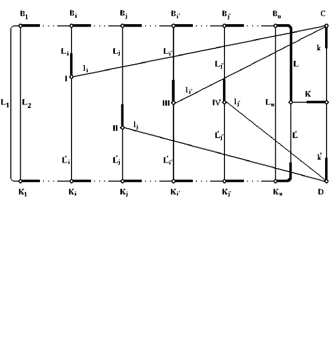
Figure 4: The recoupling matrix for the Fano angular calculation scheme.

Now let us treat a case when three distinct shells are acted upon by the operator. For example, the matrix element of operator $\widehat{G}(ij,ij^{\prime})$ is sought. Then in the recoupling matrix the node III will be on $L_{i}$ line (see Figure 4). This means that there will be two nodes on the resulting orbital moment $L_{i}$ line of shell $i$. These will be nodes I and III. The resulting orbital moment $L_{i}$ of the shell $i$ of bra function is attributed to the line connecting nodes $B_{i}$ and I. The resulting orbital moment $L^{\prime}_{i}$ of the shell $i$ of ket function is attributed to the line between nodes III and $K_{i}$. Finally, characteristics $L^{\prime\prime}_{i}$ of all possible intermediate momenta for that particular shell, which are summed over, are attributed to the line between nodes I and III. So, in treating the operator acting upon three distinct shells, an intermediate sum in the recoupling matrix appears. Similarly, two intermediate sums occur when two distinct shells are acted upon by the operator. And when it acts upon one shell only, three intermediate sums are present. The lines $k$, $k^{\prime}$ and $K$ in the recoupling matrix represent the structure of two- particle operator in $l$ - space. See Tutlys [66], Grant [8] for details.

This is also valid for the exchange term, only the line $l_{i^{\prime}}$ must be connected to the node D, and line $l_{j^{\prime}}$ - to the node C.

The first program to calculate the recoupling matrices of this type, NJSYM, was written by Burke [16]. It performs the calculations in two stages: 1) the recoupling matrix is expressed as a sum of products of the $6j$ - coefficients; 2) this expression is used in calculation.

Tutlys [66] wrote a program to calculate angular parts of matrix elements, ANGULA, which expressed the recoupling matrix in terms of Clebsch - Gordan coefficients before the actual calculations. While finding the recoupling matrix by the Clebsch - Gordan coefficient summation, this program eliminates trivial coefficients from the expression.

Bar-Shalom and Klapisch [17] developed a new program NJGRAF. This program calculates the recoupling matrix in several stages. On the basis of graphical methodology by Yutsis, Levinson and Vanagas [48], the recoupling matrix is analysed graphically and an optimal expression is found. Afterwards, the value of recoupling matrix itself is calculated. An analogous program RECOUP was written by Lima [67], and a program NEWGRAPH was written by Fack et al [68]. All these (NJGRAF, RECOUP and NEWGRAPH) are based on the same principle. An optimal analytical expression for the recoupling matrix is obtained by graphical method, and then the calculations are carried out according to it. But the optimal expressions they find are different quite often, and are not really optimal.

As it was mentioned above, the methodology of angular calculation based on the Fano calculation scheme has a shortcoming that the intermediate sums appear in complex recoupling matrices. Due to these summations and the complexity of the recoupling matrix itself, the associated computer codes become rather time consuming. A solution to this problem was found by Burke et al [9]. They tabulated separate standard parts of recoupling matrices along with coefficients of fractional parentage at the beginning of a calculation and then used them later to calculate the coefficients needed.

Computer codes by Glass [6], Glass and Hibbert [7], Burke et al [9], Fischer [69], Fischer [70] and Dyall et al [71] utilize the program NJSYM (Burke [16]) or NJGRAF (Bar-Shalom and Klapisch [17]) for the calculation of recoupling matrices. Both are rather time consuming when calculating matrix elements of complex operators or electronic configurations when calculating matrix elements of complex operators or electronic configurations with many open shells. In order to simplify the calculations, Cowan [2] suggested grouping matrix elements into ’classes’ (see Cowan [2], Figure 13-15). Unfortunately this approach was not generalized to all two-electron operators. Perhaps this is the reason why Cowan’s approach is not widely used although the program itself, based on this approach is widely used.

Gaigalas et al [33] proposed a methodology where the analytical expressions for recoupling matrices are obtained for the most general case. In this methodology, analogically as in Cowan [2], the matrix elements are attributed to four different groups. The operators acting upon only one shell belong to the first group (distribution 1 from Table 1), the ones acting upon two - to the second (distributions 2 - 10 from Table 1), upon three - to the third (distributions 11 - 18 from Table 1), and upon four - to the fourth group (distributions 19 - 42 from Table 1) respectively. Each group has a different recoupling matrix, $R_{1}$ - $R_{2}$. They all are shown in Figures 5 - 8.

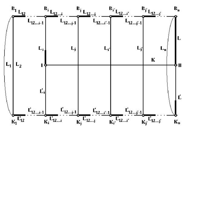
Figure 5: Diagram $R_{1}$ representing the recoupling matrix $R\left(\lambda_{i},\lambda_{j},\lambda_{i}^{\prime},\lambda_{j}^{\prime},\Lambda^{bra},\Lambda^{ket},\Gamma\right)$ when a two-particle operator acts upon a single shell.

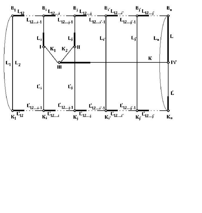
Figure 6: Diagram $R_{2}$ representing the recoupling matrix $R\left(\lambda_{i},\lambda_{j},\lambda_{i}^{\prime},\lambda_{j}^{\prime},\Lambda^{bra},\Lambda^{ket},\Gamma\right)$ when a two-particle operator acts upon a two shell.

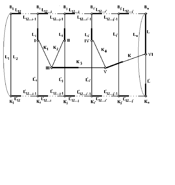
Figure 7: Diagram $R_{3}$ representing the recoupling matrix $R\left(\lambda_{i},\lambda_{j},\lambda_{i}^{\prime},\lambda_{j}^{\prime},\Lambda^{bra},\Lambda^{ket},\Gamma\right)$ when a two-particle operator acts upon a three shell.

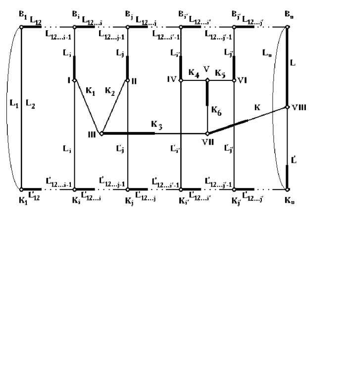
Figure 8: Diagram $R_{4}$ representing the recoupling matrix $R\left(\lambda_{i},\lambda_{j},\lambda_{i}^{\prime},\lambda_{j}^{\prime},\Lambda^{bra},\Lambda^{ket},\Gamma\right)$ when a two-particle operator acts upon a four shells.

6.1 One interacting shell

Let us treat the recoupling matrix $R_{1}$ first (see Figure 5). It represents the case when a physical two-particle operator acts upon a single shell. Here, similarly as in Figure 4, the graphical technique of Jucys and Bandzaitis [49] is used. The bra and ket functions are represented as in Figure 4. As the two-particle operator acts upon only one shell in this case, this operator may be treated as a single - particle one from the recoupling matrix point of view. Using a graphical rule allowing one to cut two lines and connect the loose ends, we disconnect the nodes $B_{1}$ and $K_{1}$ from the general recoupling matrix. The part separated from recoupling corresponds to delta - functions only, $\delta(L_{12},L^{\prime}_{12})$, $\delta(L_{1},L_{2},L_{12})$. In addition, using graphical technique it is possible to cut all the nodes until $B_{i}$ and $K^{\prime}_{i}$ out of the general recoupling matrix. All the cut nodes contribute the same delta functions which may be written as $\delta(L_{12..i-1},L^{\prime}_{12..i-1})$, $\delta(L_{12..i-1},L_{i},L_{12..i+1})$.

In the next stage, it remains to treat the part of recoupling matrix from the nodes $B_{i}$ and $F_{i}$ up to $B_{u}$ and $K_{u}$. Beside that, the lines $L_{12..i-1}$ and $L^{\prime}_{12..i-1}$ are connected in this remaining diagram. Before obtaining the analytical expression for the remaining recoupling matrix we introduce a notation $A_{1}(+-+-;J_{1}J_{2}J_{12};J_{3}JJ_{32})$. It will help us to describe the procedure of obtaining analytical expression for the remaining recoupling matrix in a simpler way. So, the diagram in Figure 9 is denoted as $A_{1}(+-+-;J_{1}J_{2}J_{12};J_{3}JJ_{32})$. It equals to

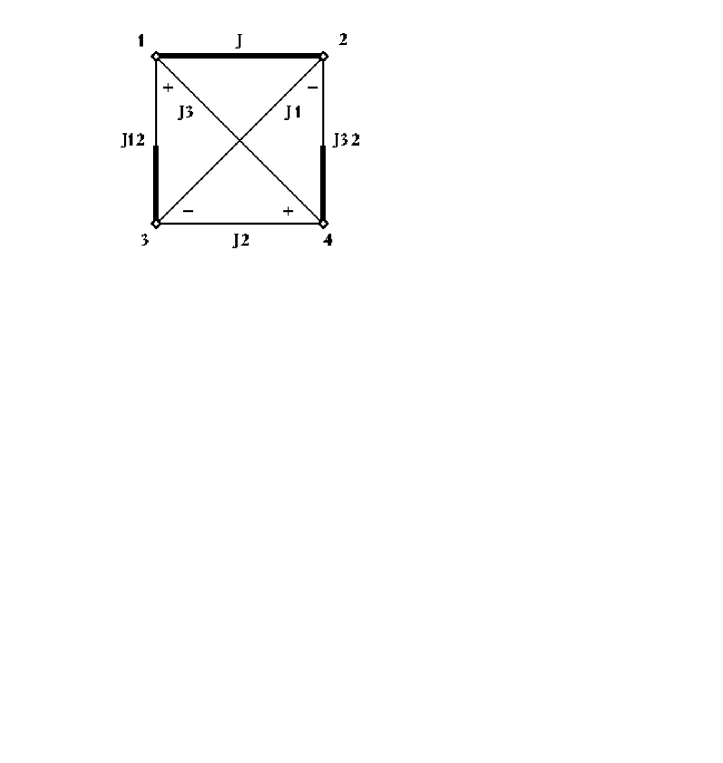
Figure 9: Diagram corresponding to the notation $A_{1}(+-+-;J_{1}J_{2}J_{12};J_{3}JJ_{32})$.

$$A_{1}(+-+-;J_{1}J_{2}J_{12};J_{3}JJ_{32})=\left(-1\right)^{2j}\left[j_{12},j_{32}\right]^{1/2}\left\{\begin{array}[]{ccc}J_{1}&J_{2}&J_{12}\\ J_{3}&J&J_{32}\end{array}\right\}.$$ (72)

Now, using the graphical rule of cutting three lines, we cut out the nodes $I$, $B_{i}$ and $K_{i}$ from the recoupling matrix. Thus we obtain a diagram $A_{1}(--++;KL^{\prime}_{i}L_{i};L_{12..i-1}LL^{\prime}_{12..i})$. This coefficient in the paper by Gaigalas et al [33] is denoted as $C_{1}$, and equals to

$$C_{1}=\left(-1\right)^{\varphi}\left[L_{a},T^{\prime}\right]^{1/2}\left\{\begin{array}[]{ccc}k&L_{a}^{\prime}&L_{a}\\ J&T&T^{\prime}\end{array}\right\}.$$ (73)

The diagram is cut from the nodes $B_{j}$ and $K_{j}$ up to $B_{u}$ and $K_{u}$ in the same way. It is expressed in terms of diagrams

$$\begin{array}[b]{c}C_{2}\left(K,k_{\min},k_{\max}\right)=\displaystyle{\stackrel{{\scriptstyle k_{\max}}}{{\prod_{i=k_{\min}}}}}A_{1}(+-+-;KL^{\prime}_{12...i}L_{12...i};L_{i}L_{12...i-1}L^{\prime}_{12...i-1}).\end{array}$$ (74)

It is easy to notice that $C_{2}\left(K,k_{\min},k_{\max}\right)$ corresponds to the coefficient $C_{2}\left(K,k_{\min},k_{\max}\right)$ defined in Gaigalas et al [33].

6.2 Two interacting shells

Before going into investigation of the recoupling matrix pictured in Figure 6, we denote the diagram $A_{2}$ (see Figure 10 ) as

$A_{2}(-++---;J_{1}J_{2}J_{12};J_{3}J_{4}J_{34};J_{13}J_{24}J)$. Its analytical expression is

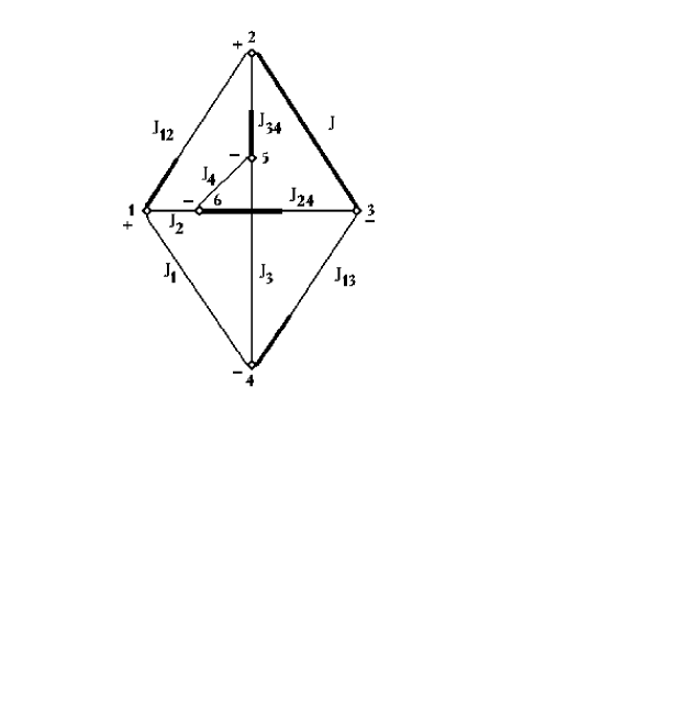
Figure 10: Diagram corresponding to the notation $A_{2}(-++---;J_{1}J_{2}J_{12};J_{3}J_{4}J_{34};J_{13}J_{24}J)$.

$$A_{2}(-++---;J_{1}J_{2}J_{12};J_{3}J_{4}J_{34};J_{13}J_{24}J)=\left[J_{12},J_{34},J_{13},J_{24}\right]^{1/2}\left\{\begin{array}[]{ccc}J_{1}&J_{2}&J_{12}\\ J_{3}&J_{4}&J_{34}\\ J_{13}&J_{24}&J\end{array}\right\}.$$ (75)

In the $A_{2}$ diagram, first the signs of nodes 1-6, and then the moments are presented.

While investigating the recoupling matrix (see Figure 6) it is easy to notice that there is an additional graphic element. After cutting this out, we get a diagram the further investigation of which is very similar to the investigation of $R_{1}$. That additional matrix element is

$A_{2}(-++---;L^{\prime}_{12..j-1}K_{1}L_{12..j-1};J^{\prime}_{j}K_{2}L_{j};L^{\prime}_{12..j}KL_{12..j})$. It is obtained by cutting the nodes $B_{j}$, $II$, $III$, $K_{j}$ out of the diagram $R_{2}$. After doing this, the diagram under investigation is split into two diagrams closely resembling the recoupling matrix $R_{1}$. As they are cut in the very same way as $R_{1}$ is, we will not stop at recoupling matrix $R_{2}$ for details.

6.3 Three interacting shells

In the methodology presented in Gaigalas et al [33], the recoupling matrix is represented by a diagram $R_{3}$ (see Figure 7) when the two-particle operator is acting upon three shells. Similarly as for the recoupling matrix $R_{2}$, the cutting out of nodes $B_{j}$, $II$, $III$ and $K_{j}$ leads to a diagram $A_{2}(-++---;L^{\prime}_{12..j-1}K_{1}L_{12..j-1};J^{\prime}_{j}K_{2}L_{j};L^{\prime}_{12..j}K_{3}L_{12..j})$, and the cutting out of nodes $B^{\prime}_{i}$, $IV$, $V$ ir $K^{\prime}_{i}$ leads to a diagram

$A_{2}(-++---;L^{\prime}_{12..i^{\prime}-1}K_{3}L_{12..i^{\prime}-1};J^{\prime}_{i^{\prime}}K_{4}L_{i^{\prime}};L^{\prime}_{12..i^{\prime}}KL_{12..i^{\prime}})$. In that case the diagram splits up into three simple diagrams, the further investigation of which is analogous to that of $R_{1}$ recoupling matrix.

6.4 Four interacting shells

The most complex recoupling matrix $R_{4}$ (see Figure 8) comes into view when all the second quantization operators act upon different shells. The part of this recoupling matrix from nodes $B_{1}$ and $K_{1}$ to nodes $B_{i^{\prime}}$ and $K_{i^{\prime}}$, and also from nodes $B_{j^{\prime}}$ and $K_{j^{\prime}}$ to nodes $B_{u}$ and $K_{u}$ is very similar to the recoupling matrices described above, therefore their investigation is the same as that of the diagrams described earlier. We will investigate in more detail the part of diagram from nodes $B_{i^{\prime}}$ and $K_{i^{\prime}}$ to nodes $B_{j^{\prime}}$ and $K_{j^{\prime}}$. That is pictured in Figure 11. After cutting the diagram across four lines $L_{12...i^{\prime}}$, $K_{4}$, $K_{3}$ and $L^{\prime}_{12...i^{\prime}}$ and connecting these according the graphical technique of Jucys and Bandzaitis [49] with a generalized Clebsch-Gordan coefficient, then connecting the lines $L_{12...i^{\prime}-1}$, $K_{3}$ and $L^{\prime}_{12...i^{\prime}-1}$ with an ordinary Clebsch-Gordan coefficient, we obtain a diagram which is expressed via two $6j$-coefficients. The exact analytical expression of this diagram is presented in the paper by Gaigalas et al [33] (see expresion (29)).

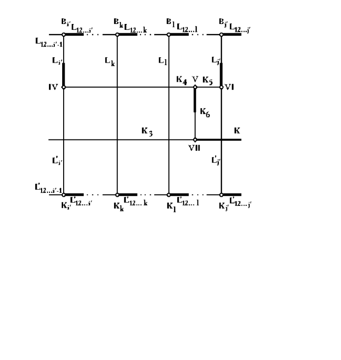
Figure 11: The most complex part of the recoupling matrix $R_{4}$.

After cutting the nodes $B_{j^{\prime}}$, $V$, $VI$, $VII$ and $K_{j^{\prime}}$ out of the remaining part and investigating the obtained diagram according to the Jucys and Bandzaitis [49] technique, we obtain a diagram which corresponds to a $12j$- coefficient. The analytical expression of that is presented in paper by Gaigalas et al [33], expr. (31).

If a shell $n_{j^{\prime}}l_{j^{\prime}}$ is beside shell $n_{i^{\prime}}l_{i^{\prime}}$, i.e. there are no additional nodes between nodes $B_{i^{\prime}}$, $K_{i^{\prime}}$ and $B_{j^{\prime}}$, $K_{j^{\prime}}$, then the additional graphical elements vanish. So, we obtained the full analytical expression of recoupling matrix $R_{4}$. If between the abovementioned shells a single additional shell is present, then we obtain an additional diagram which is expressed as a product of two $6j$-coefficients (see (30) from Gaigalas et al [33]). If the number of shells is greater, then the obatined diagram in the most general case is written via (32) from Gaigalas et al [33].

7 Conclusion

The methodology that is based on the second quantization in coupled tensorial form, on the angular momentum theory in three spaces (orbital, spin and quasispin), on the Wick’s theorem and on the generalized graphical technique of angular momentum, give the possibility to efficiently calculate the matrix elements of energy operators in general case (Gaigalas and Rudzikas [32], Gaigalas et al [33], this paper). The main ideas of this methodology are:

1. A number of theoretical methods is known in atomic physics that facilitate a lot the treatment of angular part of matrix elements. These are the theory of angular momentum, its graphical representation, the quasispin, the second quantization and its coupled tensorial form. But while treating the matrix elements of physical operators in general, the methods mentiond above are applied only some part, or very inefficiently.

   An idea is presented and carried out in the work Gaigalas and Rudzikas [32], Gaigalas et al [33] and this paper, of unifying all these methods in order to optimize the way to treat matrix elements of physical operators, to investigate efficiently even the most complex cases of atoms and ions.

2. The Wick’s theorem is widely known in the theory of atom. Up to now it was applied to the most general products of the operators of second quantization, i.e. when the particular arrays of quantum numbers for each operator of second quantization were not yet defined. In the methodology described there is proposed to apply the Wick’s theorem for the products of second quantization operators where they have the values of quantum numbers already defined. This allows one, using the methodology of second quantization in coupled tensorial form, to abtain immediately the optimal tensorial expressions for any operator. Then, in treting the matrix elements of physical operators, the advantages of a new modification of the Racah algebra are exploited to their full extent.

3. While analysing the physical operators presented as products of tensors $a^{(qsl)}$, $W^{(k_{q}k_{l}k_{s})}$, $[a^{(qsl)}\times W^{(k_{q}k_{l}k_{s})}]^{(K_{q}K_{l}K_{s})}$, $[W^{(k_{q}k_{l}k_{s})}\times a^{(qsl)}]^{(K_{q}K_{l}K_{s})}$,

   $[W^{(k_{q}k_{l}k_{s})}\times W^{(k^{\prime}_{q}k^{\prime}_{l}k^{\prime}_{s})}]^{(K_{q}K_{l}K_{s})}$, it is possible to obtain convenient analytical expressions for recoupling matrices that must be taken into account in finding the matrix elements (non-diagonal with respect to configuration included) of any physical operator between complex configurations (with any number of open shells).

4. An idea is proposed and carried out, concerning the most efficient way to apply the tensor algebra and the quasispin formalism in the most general case, for the diagonal and the non-diagonal matrix elements as well, when the bra- and ket- functions have any number of open shells.

The combination of all these improvements allows to efficiently account for correlation efects practically for any atom or ion of periodical table.

References

• [1] C.F. Fischer, The Hartree-Fock Method for Atoms (Wiley, New York, 1977).
• [2] R.D. Cowan, The Theory of Atomic Structure and Spectra (Berkeley, CA: University of California Press 1981).
• [3] A.P. Jucys and A.J. Savukynas, Mathematical Foundations of the Atomic Theory (Mintis, Vilnius, 1973) (in Russian).
• [4] A.A. Nikitin and Z. Rudzikas, Foundations of the Theory of the Spectra of Atomis and Ions (Nauka, Moscow, 1983) (in Russian).
• [5] Z. Rudzikas, Theoretical Atomic Spectroscopy (Cambridge Univ. Press, Cambridge, 1997).
• [6] R. Glass, ”Reduced matrix elements of tensor operators”, Comput. Phys. Commun., V. 16, p. 11-18 (1978).
• [7] R. Glass and A. Hibbert, ”Relativistic effects in many electron atoms”, Comput. Phys. Commun., V. 16, p. 19-34 (1978).
• [8] I.P. Grant, ”Relativistic atomic structure”, Math. Comput. Chem., V. 2, p. 1-71 (1988).
• [9] P.G. Burke, V.M. Burke and K.M. Dunseath, ”Electron-impact excitation of complex atoms and ions”, J. Phys. B: At. Mol. Opt. Phys., V. 27, p. 5341-5373 (1994).
• [10] U. Fano, ”Interaction between configurations with several open shells”, Phys. Rev. A., V. 140, No. 1A, p. A67-A75 (1965).
• [11] G. Racah, ”Theory of complex spectra I”, Phys. Rev., V. 61, p. 186-197 (1941).
• [12] G. Racah, ”Theory of complex spectra II”, Phys. Rev., V. 62, p. 438-462 (1942).
• [13] G. Racah, ”Theory of complex spectra III”, Phys. Rev., V. 63, p. 367-382 (1943).
• [14] G. Racah, ”Theory of complex spectra IV”, Phys. Rev., V. 76, p. 1352-1365 (1949).
• [15] A.P. Jucys and J.I. Vizbaraitė, ”On the method of calculation of matrix elements of the operators of atomic quantities in the case of complex configurations”, Proceedings of the Academy of Sciences of Lithuanian SSR, B Series V. 4 (27), p. 45-57 (1961) (in Russian).
• [16] P.G. Burke, ”A program to calculate a general recoupling coefficient”, Comput. Phys. Commun., V. 1, p. 241 (1970).
• [17] A. Bar-Shalom and M. Klapisch, ”NJGRAF - an efficient program for calculation of general recoupling coefficients by graphical analysis, compatible with NJSYM”, Comput. Phys. Commun., V. 50, p. 375-393 (1988).
• [18] A.P. Judd, Second Quantization and Atomic Spectroscopy (Baltimore, MD: John Hopkins Press, 1967).
• [19] A.P. Judd, in: Atomic, Molecular, and Optical Physics Handbook, edited by G. W. F. Drake (American Institute of Physics, Woodbury, NY, 1996).
• [20] Z. Rudzikas and J. Kaniauskas, Quasispin and Isospin in the Theory of Atom (Mokslas, Vilnius, 1984) (in Russian).
• [21] I. Lindgren and M. Morrison, Atomic Many-Body Theory (Springer Series in Chemical Physics 13) 2nd edn (Berlin, Springer, 1982).
• [22] G.V. Merkelis, G.A. Gaigalas and Z.B. Rudzikas, ”Irreducible tensorial form of the effective Hamiltonian of an atom and the diagrammatic representation in the first two orders of the stationary perturbation theory”, Liet. Fiz. Rink. (English translation– Sov. Phys. Coll.), V. 25, No. 6, p. 14-31 (1985).
• [23] P.H.M. Uylings, ”Energies of $N$ equivalent electrons expressed in terms of two-electron energies and independent three-electron parameters: a new complete set of orthogonal operators: I. Theory”, J. Phys. B: At. Mol. Phys., V. 17, p. 2375-2392 (1984).
• [24] P.H.M. Uylings, ”Applications of second quantization in the coupled form”, J. Phys. B: At. Mol. Phys., V. 25, p. 4391-4407 (1992).
• [25] F.R. Innes, ” Quasi-Spin Methods and Pairs of One-Particle CFP in the seniority scheme”, J. Math. Phys., V. 8, No. 4, p. 816-820 (1967).
• [26] V.V. Špakauskas, J.M. Kaniauskas and Z.B. Rudzikas, ”Tensorial properties of operators in quasi-spin space and their applications to the theory of many-electron atoms”, Liet. Fiz. Rink., V. 17, No. 5, p. 563-574 (1977).
• [27] V.V. Špakauskas, J.M. Kaniauskas and Z.B. Rudzikas, ”Reduced in quasi-spin space coefficients of fractional parentage and matrix elements of tensorial operators”, Liet. Fiz. Rink., V. 18, No. 3, p. 315 293 (1978). (English translation– Sov. Phys. Coll. 18(3), 1 (1978) from Allerton Press, New York).
• [28] U. Fano and A.R.P. Rau, Symmetries in Quantum Physics (Academic Press, New Yourk, 1996).
• [29] G.A. Gaigalas, Z.B. Rudzikas and C. Froese Fischer, ”Reduced coefficients (subcoefficients) of fractional parentage for $p$-, $d$-, and $f$-shells”, Atomic Data and Nuclear Data Tables, V. 70, p. 1-39 (1998).
• [30] G. Merkelis and G. Gaigalas, ”Expressions for reduced matrix elements of non-relativistic effective hamiltonian of atom in the first orders of stationary perturbation theory for configurations with two unifilled shells $n_{1}l_{1}^{N_{1}}~{}n_{2}l_{2}^{N_{2}}$”, in: Spectroscopy of Autoionized States of Atoms and Ions (Moscow, Scientific Council of Spectroscopy, 1985), p. 20-42.
• [31] G. Merkelis, ”Diagrammatic representation of perturbation expansion for open-shell atoms in coupled form”, Lithuanian Journal of Physics, V. 38, No. 3, p. 251-273 (1998).
• [32] G. Gaigalas and Z. Rudzikas, ”On the secondly quantized theory of the many-electron atom”, J. Phys. B: At. Mol. Opt. Phys., V. 29, p. 3303-3318 (1996).
• [33] G.A. Gaigalas, Z.B. Rudzikas and C. Froese Fischer, ”An efficient approach for spin-angular integrations in atomic structure calculations”, J. Phys. B: At. Mol. Opt. Phys., V. 30, p. 3747-3771 (1997).
• [34] G.A. Gaigalas, A. Bernotas, Z.B. Rudzikas and C. Froese Fischer, ”Spin-other-orbit operator in the tensorial form of second quantization”, Physica Scripta, V. 57, p. 207-212 (1998).
• [35] G. Gaigalas and Z. Rudzikas, ”Secondly quantized multi-configurational approach for atomic databases”, NIST Special Publication 926, p. 128-131 (1998).
• [36] Z. Rudzikas, ”New version of Racah algebra in atomic spectroscopy”, Comment. At. Mol. Phys., V. 26, No. 5, p. 269-286 (1991).
• [37] G.V. Merkelis, J. Kaniauskas and Z.B. Rudzikas, ”Formal methods of the stationary perturbation theory for atoms”, Liet. Fiz. Rink. (English translatin– Sov. Phys. Coll), V. 25, No. 5, p. 21-30 (1985).
• [38] W. Eissner, M. Jones and H. Nussbaumer, ”Techniques for the calculation of atomic structure and radiative data including relativistic corrections”, Comput. Phys. Commun., V. 8, p. 270-306 (1974).
• [39] N.R.J. Badnell, ”On the effects of the two-body non-fine-structure operators of the Breit-Pauli Hamiltonian”, Phys. B: At. Mol. Phys., V. 30, p. 1-11 (1997).
• [40] A. de Shalit and I. Talmi, Nuclear Shell Theory (New York, Academic Press, 1963).
• [41] S. Feneuille, ”Hamiltonien de contact spin-spin et interaction Coulombienne”, Phys. Lett. V. 28A, No. 2, p. 92-93 (1968).
• [42] G.C. Wick, ”The evaluation of the collision matrix”, Phys. Rev., V. 80, No. 2, p. 268-272 (1950).
• [43] N.N. Bogoliubov, D.V. Shirkov, Introduction to the Theory of Quantized Fields (Wiley, New Yourk, 1959).
• [44] A.L. Fetter, J.D. Walečka, Quantum Theory of Many-Particle Systems (McGraw-Hill, New York, 1971).
• [45] G. Gaigalas, J. Kaniauskas, Z. Rudzikas, ”Diagramatic technique of the angular momentum theory and of the second quantization”, Liet. Fiz. Rink. (English translation– Sov. Phys. Coll), V. 25, No. 6, p. 3-13 (1985).
• [46] G. Gaigalas, ”Diagramatic approach to irreducible tensorial operators and its application to perturbation theory”, in: Spectroscopy of Autoionized States of Atoms and Ions (Moscow, Scientific Council of Spectroscopy, 1985), p. 43-61.
• [47] G.V. Merkelis, G.A. Gaigalas, J. Kaniauskas and Z.B. Rudzikas, ”Application of the graphical methods of angular momentum theory to the investigation of the expansion of stationary perturbation theory”, Izv. Vyssh. Uchebn. Zaved. Fiz.,V. 50, No. 7, p. 1403-1410 (1986).
• [48] A.P. Yutsis, I.B. Levinson and V.V. Vanagas, The Theory of Angular Momentum (Israel Program for Scientific Translation, Jerusalem 1962).
• [49] A.P. Jucys and A.A. Bandzaitis, Theory of Angular Momentum in Quantum Mechanics (Mokslas, Vilnius, 1977), (in Russian).
• [50] D.M. Brink and G.R. Satcher, Angular Momentum (Oxford, Clarendon Press, 1968).
• [51] E. El-Baz, Traitement Graphique de l’algebra des Moments Angulaires (Paris, Masson, 1969).
• [52] G. Gaigalas, G. Merkelis, ”Application of the method of irreducible tensorial operators to study the expansion of stationary perturbation theory”, Acta Phys. Hungarica, V. 61, p. 111-114 (1987).
• [53] J.M. Kaniauskas and Z.B. Rudzikas, ”On expressing of the ransformation matrices in terms of $3nj$-coefficients and some $21j$-coefficients”, Liet. Fiz. Rink., V. 13, No. 2, p. 191-205 (1973).
• [54] A.P. Jucys, Z.B. Rudzikas and A.A. Bandzaitis, ”The graphical representation of the matrix elements of irreducible tensor operators”, Liet. Fiz. Rink., V. 5, No. 1, p. 5-12 (1965).
• [55] K.-N. Huang and A.F. Starace, ”Graphical approach to the spin-orbit interation”, Phys. Rev. A, V. 18, No. 2, p. 354-379 (1978).
• [56] A. Bolotin, Y. Levinson and V. Tolmachev, ”Angular integration of feynman diagrams in field perturbation theory of atoms”, Liet. Fiz. Rink., V. 4, No. 1, p. 25-33 (1964).
• [57] B.R. Judd, Operator Techniques in Atomic Spectroscopy (Princeton, New Jersey, Princeton University Press 1998).
• [58] C.W. Nielson and G. Koster, Specroscopic Coefficients for the $p^{n}$, $d^{n}$, and $f^{n}$ Configurations (MIT Press, Cambridge, MA, 1963).
• [59] R.I. Karazija, Ya. I. Vizbaraitė, Z.B. Rudzikas and A.P. Jucys, Tables for the Calculation of Matrix Elements of Atomic Quantities, (Moscow, 1967); English translation by E.K. Wilip, ANL-Trans-563 (National Technical Information Service, Springfield, Va., 1968).
• [60] H. Horie, ”Spin-spin and Spin-other-orbit Interactions”, Progress of Theoretical Physics, V. 10, No. 3, p. 296-308 (1953).
• [61] R.I. Karazija, J. Vizbaraitė and A. Jucys, ”On the calculation of the matrix elements of the ”spin-orbit” interaction energy operator for many-electron atoms”, Liet. Fiz. Rink., V. 6, no. 4, p. 487-496 (1966).
• [62] J. Vizbaraitė, R.I. Karazija, J. Grudzinskas and A. Jucys, ”The matrix elements of the ”spin-orbit” interaction energy operator for an open shell of atomic electrons, being outside close shells”, Liet. Fiz. Rink., V. 7, No. 1, p. 5-26 (1967).
• [63] R.I. Karazija, J. Vizbaraitė and A. Jucys, ”On the calculation of the matrix elements of the ”spin-spin” interaction energy operator for many-electron atoms”, Liet. Fiz. Rink., V. 6, No. 4, p. 479-486 (1966).
• [64] B.G. Wybourne, Spectroscopic Properties of Rare Earths (New York, John Wiley & Sons, Inc.: 1965).
• [65] R. Karazija, Introduction to the Theory of X-Ray and Electronic Spectra of Free Atoms, (Mokslas, Vilnius, 1997). English translation by Plenum Publishing Corporation, New York, 1996).
• [66] V.I. Tutlys, ”A program to calculate the matrix elements in multi-configuration approximation”, in: Sbornik Programm Po Matematicheskomy Obespecheniju Atomnyh Raschotov. Vipusk 4. (Vilnius, 1980) (in Russian).
• [67] P.M. Lima, ”A program for deriving recoupling coefficients formulae”, Comput. Phys. Commun., V. 66, p. 89 (1991).
• [68] V. Fack, S.N. Pitre and J. Van der Jeugt, ”Calculation of general recoupling coefficients using graphical methods”, Comput. Phys. Commun., V. 101, p. 155-170 (1997).
• [69] C.F. Fischer, ”A general multi-configuration Hartree-Fock program”, Comput. Phys. Commun., V. 14, p. 145 (1978).
• [70] C.F. Fischer, ”The MCHF atomic-structure package”, Comput. Phys. Commun., V. 64, No. 3, p. 369-398 (1991).
• [71] K.G. Dyall, I.P. Grant, C.T. Johnson, F.A. Parpia and E.P. Plummer, ”GRASP: a general-purpose relativistic atomic structure program”, Comput. Phys. Commun. V. 55, p. 425-455 (1989).