Projecting to a Slow Manifold:
Singularly Perturbed Systems and Legacy Codes.

Abstract

The long-term dynamics of many dynamical systems evolve on an attracting, invariant “slow manifold” that can be parameterized by a few observable variables. Yet a simulation using the full model of the problem requires initial values for all variables. Given a set of values for the observables parameterizing the slow manifold, one needs a procedure for finding the additional values such that the state is close to the slow manifold to some desired accuracy. We consider problems whose solution has a singular perturbation expansion, although we do not know what it is nor have any way to compute it. We show in this paper that, under some conditions, computing the values of the remaining variables so that their $(m+1)$st time derivatives are zero provides an estimate of the unknown variables that is an $m$th-order approximation to a point on the slow manifold in sense to be defined. We then show how this criterion can be applied approximately when the system is defined by a legacy code rather than directly through closed form equations.

Keywords: Initialization, DAEs, Singular Perturbations, Legacy Codes, Inertial Manifolds

1 Introduction

The derivation of reduced dynamic models for many chemical and physical processes hinges on the existence of a low-dimensional, attracting, invariant “slow manifold” characterizing the long-term process dynamics. This manifold is parameterized by a small number of system variables (or “observables”, functions of the system variables): when the dynamics have approached this manifold, knowing these observables suffices to approximate the full system state. A reduced dynamic model for the evolution of the observables can then in principle be deduced; the resulting simplification in complexity and in size can be vital in understanding and modeling the full system behavior. This reduction has been the subject of intense study from the theoretical, practical and computational points of view. Low-dimensional center-unstable manifolds are crucial in the study of normal forms and bifurcations in dynamical systems (e.g. [13]); the theory of Inertial Manifolds and Approximate Inertial Manifolds [6, 31] has guided model reduction in dissipative Partial Differential Equations; the study of fast/slow dynamics in systems of Ordinary Differential Equations is the subject of geometric singular perturbation theory (e.g. [7]). On the modeling side, the Bodenstein “quasi-steady state” approximation has long been the basis for the reduction of complex chemical mechanisms, described by large sets of ODEs ([2], see also the discussion by Turanyi [33]). More recently, an array of computational approaches have been proposed that bridge singular perturbation theory with large scale scientific computation for such problems; they include the Computational Singular Perturbation (CSP) approach of Lam and Goussis [23, 21, 22], and the Intrinsic Low-Dimensional Manifold approach of Maas and Pope [24]. The mathematical underpinnings of these methods have also been studied ([15, 34]). Lower-dimensional manifolds arise naturally also in the context of differential-algebraic equations, where the initialization problem has attracted considerable attention (e.g. [3]).

Remarkably, the same concept of separation of time scales and low-dimensional long-term dynamics underpins the derivation of “effectively simple” descriptions of complex systems. In this context, the detailed model is a collection of agents (molecules, cells, individuals) interacting with each other and their environment; the entire distribution of these agents that evolves through atomistic or stochastic dynamic rules. In many problems of practical interest it is possible to write macroscopic equations for the large-scale, coarse-grained dynamics of the evolving distribution in terms of only a few quantities, typically lower moments of the evolving distribution. In the case of isothermal Newtonian flow, for example, we can write closed evolution equations for the density and the momentum fields, the zeroth and first moments of the particle distribution over velocities. This is again a singularly perturbed problem; only in this case the higher moments of the evolving distribution have become quickly slaved to the lower ones (in this case stresses, after a few collisions, have become functionals of velocity gradients). Newton’s law of viscosity therefore represents a similar type of “slow manifold” as in the ODE case discussed above - fast variables (stresses) become functionals of velocity gradients, and the slow manifold is embodied in the closure: Newton’s law of viscosity. The use of slow manifolds in non-equilibrium thermodynamics, and more generally in the study of complex systems, is also a subject of intense current research (see the work of Gorban, Karlin, Oettinger and coworkers [12, 11], as well as [18, 19]) for some recent computational studies. In this context, one has an “inner simulator” at the microscopic or stochastic level for evolving the detailed distributions; a separation of time scales does not arise at this level, but rather at the level of the evolution of the statistics or moments of these distributions. Typically the lower moments of the evolving distributions parameterize the slow manifold, while the higher moments quickly evolve to functionals of the lower ones. Since we do not have explicit formulas for the equations at the coarse-grained, macroscopic level, the following interesting question arises: can we benefit from singular perturbation, when no closed form evolution equations are available, and the only tool at our disposal is a “black box” dynamic simulator of the detailed problem ? This is the problem we will address in this paper.

We will assume that we are given an evolutionary system which can be described by

$$u^{\prime} = p(u,v)$$ (1)

$$v^{\prime} = q(u,v)$$ (2)

where prime designates differentiation w.r.t. $t$, the dimensions of $u$ and $v$ are $N_{u}$ and $N_{v}$ respectively, and values, $u(0)$, are specified only for $u$. In the case of a legacy dynamic code, we may not even be given the formulas for these equations explicitly; instead, we may be given a time-stepper of the above system as a black-box subroutine: a code that, provided an initial condition for $u$ and $v$, will return an accurate approximation of $u$ and $v$ after a time interval (a reporting horizon) $\Delta T$. We wish to find $v(0)$ so that the solution is “close to a slow manifold.” This statement is deliberately vague because in practice we are proceeding on the belief that there exists a slow, attracting, invariant manifold that can be parameterized by $u$ and that the variables $v$, in some sense, “contain” the fast variables so that their values on the slow manifold can be computed from the values of $u$ at any time. (Note that we do not need to know which are the slow variables, only to be able to identify a set of variables sufficient to parameterize the slow manifold.) This implies that the manifold is the graph of a function $v=v(u)$ over the observables $u$. As we proceed, we will make these statements more precise. However, we will not cast them into the form of theorems because, even though this is possible, the conditions for the application of the theorems would be essentially impossible to verify in all but trivial problems. As with many numerical methods, the primary test of applicability is in the actual application.

We assume that the system can be expressed in terms of other variables, $x$ and $y$, of the same dimension as $u$ and $v$ respectively, and that in terms of $x$ and $y$ the system can be written in the usual singular perturbation form:

$$x^{\prime} = f(x,y)$$ (3)

$$\epsilon y^{\prime} = g(x,y)$$ (4)

where $x$ and $y$ are also of dimension $N_{u}$ and $N_{v}$, respectively. We will assume that their initial values are specified as $x(0)$ and $y(0)$, independent of $\epsilon$. The singular perturbation parameter, $\epsilon$, is associated with the gap, or ratio, between the “active” (slow) eigenvalues and the rightmost of the negative, inactive eigenvalues of the linearized problem, locally. We stress that we do not assume that we know how to express the equations in the form of eqs (3) and (4) nor do we have any knowledge of the transformation

$$u = u(x,y),\hskip 7.22743ptx(0,\epsilon)=x(0)$$ (5)

$$v = v(x,y),\hskip 7.22743pty(0,\epsilon)=y(0)$$ (6)

other than that we assume that it is well-conditioned and does not have large derivatives. We will consider singular perturbation expansions in $\epsilon$, even though the parameter is not identified (and cannot be varied). The functions $f$ and $g$ could also involve the parameter $\epsilon$, but that serves little in this presentation other than to complicate the algebra.

The standard singular perturbation expansion for the solution of eqs (3) and (4) takes the form:

$$x(t,\epsilon) = \sum_{n=0}^{\infty}\epsilon^{n}X_{n}(t)+\epsilon\sum_{n=0}^{\infty}\epsilon^{n}\xi_{n}(\tau)$$ (7)

$$y(t,\epsilon) = \sum_{n=0}^{\infty}\epsilon^{n}Y_{n}(t)+\sum_{n=0}^{\infty}\epsilon^{n}\eta_{n}(\tau)$$ (8)

This involves an outer solution $(X(t),Y(t))$, that is smooth in the sense that its time derivatives are modest, and an inner solution, $(\xi(\tau),\eta(\tau))$, that captures the fast boundary layer where the solution typically changes like $e^{-t/\epsilon}=e^{-\tau}$. Both outer and inner solutions are expressed as power series in $\epsilon$, the latter as a function of the stretched time $\tau$. The inner solution is fast in the sense that each differentiation by $t$ introduces a multiplier of $1/\epsilon$.

We define the slow manifold as the manifold that contains all solutions of eqs (3) and (4) of the form eqs (7) and (8) with the inner solution identically zero. This is an invariant manifold. We say that a solution is an $m$th-order approximation to a slow manifold solution if it has the form in eqs (7) and (8) with the first $m+1$ terms of the inner solution expansion identically zero. A point $(u,v)$ is an $m$-th order approximation to the slow manifold, or $m$-th order close to the slow manifold, if it lies on an $m$-th order approximate solution.

We want to stress that we are not proposing a technique for finding the singular perturbation expansion. Rather, we are using the ideas as a scaffold for the theoretical justification of the proposed computational method. It is possible that the method will provide answers even when the singular perturbation expansions do not converge (although in that case we have no justification other than an intuitive one). The procedure we propose for finding the $v$ values that are close to the slow manifold given the $u$ values is to find values of $v$ that approximately solves the $N_{v}$ dimensional non-linear equation

$$\frac{d^{m+1}v}{dt^{m+1}}=0$$ (9)

which we call “the [$(m+1)$-st] derivative condition.” (Compare this with the “bounded derivative principle” [20] which requires the first $m$ time derivatives to be of order 1. That condition can be applied to problems with fast oscillating solutions. Ours can not, but it is simpler to apply to the types of problems we consider.)

Note that eq. (9) is a local condition - that is, it is applied at a single time - which we will take to be $t=t_{0}=0$ - to determine a value of $v$ corresponding to a given value of $u$. A solution of eqs (1) and (2) starting from these values of $u$ and $v$ will not satisfy eq. (9) for $t>0$ - but we do expect the solution to be close to the slow manifold. Intuitively the condition in eq. (9) finds a point close to the slow manifold because differentiation “amplifies” rapidly varying components more than slowly varying components, so eq. (9) seeks a region where the fast components are small. We will suggest ways in which eq. (9) can be solved approximately in practical codes, even those based on a legacy code for the integration of eqs (1) and (2).

While the approach will be presented and implemented for singularly perturbed sets of ODEs, the “legacy code” formulation is appropriate also in cases where the inner simulator is not a differential equation solver, but rather a microscopic / stochastic simulator. In the equation free approach we have been developing for the computer-assisted study of certain classes of complex systems, the variables $u$ correspond to macroscopic observables of a microscopic simulation (typically, moments of a stochastically or deterministically evolving distribution). In this case $v$ corresponds to statistics of the evolving distribution (e.g. higher moments) that become quickly slaved to (become functionals of) the observables $u$; thus the analogy of a slow manifold persists in moments space for the evolving distribution.

The paper is organized as follows: In the next Section we will outline the theoretical basis for the derivative condition. In Section 3 we discuss ways in which the derivative condition can be approximately applied as a difference condition and used with legacy codes. Section 4 presents some simple examples of its application. We conclude with a brief summary and outline of the scope of the method and some of the challenges we expect to arise in its wider application.

2 Theoretical Basis

In this section we will show that the application of the condition in eq. (9) will lead to a $m$th-order approximation to the slow manifold under suitable smoothness and smallness conditions. We will start by sketching the parts of singular perturbation expansion theory that we need by paraphrasing the presentation in O’Malley’s monograph[26], particularly pp 46-52. We will use the same notation to make it easier for the reader who wishes to get more detail from that book.

In the following we will write $X_{n},~{}Y_{n},~{}\xi_{n}$, and $\eta_{n}$ to mean $X_{n}(t),~{}Y_{n}(t),~{}\xi_{n}(\tau)$, and $\eta_{n}(\tau)$. We recall from [26] that the $t$ and $\tau$ dependencies are treated separately, and that the terms in the outer expansion, $\{X_{n},Y_{n}\}$, are obtained term by term by substituting eqs (7) and (8) into eqs (3) and (4), and equating each outer term in $\epsilon^{n}$ to zero, starting with $n=0$. For $n=0$ we obtain the DAE:

$$X^{\prime}_{0} = f(X_{0},Y_{0}),\hskip 7.22743ptX_{0}(0)=x(0)$$ (10)

$$0 = g(X_{0},Y_{0})$$ (11)

The existence of a smooth solution of this equation for any $x(0)$ requires the assumption that $g_{y}$ is non-singular. (The existence of asymptotic expansions for the inner and outer components requires the stronger assumption that $g_{y}$ is a stable matrix.) Then, $Y_{0}$ is specified uniquely in terms of $X_{0}$ by eq. (11), say as

$$Y_{0}=\phi(X_{0}).$$

The $n$th term in the power series yields the DAE

$$X^{\prime}_{n} = f_{x}(X_{0},Y_{0})X_{n}+f_{y}(X_{0},Y_{0})Y_{n}+\tilde{f}_{n}$$ (12)

$$0 = g_{x}(X_{0},Y_{0})X_{n}+g_{y}(X_{0},Y_{0})Y_{n}+\tilde{g}_{n}$$ (13)

where the $\tilde{f}_{n}$ and $\tilde{g}_{n}$ are defined in terms of earlier terms in the outer expansion, $\{X_{j},Y_{j}\},j=0,\cdots,n-1$. The initial condition, $X_{j}(0)$, has to be specified. Since we have set $X(0)=x(0)$, $X_{j}(0)$ is obtained from eq. (7) by requiring that the $\epsilon^{j}$ term vanishes at $t=0$, which gives

$$X_{j}(0)=-\xi_{j-1}(0).$$ (14)

We are most interested in the way in which the inner terms are defined, since we wish to annihilate the first $m+1$ of these to get an $m$th-order approximation. These are obtained by considering the change in the inner terms as $\tau$ varies for arbitrarily small $\epsilon$, in other words, with $t=0$ and the outer solutions fixed at their initial values. Following [26] we consider terms in successive powers of $\epsilon$ and find that the $\epsilon^{0}$ terms satisfy:

$$\dot{\xi}_{0} = f(x(0),Y_{0}(0)+\eta_{0})-f(x(0),Y_{0}(0))$$ (15)

$$\dot{\eta}_{0} = g(x(0),Y_{0}(0)+\eta_{0})-g(x(0),Y_{0}(0))$$ (16)

where a dot represents differentiation w.r.t. $\tau=t/\epsilon$. If we have an initial value for $\eta_{0}(0)$ we can solve eq. (16) for $\eta_{0}$. Eq. (15) gives $\xi_{0}$ as an indefinite integral so it is determined by specifying $\xi_{0}$ at any point. This is normally done at $\tau=\infty$, in other words, at the end of the boundary layer. However, in our development here we will be showing that $\eta_{j}$ and $\xi_{j}$ are identically zero for $j\leq m$, so we will actually choose $\xi_{j}(0)=0$ (so that we also have $X_{j+1}(0)=0$ from eq. (14)). Subsequent inner terms satisfy

$$\dot{\xi}_{n} = f_{y}(x(0),Y_{0}(0)+\eta_{0})\eta_{n}+\hat{f}_{n}$$ (17)

$$\dot{\eta}_{n} = g_{y}(x(0),Y_{0}(0)+\eta_{0})\eta_{n}+\hat{g}_{n}$$ (18)

where $\hat{f}_{n}$ and $\hat{g}_{n}$ are functions of the earlier terms, $\{\xi_{j},\eta_{j}\},j=0,\cdots,n-1$. In particular, if all of these terms are zero, then $\hat{f}_{n}$ and $\hat{g}_{n}$ are zero. Eq. (18) can be solved if an initial value is known for $\eta_{n}(0)$. Once again, eq. (17) gives $\xi_{n}$ as an indefinite integral.

In the following we are going to show, one by one, that $\eta_{j}(0)=0$ for $j=0,1,\cdots,m$, and that we can then choose $\xi_{j}(0)=0$. Note that once we have shown that $\eta_{0}(0)=0$ then eqs (15) and (16) indicate that $\eta_{0}(\tau)=0$ and that $\xi_{0}(\tau)$ is constant, which we can make zero by choosing $\xi_{0}(0)=0$. Then it follows that $\hat{f}_{1}$ and $\hat{g}_{1}$ are identically zero. Repeating this argument, we see that if $\eta_{j}(0)=0,\xi_{j}(0)=0,j=0,\cdots,m$ then $\xi_{j}(\tau)$ and $\eta_{j}(\tau)$ are identically zero for $j\leq m$. This provides a solution that is an $m$th-order approximation.

Now we return to the original problem phrased in terms of $u$ and $v$. If we knew the transformation to $x$ and $y$ we would do better to work in that space, but our assumption is that, although a transformation exists, it is unknown and we have to work with $u$ and $v$. We want to show that if the $(m+1)$st derivative of $v$ is zero, then the point is $m$th-order close to the slow manifold. All terms below are evaluated at $t=0$ or $\tau=0$ - the time at which we are attempting to solve eq. (9). We will simplify the notation and write $\eta_{j}$ for $\eta_{j}(0)$ and similarly for other terms in the following. We have from eq. (6)

$$\frac{d^{m+1}v}{dt^{m+1}}=v_{y}\frac{d^{m+1}y}{dt^{m+1}}+{\rm other~{}terms}$$ (19)

where the other terms involve either partial derivatives of $v$ w.r.t. $x$ and/or multiple derivatives of $v$ w.r.t. $y$ and products of derivatives of $y$.

Substituting from eq. (8) into eq. (19) and extracting the lowest order term in $\epsilon$ ($\epsilon^{-m-1}$) we find that at $t=0$

$$\frac{d^{m+1}v}{dt^{m+1}}=\epsilon^{-m-1}v_{y}\frac{d^{m+1}\eta_{0}}{d\tau^{m+1}}+{\rm other~{}terms}+{\rm O}(\epsilon^{-m})$$ (20)

where now the other terms include products of a higher-order partial derivative of $v$ w.r.t. $y$ with more than one $\tau$-derivative of $\eta_{0}$ such that the sum of the levels of differentiation is $m+1$, that is, terms like

$$v_{yy}\frac{d^{k}\eta_{0}}{d\tau^{k}}\frac{d^{m+1-k}\eta_{0}}{d\tau^{m+1-k}}$$

and terms with higher partial derivatives and more derivatives of $\eta_{0}$ in the product. Note that whenever $\eta_{0}$ appears, it is always differentiated w.r.t. $\tau$ at least once. Also note that we do not get any terms involving $\xi_{0}$ because of the additional $\epsilon$ appearing in front of the inner solution expansion for $x$ in eq. (7).

Now we use eq. (16) to find the higher-order derivatives of $\eta_{0}$ w.r.t. $\tau$. We get for $p>1$

$$\frac{d^{p}\eta_{0}}{d\tau^{p}}=g^{p-1}_{y}\dot{\eta}_{0}+{\rm other~{}terms}$$ (21)

where the other terms involve $\dot{\eta}^{j}_{0}$ with $j>1$. Substituting eq. (21) in eq. (20) we arrive at

$$\frac{d^{m+1}v}{dt^{m+1}}=\epsilon^{-m-1}\left[v_{y}g^{m}_{y}\dot{\eta}_{0}+\sum_{j=2}^{m+1}v_{z}g_{z}\dot{\eta}^{j}_{0}\right]+{\rm O(}\epsilon^{-m})$$ (22)

where the notation $v_{z}g_{z}$ stands for sums of products of various partial derivatives of $v$ and $g$. Equating the leading term of the right-hand side of eq. (22) to zero, we now have a polynomial equation for $\dot{\eta}_{0}$ as

$$v_{y}g^{m}_{y}\dot{\eta}_{0}+\sum_{j=2}^{m+1}v_{z}g_{z}\dot{\eta}^{j}_{0}=0$$ (23)

One solution of this is

$$\dot{\eta}_{0}=0$$

and it is an isolated root as long as $v_{y}g_{y}$ is non-singular. Since we have assumed that $g_{y}$ is a stable matrix for the existence of a singularly perturbed solution (and hence a slow manifold) and that $v$ in some sense spans the fast variables (meaning that $v_{y}$ is non singular), this is no problem. If all other partial derivatives involved in eq. (23) are “of order one” then other solutions are also of order one - i.e., well separated from the zero solution. We will delay discussion of how to avoid the “wrong” solutions for the moment, and assume that we find the zero solution. (If the problem is linear, these other terms are null, so there are no other solutions, and it is only in the case of high non-linearity when the partial derivatives are large that these other solutions can become small and cause problems.)

If $\dot{\eta}_{0}=0$ then eq. (16) tells us that $\eta_{0}=0$ because we have assumed that $g_{y}$ is a stable matrix (in the domain of interest). This immediately implies that $\xi_{0}=0$ (or is a constant that can be absorbed into the outer solution, thus making $\xi_{0}=0$).

As discussed following eq. (18), the vanishing of $\eta_{0}$ and $\xi_{0}$ means that the last terms of eqs (17) and (18) are zero for $n=1$, making them look similar to eqs (15) and (16). Therefore the above argument can now be applied to show that $\eta_{1}$ and $\xi_{1}$ are zero. This argument can be repeated for higher-order terms as long as the power of $\epsilon$ in eq. (22) remains negative, in other words, until we have shown that

$$\eta_{j}=\xi_{j}=0,\hskip 36.135ptj=0,\cdots,m$$

Note that when we have made the $(m+1)$st derivative zero, the lower order derivatives will not be zero, or even small. This is because a small movement away from the slow manifold can make large changes in the derivatives of the inner solution. However, the difference between successive $v$ values as we make $m$ successively larger is small - of order $\epsilon^{m+1}$ as we go from the $m$-th to the $m+1$-st derivative condition as the $v$ values are converging to the slow manifold. Hence one way to solve for zeros of high-order derivatives would be to start by finding the zeros of the first order derivative, then repeating for successively higher-order derivatives, each step requiring smaller and smaller changes to $v$, until we have found the zeros of the $(m+1)$st derivatives using whatever computational process is appropriate. (The computational process is addressed in the next section.) This procedure helps address the issue of finding the smallest of multiple roots of eq. (23) since, for $m=0$, there is only one root so that the iteration for $m=1$ and larger $m$ starts with a good approximation. If the zero root is well separated from the others, we will converge to it.

3 Practical Implementation

It is often not practical to work with higher-order derivatives of a differential equation, either because they are algebraically complicated or because the equations are defined by a “legacy code” - that is, as an implementation of a step-by-step integrator that effectively cannot be change or analyzed. (The same would be true if part of the derivative calculations involved table look-up functions that could be difficult to differentiate.) Therefore, we are interested in methods that do not require direct access to the mathematical functions constituting the differential equation. The same rationale applies when the “inner simulator” simulates the system at a different level (i.e. in the form of an evolving microscopic or stochastic distribution). In this case we only have a time-$T$ map for the macroscopic observables, that results from running the microscopic simulator and monitoring the evolution of the observables (e.g. particle densities) in time [32, 10].

The obvious alternative is to use a forward difference approximation to the derivative, noting that if

$$\Delta^{m+1}v(t)\equiv\Delta^{m}v(t+H)-\Delta^{m}v(t)$$ (24)

with $\Delta^{0}v(t)=v(t)$, then

$$\Delta^{m+1}v(t)=H^{m+1}\frac{d^{m+1}v}{dt^{m+1}}+{\rm O}(H^{m+2})$$

It turns out that there is a straightforward way to implement a functional iteration to find a zero of the $(m+1)$-st forward difference, even if we only have a “ black box” code that integrates eqs (1) and (2). Suppose we have operators, $\phi$ and $\theta$, that, given values of $u(t)$ and $v(t)$, yield approximations to $u(t+H)$ and $v(t+H)$, namely

$$u(t+H)\approx\phi(u(t),v(t))$$ (25)

$$v(t+H)\approx\theta(u(t),v(t))$$ (26)

Letting $t_{n}=t_{0}+nH$ and applying eqs (25) and (26) $m+1$ times starting from $t=t_{0}$ we can compute approximations

$$u_{j+1}=\phi(u_{j},v_{j})\approx u(t_{j+1})$$ (27)

$$v_{j+1}=\theta(u_{j},v_{j})\approx v(t_{j+1})$$ (28)

for $j=0,\cdots,m$. The functional iteration to find a $v_{0}$ for a given $u_{0}$ such that the $(m+1)$-st difference is zero consists of the following steps:

1. Start with a given $u_{0}$ and a guess of $v_{0}$.

2. Set the iteration number $p=1$.

3. Set the current iterate $v_{0}^{(1)}=v_{0}$

4. Apply eqs (27) and (28) $m+1$ times starting from $u_{0},v_{0}^{(p)}$ to generate $v_{1}^{(p)},v_{2}^{(p)},\cdots,v_{m+1}^{(p)}$.

5. Compute $\delta=(-1)^{m}\Delta^{m+1}v_{0}^{(p)}$

6. If $\delta$ is small, the iteration has converged.

7. If $\delta$ is not small,

   $$v_{0}^{(p+1)}=v_{0}^{(p)}+\delta$$ (29)

8. Increment $p$ and return to step 4.

If the black box integrator provides a good integration (that is, it does not introduce spurious oscillations due to near instability) and $H$ is small enough, this process will converge on a zero of the difference.

As an illustration we consider the case $m=0$ and assume that the integrator is simply forward Euler with a step size such that its product with the magnitude of the largest eigenvalue is less than one. We see that the process for $v$ consists of computing

$$\delta=v_{1}-v_{0}\approx H\frac{dv}{dt}(t_{0}).$$

If this is insufficiently small, we replace $v_{0}$ with $v_{0}+\delta=v_{1}$. This is just the stationary projection process used in [8] and is related to the “reverse time” projective integration method in [9]. In the case of $m=1$ we compute $\delta$ as

$$\delta=-v_{2}+2v_{1}-v_{0}$$

If this is insufficiently small, we add it to $v_{0}$ to get a new $v_{0}$ given by

$$v_{0}=2v_{1}-v_{2}$$

This is precisely the linear interpolant through $v_{1}$ and $v_{2}$ back to the starting point. It is illustrated in Figure 1. (This Figure may be a little confusing because it is drawn in the $u-v$ plane to emphasize that $u$ is being held constant from iteration to iteration. The backwards interpolant, however, is really taking place in the $t-v$ plane.)

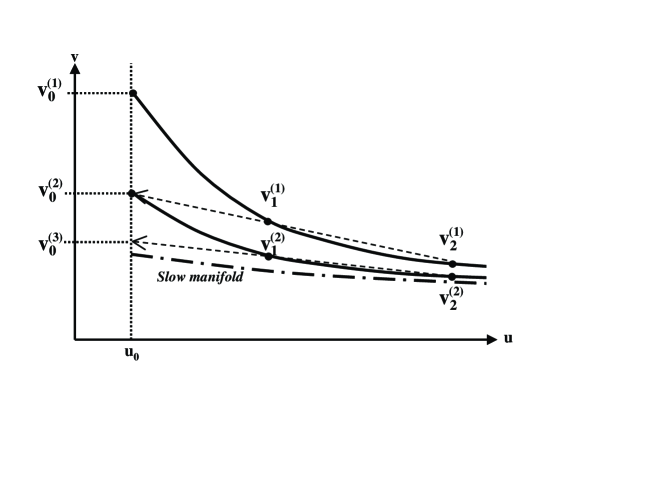
Figure 1: Iterative process for $m=1$.

The general iteration is equivalent to the obvious extension of that: an $m$th degree interpolant is passed through $v_{1},v_{2},\cdots,v_{m+1}$ to compute a new approximation to $v_{0}$. This is conveniently done using differences as described above.

Why does this iteration eq. (29) converge for small $H$ under reasonable circumstances? Intuitively, the forward integration exponentially damps the fast components more than they are amplified by the polynomial extrapolation backwards. In more mathematical terms, the iteration takes the form

$$v^{new}_{0}=v_{0}+\delta$$ (30)

If $\partial\delta/\partial v_{0}$ is negative definite and small, this will converge. We have

$$\partial\delta/\partial v_{0}=-(-H)^{m+1}\frac{\partial(\frac{d^{m+1}v}{dt^{m+1}})}{\partial v}+{\rm O}(H^{m+2})$$

The term

$$\frac{\partial(\frac{d^{m+1}v}{dt^{m+1}})}{\partial v}$$

is dominated by

$$\epsilon^{m+1}g_{y}^{m+1}$$

in powers of $\epsilon$. Since we have assumed that $g_{y}$ is a negative definite matrix for the existence of a singular perturbation expansion, convergence follows for small enough $H$.

In the above discussion we have used the attractivity of the manifold and, in effect, successive substitution in order to converge to a fixed point of our mapping. One can accelerate this computation by using fixed point algorithms, like Newton’s method; clearly, since no equations and Jacobians are available, the problem lends itself to matrix-free fixed point implementations like the Recursive Projection Method by Shroff and Keller [28] or Newton-Krylov implementations (see [16] and, for a GMRES-based implementation for timesteppers [17]).

4 Examples

We will consider three examples to illustrate the method. The Michaelis-Menten enzyme kinetics model is a classic example for singular perturbation (see [1] for a brief discussion on the history of the model and its analysis). Since it is a simple system we can make a direct comparison with an easily computable singular perturbation expansion. The second example is a realistic five-dimensional chemical reaction system with a one dimensional slow manifold. As in many real examples, we do not know the slow manifold, and can only show “plausibility” of our solution. The final example is a contrived five-dimensional non-linear system with a known two-dimensional slow manifold so that we can compute the “errors” as the distance from the slow manifold.

4.1 Michaelis-Menten equation

This is given in a singular perturbation form in [26] as

$$x^{\prime} = -x+(x+\kappa-\lambda)y$$ (31)

$$\epsilon y^{\prime} = x-(x+\kappa)y$$ (32)

with $x(0)=1$. For some simple tests we will take $\kappa=1$, $\lambda=0.5$, and $\epsilon=$ 0.1 and 0.01. (These are larger figures than typical for reactions, but we wish to show that the method works even for problems with a relative small gap, and also to have problems where the higher-order initializations are visibly different from the lowest order ones.)

The first few terms of the outer solution are

$$y=\frac{x}{x+\kappa}+\frac{\kappa\lambda x}{(x+\kappa)^{4}}\epsilon+\frac{\kappa\lambda x(2\kappa\lambda-3x\lambda-x\kappa-\kappa^{2})}{(x+\kappa)^{7}}\epsilon^{2}+{\rm O}(\epsilon^{3}).$$ (33)

In the following tests, we implemented the operators $\phi$ and $\theta$ in eqs (25) and (26) using $n$ steps of forward Euler with step size $h$. In all cases eq. (30) was iterated until $\delta$ was less than $10^{-14}$ (which is rather excessive, but we didn’t want any errors from premature termination to color the results). We ran with $m=0,\cdots,4$ and compared them with the first $m+1$ terms of eq. (33) through $m=2$. For $\epsilon=0.1$, the results are shown in Table 1 with $h=\epsilon/100$ and $n=1$, and in Table 2 with $h=\epsilon/10$ and $n=4$. The tables show the computed approximation to the slow manifold, $y(0)$, for $x(0)=1$. The tables also show the first $m$ terms of the asymptotic expansion for $m\leq 2$. As can be seen, the discrepancies are larger when $H=nh$ is larger.

A larger “integration time horizon” $H$ gives more rapid convergence. However, this means than the difference estimate is a less accurate approximation to the $(m+1)$-st derivative. Our theory shows that making the $(m+1)$-st derivative zero puts the solution on an $m$-th order approximation to the slow manifold. Any error in the derivative estimate creates an error of the same order in the solution, so we should choose the time horizon so that the errors in the derivative estimate are of the same order as those we are willing to tolerate in the approximation to the slow manifold. This suggests that an initial approximation could be calculated with a larger $H$ (and small $m$) to get faster convergence, and then $H$ could be reduced as $m$ is increased to increase the accuracy.

Table 1: Michaelis-Menten example with $\epsilon=0.1$, $h=\epsilon/100$ and $n=1$.

$m$	Computed $y$	Asymptotic $y$
0	0.500000000	0.500000000
1	0.503049486	0.503125000
2	0.503031986	0.503027344
3	0.503031924	-
4	0.503031924	-

Table 2: Michaelis-Menten example with $\epsilon=0.1$, $h=\epsilon/10$ and $n=4$.

$m$	Computed $y$	Asymptotic $y$
0	0.498886090	0.500000000
1	0.503067929	0.503125000
2	0.503035446	0.503027344
3	0.503035098	-
4	0.503035128	-

The next case, shown in Table 3, uses an $\epsilon$ smaller by a factor of 10. Because the higher-order terms in $\epsilon$ are now smaller, the agreement with the terms in the asymptotic expansion is better. (However, we are really interested in the agreement of the computed $v_{0}$ with the $v$ on the slow manifold, rather than with the ability to match the first few terms in the asymptotic expansion.)

Table 3: Michaelis-Menten example with $\epsilon=0.01$, $h=\epsilon/100$ and $n=1$.

$m$	Computed $y$	Asymptotic $y$
0	0.500000000	0.500000000
1	0.500311725	0.500312500
2	0.500311533	0.500311523

The cases above “constrained” the derivative of the singularly perturbed “fast” variable, $y$. Usually we cannot isolate this variable. To see the effect of having a different variable set, we transform $x$ and $y$ into

$$u=x+y$$ (34)

$$v=y-x,$$ (35)

and work with $u$ and $v$ assuming that we do not know this transformation. (We chose this transformation because in some sense it puts equal parts of the slow and fast variables, $x$ and $y$, in $u$ and $v$, illustrating the fact that we need only know variables that parameterize the slow manifold ($u$ in this case), not ones that are in some sense dominated by the slow manifold.) We assumed that we were given a value of $u$, $u(0)=1.5$, and computed the approximation to $v(0)$ using our method. This was run with $h=\epsilon/10$ and $n=4$ for $\epsilon=0.1$ in Table 4 and for $\epsilon=0.01$ in Table 5. The tables show the corresponding $x$ and $y$ values derived from $u=1.5$ and the computed $v(0)$. The column labeled $ytrue$ gives the first three terms of the asymptotic expansion of $y$ given the $x$ shown in the first column. Now we can see the significant error that the $m=1$ case gives rise to when we “come at the slow manifold from a different angle.” However, the higher-order approximations yield a good approximation to the slow manifold.

Table 4: Michaelis-Menten example with $\epsilon=0.1$, $h=\epsilon/10$ and $n=4$.

$m$	$x$	$y$	$ytrue$
0	0.98825957	0.51174043	0.50011008
1	0.99743598	0.50256402	0.50239316
2	0.99756721	0.50243279	0.50242566

Table 5: Michaelis-Menten example with $\epsilon=0.01$, $h=\epsilon/10$ and $n=4$.

$m$	$x$	$y$	$ytrue$
0	0.99874363	0.50125637	0.49999762
1	0.99974927	0.50025073	0.50024891
2	0.99975069	0.50024931	0.50024927

4.2 A Simplified Hydrogen-Oxygen Reaction System

We will use an example from Lam and Goussis[23]. It contains seven radicals, ${\rm O}_{2}$, H, OH, O, ${\rm H}_{2}$, ${\rm H}_{2}$O, and H${\rm O}_{2}$ which we will group in that order as the vector ${\bf y}$. The differential equations are:

$$\frac{dy_{1}}{dt} = -k_{1f}y_{1}y_{2}+k_{1b}y_{3}y_{4}+k_{4f}y_{3}y_{7}-\mu k_{5f}y_{1}y_{2}$$

$$\frac{dy_{2}}{dt} = -k_{1f}y_{1}y_{2}+k_{1b}y_{3}y_{4}+k_{2f}y_{4}y_{5}-k_{2b}y_{2}y_{3}+k_{3f}y_{3}y_{5}-k_{3b}y_{2}y_{6}-\mu k_{5f}y_{1}y_{2}$$

$$\frac{dy_{3}}{dt} = k_{1f}y_{1}y_{2}-k_{1b}y_{3}y_{4}+k_{2f}y_{4}y_{5}+k_{2b}y_{2}y_{3}$$

$$-k_{3f}y_{3}y_{5}+k_{3b}y_{2}y_{6}-k_{4f}y_{3}y_{7}-2k_{8f}y_{3}^{2}+2k_{8b}y_{4}y_{6}$$

$$\frac{dy_{4}}{dt} = k_{1f}y_{1}y_{2}-k_{1b}y_{3}y_{4}-k_{2f}y_{4}y_{5}+k_{2b}y_{2}y_{3}+k_{8f}y_{3}^{2}-k_{8b}y_{4}y_{6}$$

$$\frac{dy_{5}}{dt} = -k_{2f}y_{4}y_{5}+k_{2b}y_{2}y_{3}-k_{3f}y_{3}y_{5}+k_{3b}y_{2}y_{6}$$

$$\frac{dy_{6}}{dt} = k_{3f}y_{3}y_{5}-k_{3b}y_{2}y_{6}+k_{4f}y_{3}y_{7}+k_{8f}y_{3}^{2}-k_{8b}y_{4}y_{6}$$

$$\frac{dy_{7}}{dt} = -k_{4f}y_{3}y_{7}+\mu k_{5f}y_{1}y_{2}$$

The values of the coefficients are taken from the cited paper and shown in Table 6. The parameter $\mu$ represents pressure and is $4.5\times 10^{-4}$. The differential system has two constants of integration representing mass balance for oxygen and hydrogen atoms, so it is really a five-dimensional system. The eigenvalues of a local linearization in the region of operation for this example are approximately as shown in Table 7. From these we see that after an interval of order one millisecond, the system is effectively one dimensional.

Table 6: Reaction Rates for Hydrogen Oxygen System

$i$	$k_{if}$	$k_{ib}$
1	$1.0136\times 10^{12}$	$1.1007\times 10^{13}$
2	$3.5699\times 10^{12}$	$3.2105\times 10^{12}$
3	$4.7430\times 10^{12}$	$1.8240\times 10^{11}$
4	$6.0000\times 10^{13}$
5	$6.2868\times 10^{15}$
8	$6.5325\times 10^{12}$	$3.1906\times 10^{11}$

Table 7: Eigenvalues

$-2.5\times 10^{6}$

$-1.4\times 10^{6}$

$-4.0\times 10^{4}$

$-8.3\times 10^{3}$

$-4.0\times 10^{-3}$

In the test below we chose $y_{5}$ (${\rm O}_{2}$) as the observable variable. The system was run from the starting conditions given in [23] until $t=6.41\times 10^{-4}$ (one of the reporting times in their paper). Then our process was applied, fixing $y_{5}$ to its current value, and choosing all other variables so that their $(m+1)$-st forward difference is zero. To emulate a “legacy code” situation, we integrated the equations using a standard integrator (ode23s in MATLAB) over $m+1$ intervals of length $H$. In this example, we used $H=1\times 10^{-5}$. The relative and absolute error tolerances for ode23s were set to $10^{-12}$ and $10^{-14}$, respectively. To maintain the mass balance relationship, radical concentrations of H and OH are computed directly from the mass balance relations. (These two were chosen because their concentrations remain reasonably non-zero. If a radical whose concentration gets close to zero is used, there is some danger of roundoff errors causing the concentration to become negative. This will often make the system unstable - as well as physically unrealistic.)

The procedure was run with $m=0,1,\cdots,4$. The starting values of the concentrations were as shown in Table 8. (These are given for the sake of completeness should anyone wish to compare with our results.) The constrained results for each $m$ differ from the starting value by no more than $10^{-14}$ and from each other by less, so are not particularly revealing to study directly. (Larger changes from the starting value could be obtained by starting from a different point with the same mass balance values, but would not give any further insight.) Since it is difficult to compute the slow manifold (often a problem when real examples are used) we do not have a good way to characterize errors, but we can examine two features to see if the method appears to work.

In Table 9 we show the differences between the starting value and the constrained value of $y_{4}$ for each order of constraint. We see that these differences show signs of “converging” - but this is certainly not irrefutable evidence of convergence. As a second test, we considered the relationship of the local derivative of the solution at the result of the constraint iteration. If it were very far from the slow manifold, we would expect it to have relatively large components of the eigenvectors corresponding to the large eigenvalues. (In general, even on the slow manifold it will not have zero components in the large eigendirections except for linear problems.) To estimate the amount of large eigencomponents present we computed $v=dy/dt=f(y)$ and the local Jacobian $J=\partial f/\partial y$ at the solution, $y$, of the constraint iteration. Then we computed the norm ratio

$$R=\frac{||Jv||}{||v||}$$

Its upper bound is the magnitude of the largest eigenvalue, and a value significantly less than this is an indicator that $u$ is deficient in the largest eigendirection. Hence, the norm ratio gives some indication of the amount of the largest eigencomponents present. It values are shown in Table 10.

Table 8: Radical Concentrations Prior to Constraining to Slow Manifold

$y_{1}$	$4.2783465727\times 10^{-13}$
$y_{2}$	$3.9878034748\times 10^{-8}$
$y_{3}$	$1.3883748623\times 10^{-10}$
$y_{4}$	$1.1300067412\times 10^{-11}$
$y_{5}$	$4.4019256520\times 10^{-7}$
$y_{6}$	$3.9848995981\times 10^{-8}$
$y_{7}$	$5.3981503775\times 10^{-15}$

Table 9: Difference between starting $y_{4}$ and constrained value

$m$	Difference
0	$-2.0767748211\times 10^{-17}$
1	$-2.0157837979\times 10^{-17}$
2	$-2.0157711737\times 10^{-17}$
3	$-2.0157697197\times 10^{-17}$
4	$-2.0157429383\times 10^{-17}$

Table 10: Norm Ratio $||Jv||/||v||$ at Constrained Solution

$m$	$R$
0	$4.44973316\times 10^{5}$
1	$5.85785391\times 10^{1}$
2	$6.18695075\times 10^{1}$
3	$2.06227270\times 10^{2}$
4	$1.50929245\times 10^{2}$

Since the largest eigenvalue is around $2.5\times 10^{6}$, it is clear that the $m=0$ case contains no more than around 20% of the large eigendirections, but this is drastically reduced for $m=1$. From this particular starting point and choice of $H$, larger $m$ gave no further improvement, but other choices of starting points or $H$ yield norm ratios that reduce with each $m$ increase, although by relatively small amounts.

4.3 A Five-Dimensional System

Because of the difficulty of determining whether the method is getting better approximations as $m$ increases, our final example is an artificial non-linear five-dimensional problem with a two-dimensional attractive invariant manifold. We start with the loosely coupled differential equations:

$$\frac{dx_{1}}{dt}=-x_{2}$$

$$\frac{dx_{2}}{dt}=x_{1}$$

$$\frac{dw}{dt}=L(x_{1}^{2}+x_{2}^{2}-w)$$

$$\frac{du_{1}}{dt}=\beta_{1}+u_{1}^{2}$$

$$\frac{du_{2}}{dt}=\beta_{2}+u_{2}^{2}$$

with $L=1000,\beta_{1}=800,\beta_{2}=1200$. The solutions of these are

$$x_{1} = A\cos(t+\phi)$$

$$x_{2} = A\sin(t+\phi)$$

$$w = A(1+be^{-Lt})$$

$$u_{i} = -\beta_{i}/(1+c_{i}e^{-\beta_{i}t})$$

For any starting conditions, $w\rightarrow x_{1}^{2}(0)+x_{2}^{2}(0)$, and, if $u_{i}(0)$ is chosen appropriately, $u_{i}\rightarrow-\beta_{i}$ and the system goes to a closed orbit where the eigenvalues of the system Jacobian at each point on the closed orbit are $\pm i$ , -800, -100, and -1200. Thus $w=x_{1}^{2}+x_{2}^{2}$ is an attractive two dimensional invariant manifold. The above system is now subject to the unitary linear transformation given by $y=Qv$ where $v=[x^{T},w,u^{T}]^{T}$ and $Q$ is

$$Q=\frac{1}{5}\left[\begin{array}[]{rrrrr}-3&2&2&2&2\\ 2&-3&2&2&2\\ 2&2&-3&2&2\\ 2&2&2&-3&2\\ 2&2&2&2&-3\\ \end{array}\right]$$

As in the first example, this is chosen to “mix up” the slow and fast components. We applied the constraint method using $y_{1}$ and $y_{2}$ as the fixed “observables.” They were set to the values -791.2 and -792.2 respectively. The subspace $y_{1}=-791.2,y_{2}=-792.2$ intersects with the invariant manifold at four points (the defining system is a pair of quadratic equations). The intersection in the neighborhood of the solution has the values

$$x_{1}=-3.559434800714,\hskip 14.45377ptx_{2}=-2.559434800714$$

Integration of $y$ was performed using forward Euler with step size $h$ for $m+1$ steps, and iterating until the $(m+1)$-st forward difference was zero, with $m$ = 1, 2, and 3. The differences between the constraint calculations and the known solution are shown for several values of $h$ in Table 11. (They are called “residuals” there, since they are not exactly “errors.”) We see that the residuals decrease by two to three orders of magnitude for each increase in $m$ except for larger $h$. Larger $h$ makes the iteration converge much more rapidly, but the increased error in the approximation of the difference to the derivative decreases the degree of approximation to the slow manifold. In a practical application, it might be wise to use a large $h$ to get an initial approximation and then refine with a smaller $h$, although it might still be wise to use some convergence acceleration technique.

Table 11: Residuals in Constraint Solutions.

$h$	$m$	Residual
		$x_{1}$	$x_{2}$	$w$	$u_{1}$	$u_{2}$
$8.0\times 10^{-4}$	1	$-4.84\times 10^{-4}$	$-4.84\times 10^{-4}$	$3.92\times 10^{-3}$	$-2.50\times 10^{-3}$	$-1.67\times 10^{-3}$
	2	$-4.34\times 10^{-6}$	$-4.34\times 10^{-6}$	$2.55\times 10^{-5}$	$-1.91\times 10^{-5}$	$-8.50\times 10^{-6}$
	3	$-1.21\times 10^{-6}$	$-1.21\times 10^{-6}$	$-6.08\times 10^{-7}$	$3.91\times 10^{-9}$	$1.16\times 10^{-9}$
$2.0\times 10^{-4}$	1	$-4.84\times 10^{-4}$	$-4.84\times 10^{-4}$	$3.92\times 10^{-3}$	$-2.50\times 10^{-3}$	$-1.67\times 10^{-3}$
	2	$-3.43\times 10^{-6}$	$-3.43\times 10^{-6}$	$2.59\times 10^{-5}$	$-1.91\times 10^{-5}$	$-8.50\times 10^{-6}$
	3	$-3.01\times 10^{-7}$	$-3.01\times 10^{-7}$	$-1.55\times 10^{-7}$	$3.73\times 10^{-9}$	$1.14\times 10^{-9}$
$5.0\times 10^{-5}$	1	$-4.84\times 10^{-4}$	$-4.84\times 10^{-4}$	$3.91\times 10^{-3}$	$-2.49\times 10^{-3}$	$-1.66\times 10^{-3}$
	2	$-3.22\times 10^{-6}$	$-3.22\times 10^{-6}$	$2.64\times 10^{-5}$	$-1.95\times 10^{-5}$	$-8.54\times 10^{-6}$
	3	$-7.55\times 10^{-8}$	$-7.55\times 10^{-8}$	$-3.09\times 10^{-8}$	$-7.27\times 10^{-9}$	$4.20\times 10^{-10}$

5 Discussion and Conclusion

We presented a “computational wrapper” approach for the approximation of a low-dimensional slow manifold using a legacy simulator. The approach effectively constitutes a protocol for the design and processing of brief computational experiments with the legacy simulator, which converge to an approximation of the slow manifold; in the spirit of CSP, one can think of it as “singular perturbation through computational experiments”. It is interesting that, if one could initialize a laboratory experiment at will, our “computer experiment” protocol could become a laboratory experiment protocol for the approximation of a slow manifold.

The approach can be enhanced in many ways; we already mentioned the possible use of matrix-free fixed point algorithms for the acceleration of its convergence. Here we used the “simplest possible” estimation (through finite difference interpolation) of the trajectory from the results of the simulation. Better estimation techniques (e.g. maximum likelihood) can be linked with the data processing part of the approach; this will be particularly important when the results of the detailed integration are noisy, as will be the case in the observation of the evolution of statistics of complex evolving distributions.

It is also important to notice that, upon convergence of the procedure, one can implement a matrix-free, timestepper based computational approximation of the leading eigenvalues of the local linearization of the dynamics (e.g. through a timestepper based Arnoldi procedure, see [5, 29]). As the evolution progresses, or as the parameters change, this test can be used to adaptively adjust the local dimension of the slow manifold - we can detect whether a slow mode is starting to become fast, or when a mode that used to be fast is now becoming slow. The eigenvectors of these modes constitute good additional observables for the parameterization of a “fatter” slow manifold. One of the important features of the approach is that one does not need to a priori know what the so-called “slow variables” are - any set of observables that can parameterize the slow manifold (i.e., over which the manifold is the graph of a function) can be used for our approach. If data analysis ([14, 30]) suggests good observables that are nonlinear combinations of the “obvious” state variables, the approach can still be implemented; the knowledge of good “order parameters” can thus be naturally incorporated in this approach.

Overall, this approach provides us with a good initial condition for the full problem, consistent with a set of observables - an initial condition that lies close to the slow manifold, sometimes referred to as a “mature” or “bred” initial condition. Such initial conditions are essential for the implementation of equation-free algorithms: algorithms that solve the reduced problem without ever deriving it in closed form [25, 27, 4]). Indeed, short bursts of appropriately initialized simulations can be used to perform long term prediction (projective and coarse projective integration) for the reduced problem, its stability and bifurcation analysis, as well as tasks like control and optimization. We expect this approach to become a vital component of the “lifting” operator in equation-free computation.

References

- [1] R. Aris, Mathematical Modeling; A Chemical Engineer’s perspective, Academic Press, San Diego (1999)
- [2] M. Bodenstein, Eine Theorie der photochemischen Reaktionsgeschwindigkeiten, Z. Phys. Chem. 85 pp.329-397 (1913)
- [3] P. N. Brown, A. C. Hindmarsh and L. R. Petzold, Consistent initial condition calculation for differential-algebraic systems, SIAM J. Sci. Comput., 19 1495. (1998)
- [4] L. Chen, P. G. Debenedetti, C. W. Gear and I.G.Kevrekidis, ¿From molecular dynamics to coarse self-similar solutions: a simple example using equation-free computation”, J.Non-Newtonian Fluid Mech. in press (2004).
- [5] K. N. Christodoulou and L. E. Scriven, Finding leading modes of a viscous free surface flow: an asymmetric generalized eigenproblem. Quart. Appl. Math. 9 17 (1998)
- [6] P. Constantin, C. Foias, B. Nicolaenko and R. Temam, Integral Manifolds and Inertial Manifolds for Dissipative Partial Differential Equations, Springer Verlag, NY. (1988)
- [7] N. Fenichel, Geometric singular perturbation theory for ordinary differential equations, J. Diff. Equ. 31 pp.53-98 (1979)
- [8] C. W. Gear and I. G. Kevrekidis, Constraint-defined manifolds: a legacy-code approach to low-dimensional computation, J. Sci. Comp. in press, (2004); also physics/0312094 at arXiv.org.
- [9] C. W. Gear and I. G. Kevrekidis, Computing in the Past with Forward Integration, Physics Letters A. 321 pp.335-343 (2004); also as nlin.CD/0302055 at arXiv.org
- [10] C. W. Gear, I.G.Kevrekidis and C. Theodoropoulos, “Coarse” Integration/Bifurcation Analysis via Microscopic Simulators: micro-Galerkin methods, Comp. Chem. Engng. 26 pp.941-963 (2002)
- [11] A. N. Gorban and I. V. Karlin Geometry of irreversibility: the film of nonequilibrium states, Phys. Rep. in press, (2004); also cond-mat/0308331 at arXiv.org
- [12] A. N. Gorban, I. V. Karlin and A. Yu. Zinovyev, Constructive methods of invariant manifolds for kinetic problems, cond-mat/0311017 at arXiv.org
- [13] J. Guckenheimer and P. Holmes, Nonlinear Oscillations, Dynamical Systems and Bifurcations of Vector Fields, Spinger-Verlag, NY (1983)
- [14] I. T. Jolliffe, Principal Component Analysis, Springer-Verlag, New York, NY (1986)
- [15] H. G. Kaper and T. J. Kaper, Asymptotic analysis of two reduction methods for systems of chemical reactions, Physica D 65 pp.66-93 (2002)
- [16] C. T. Kelley, Iterative Methods for Linear and Nonlinear Equations, SIAM Publications, Philadelphia (1995)
- [17] C. T. Kelley, I. G. Kevrekidis and L. Qiao, Newton-Krylov solvers for time-steppers, submitted to SIAM Dyn. Systems, (2004); also math.DS/0404374 at arXiv.org
- [18] I. G. Kevrekidis, C. W. Gear, J. M. Hyman, P. G. Kevrekidis, O. Runborg and K. Theodoropoulos, Equation-free coarse-grained multiscale computation: enabling microscopic simulators to perform system-level tasks, Comm. Math. Sciences 1(4) pp.715-762 (2003); original version can be obtained as physics/0209043 at arXiv.org.
- [19] I. G. Kevrekidis, C. W. Gear, and G. Hummer, Equation-Free: The computer-aided analysis of complex multiscale systems, AIChE Journal, in press (2004).
- [20] H-O. Kreiss, Problems with Different Time Scales, in Multiple Time Scales, ed. J. H. Brackbill and B. I. Cohen, pp 29-57, Academic Press (1985)
- [21] S. H. Lam, Using CSP to understand complex chemical kinetics, Combust. Sci. Technol. 89 pp.375-404 (1993)
- [22] S. H. Lam and D. A. Goussis, The CSP method for simplifying chemical kinetics, Int. J. Chem. Kin. 26 pp.461-486 (1994).
- [23] S. H. Lam and D. A. Goussis, Understanding Complex Chemical Kinetics with Computational Singular Perturbation,: 22nd Symposium on Combustion, The Combustion Institute, pp.931-941 (1988)
- [24] U. Maas and S. B. Pope, Simplifying chemical kinetics: intrinsic low-dimensional manifolds in composition space, Comb. Flame 88 pp.239-264 (1992)
- [25] A. G. Makeev, D. Maroudas, A. Z. Panagiotopoulos and I.G. Kevrekidis, Coarse bifurcation analysis of kinetic Monte Carlo simulations: a lattice gas model with lateral interactions, , J. Chem. Phys. 117(18) pp.8229-8240 (2002)
- [26] R. E. O’Malley, Singular Perturbation Methods for Ordinary Differential Equations, Applied Mathematical Scinces Vol 89, Springer-Verlag, Berlin (1991)
- [27] R. Rico-Martinez, C. W. Gear and I. G. Kevrekidis, “Coarse Projective KMC Integration: Forward/Reverse Initial and Boundary Value Problems”, J. Comp. Phys., 196(2) pp.474-489 (2004)
- [28] G. M. Shroff and H. B. Keller, Stabilization of unstable procedures: the recursive projection method, SIAM J. Numer. Anal., 30 pp. 1099–1120 (1993)
- [29] C. Siettos, M. D. Graham, and I. G. Kevrekidis, Coarse Brownian dynamics for nematic liquid crystals: bifurcation, projective integration and control via stochastic simulation, J. Chem. Phys., 118 pp.10149–10157 (2003)
- [30] A. J. Smola, O. L. Mangasarian, and B. Schoelkopf, Sparse Kernel Feature Analysis, in 24th Annual Conference of Gesselschaft für Klassifikation (University of Passau, Passau, Germany, 2000), data Mining Institute Technical Reort 99-04 (1999)
- [31] R. Temam Infinite Dimensional Dynamical Systems in Mechanics and Physics Springer Verlag, NY. (1988)
- [32] K. Theodoropoulos, Y.-H. Qian and I.G.Kevrekidis, “Coarse” stability and bifurcation analysis using timesteppers: a reaction diffusion example, Proc. Natl. Acad. Sci. 97(18), pp.9840-9843 (2000).
- [33] T. Turanyi, A. S. Tomlin and M. J. Pilling, On the error of the quasi-steady state approximation, J. Phys. Chem. 97 163 (1993)
- [34] A. Zagaris, H. G. Kaper and T. J. Kaper, Analysis of the Computational Singular Perturbation Reduction Method for Chemical Kinetics, J. Nonlin. Sci. 14 pp.59-91 (2004)