Experimental demonstration of a new radiation mechanism: emission by an oscillating, accelerated, superluminal polarization current

Abstract

We describe the experimental implementation of a superluminal (i.e. faster than light in vacuo) polarization current distribution that both oscillates and undergoes centripetal acceleration. Theoretical treatments predict that the radiation emitted by each volume element of the superluminally-moving distribution pattern will comprise a Čerenkov-like envelope with two sheets that meet along a cusp. Correspondingly, the emission from the experimental machine is found to be tightly beamed in both the azimuthal and polar directions. The beaming is frequency independent and has a sharply-defined and unchanging geometry determined only by the speed and path of the moving distribution pattern, i.e. by the parameters governing the structure of the Čerenkov-like envelopes. In addition, over a restricted range of angles, we detect the presence of cusps in the emitted radiation. These, which are due to the focusing of wave fronts on a propagating space curve, result in the reception, during a short time period, of radiation emitted over a considerably longer period of (retarded) source time. The intensity of the radiation at these angles was observed to decline more slowly with increasing distance from the source than would the emission from a conventional antenna. The angular distribution of the emitted radiation and the properties associated with the cusps are in good quantitative agreement with theoretical models of superluminal sources once the effect of reflections from the earth’s surface are taken into account. In particular, the prediction that the beaming and the slow decay should extend into the far zone has been tested to several hundred Fresnel distances (Rayleigh ranges). The excellent agreement between the theoretical calculations and the data suggests that the apparatus achieves precise and reproducible control of the polarization current and that similar machines could be of general interest for studying and utilizing the novel effects associated with superluminal electrodynamics.

I Introduction

Serious scientific interest in the emission of electromagnetic radiation by charged particles moving faster than the speed of light in vacuo began with the work of Sommerfeld in 1904 and 1905 [1]. The timing of this work was perhaps unfortunate, as the special theory of relativity was published within a few months [2]; any known particle that has a charge has also a rest mass and so cannot be accelerated through the speed of light. Moreover, an additional conceptual barrier discouraged further work: even a massless particle cannot move faster than light in vacuo if it is charged, because if it did, it would give rise to an infinitely strong electromagnetic field on the envelope of the wave fronts that emanate from it [3].

By and large, this field remained dormant until Ginzburg and colleagues [3, 4, 5] pointed out that, though no superluminal source of electromagnetic fields can be point-like, there are no physical principles preventing extended faster-than-light sources. The coordinated motion of aggregates of subluminally-moving charged particles can give rise to macroscopic polarization currents whose distribution patterns move superluminally [3, 4, 5]. Further relevant progress occurred with the theoretical prediction that extended sources that move faster than their own waves could be responsible for the extreme properties of both the electromagnetic emission from pulsars (rapidly spinning, magnetized neutron stars) [6, 7, 8, 9, 10] and the acoustic emission by supersonic rotors and propellers [11]. Finally, theoretical treatments of a particular class of source of this type [12, 13] were stimulated by the design and construction of the apparatus that is the subject of the current paper. This apparatus implements an extended polarization current distribution that has the time dependence of a traveling wave with centripetally-accelerated superluminal motion and an oscillating amplitude. Refs. [12, 13] point out several distinctive characteristics of the emission by such sources:

1. The radiation emitted from each volume element of the superluminally-moving polarization-current distribution pattern comprises a Čerenkov-like envelope with two sheets that meet along a cusp. The combined effect of the volume elements leads to a frequency-independent beaming in both the azimuthal and polar directions whose geometry is determined by the structure of the Čerenkov-like envelopes [6, 12, 13].

2. The above-mentioned cusps, which spiral upwards and outwards from the source into the far zone [6, 12, 13], result from the centripetal acceleration of the source; without acceleration, the wave fronts would merely pile up on a two-dimensional envelope [6, 11]. The cusps result in the reception, during a short time period, of radiation emitted over a considerably longer period of (retarded) source time. Consequently, the intensity of the radiation at these angles declines more slowly with increasing distance from the source than would the emission from a conventional antenna. Note, however, that energy conservation is not violated; large intensities on the cusp are compensated by weaker radiation fields elsewhere. The propagating cusp is being reconstructed constantly from conventional (i.e. spherically-decaying) waves that combine and then disperse.

3. Under certain conditions, the emitted radiation contains a broad spectral distribution of high frequencies that are not present in the synthesis of the moving, oscillating polarization current. These originate from the centripetal acceleration, and from space-time discontinuities forced on the polarization-current distribution by the constraints of its circular path.

Based on the above ideas, we have constructed an experimental realization of an extended, oscillating superluminal source that undergoes centripetal acceleration. The present paper describes the basic principles of the machine, and its use to demonstrate the first two theoretical findings listed above; the high frequency emission will be the subject of a future work. We find that the emission of the source is well described by the models of Refs. [12, 13], confirming the validity of extended superluminal polarization currents as precisely controllable sources of electromagnetic radiation with novel properties.

The paper is organized as follows. Section II gives a description of the experimental considerations necessary to understand the data from the superluminal source. Since practical superluminal sources are relatively novel, and since the raw experimental data are affected by the proximity of the source to the ground in a way familar only to communications engineers [14], this section is by necessity rather detailed; without a thorough explanation of these effects, the experimental data are not readily understood. Within it, Subsection II.1 describes how the polarization current distribution is created and animated (set in motion) at superluminal speeds within a curved strip of alumina. The experimental geometry, and in particular its relationship to the coordinate systems used in the theoretical papers [6, 12, 13] is discussed in Subsection II.2, whilst the detection system and the effects of interference from the ground are described in Subsection II.3. Experimental results commence in Section III, which describes data that conclusively demonstrate the three-dimensional angular distributions of the Čerenkov-like envelopes emitted by the source. Section IV describes range tests exhibiting the non-spherically-decaying radiation close to the cusp; in spite of the non-ideal nature of the experimental machine and the measurement geometry (which complicated by interference from the ground) it is possible to conclusively identify this feature within the emission data. A discussion, conclusions and summary are given in Section V. The paper ends with an Appendix describing the mathematical treatment of interference due to reflections from the ground. In addition, the Appendix details the fitting methods used to obtain the exponent of the non-spherical decay associated with the cusps, and summarizes the parts of the theory given in Refs. [12, 13] that are used to model the beaming observed in the experimental data.

II Experimental Details

II.1 Animation of a superluminal polarization current

The first step in investigating superluminal effects is to identify a source that can travel faster than the speed of light in vacuo without violating Einstein’s theory of special relativity [2]. The required source explicitly appears in the Ampère-Maxwell equation, which underlies the emission of electromagnetic radiation [15, 16]:

$$\nabla\times{\bf H}={\bf J}_{\rm free}+\frac{\partial{\bf D}}{\partial t}={\bf J}_{\rm free}+\epsilon_{0}\frac{\partial{\bf E}}{\partial t}+\frac{\partial{\bf P}}{\partial t}~{}~{}~{}~{}~{}{\rm(SI~{}units)}.$$ (1)

Here H is the magnetic field strength, ${\bf J}_{\rm free}$ is the current density of free charges, ${\bf D}$ is the displacement, ${\bf E}$ is the electric field and ${\bf P}$ is the polarization; the term $\partial{\bf P}/\partial t$ represents the polarization current density. An oscillating or accelerating current density ${\bf J}_{\rm free}$ emits electromagnetic radiation (i.e. it acts as a source) and is well-understood; this is the basis of conventional radio transmission [15, 17] and the use of synchrotrons as light sources [18]. However, as a current density of free charges is composed of particles such as electrons or protons, Einstein’s theory of special relativity naturally forbids such a source from traveling faster than the speed of light. By contrast, there is no such restriction on a polarization current. Fig. 1(a)-(b) shows a simplified dielectric solid containing negative and positive ions. In (b), a spatially-varying electric field has been applied, causing the positive and negative ions to move in opposite directions. A finite polarization P has therefore been induced. If the spatially-varying field is made to move, the polarized region moves with it; we have a traveling “wave” of P (and also, by virtue of the time dependence imposed by movement, a traveling wave of $\partial{\bf P}/\partial t$). Note that this “wave” can move arbitrarily fast (i.e. faster than the speed of light) because the individual ions suffer only small displacements perpendicular to the direction of the wave and therefore do not themselves move faster than the speed of light.

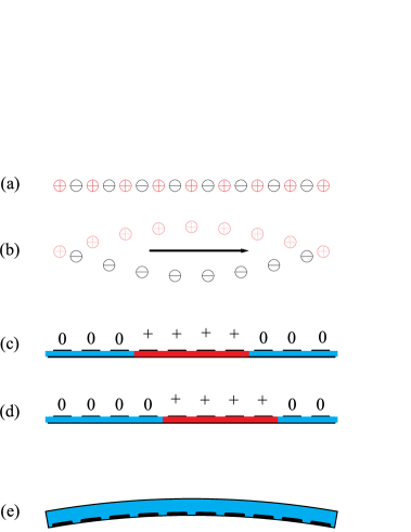
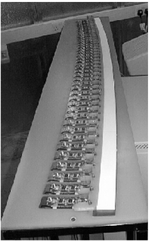
Figure 1: Left: experimental animation of a superluminal polarization current. (a) A simplified dielectric solid containing negative ($\ominus$) and positive ($\oplus$) ions. In (b), a spatially-varying electric field has been applied, causing the positive and negative ions to move in opposite directions; a finite polarization P has therefore been induced. If the spatially-varying field is made to move along the direction of the arrow, the polarized region moves with it. (c) Schematic side view of a practical superluminal source, showing metal electrodes above a strip of dielectric (shaded region) and a ground plate below it. “0” indicates that there is no voltage on that particular upper electrode; the symbol + indicates a positive voltage applied to the upper electrode. The voltage on the electrodes produces a finite polarization of the dielectric (darker shading). (d) By switching the voltages on the electrodes on and off, the polarized region (darker shading) can be made to move along the dielectric. (e) Top view, showing the curvature of the dielectric (lighter shaded region). The curvature introduces centripetal acceleration in the moving polarized region. Note also that the electrodes (black shading) cover only part of the top surface of the dielectric. In the discussion that follows, we refer to this section of the source (electrodes, dielectric and groundplate) as the “array”, for convenience. Right: a photograph of the experimental array; the copper shields have been removed from the 41 amplifiers so that their components are visible.

Symbol	Definition
$\omega$	Angular rotation frequency of the distribution pattern of the source.
$\Omega$	The angular frequency with which the source oscillates (in addition to moving).
	One of the two angular frequencies used to drive the experimental source (Eq. 3).
$f,~{}f_{\pm}$	Frequency of the radiation generated by the source; $f_{\pm}=|\Omega\pm m\omega|/2\pi$.
$n=2\pi f/\omega$	The harmonic number associated with a particular radiation frequency.
$m$	The number of cycles of the sinusoidal wave train representing the azimuthal
	dependence of the rotating source distribution [see Eq.2] around the
	circumference of a circle centred on, and normal to, the rotation axis.
$\eta=m\omega$	The second of the two angular frequencies used to drive the experimental source (Eq 3).

Table 1: Definition of the various frequencies and numbers used to describe the source and the emitted radiation, after Refs. [12, 13].

Thus far, the bulk of the theoretical analysis of superluminal light sources has been carried out for rotating, oscillating polarization current distributions [12, 13], which possess a polarization given (in cylindrical polar coordinates) by [23]

$${\bf P}(r,\varphi,z,t)={\bf s}(r,z)\cos[m(\varphi-\omega t)]\cos\Omega t.$$ (2)

Here s is a vector field describing the orientation of the polarization; it vanishes outside the active volume of the source [12]. The other parameters are defined in Table 1. The experimental superluminal source described in this paper represents a discretized version of Eq. 2. It consists of a continuous strip of alumina (i.e. the material to be polarized by the applied electric field) on top of which is placed an array of metal electrodes; underneath is a continuous ground plate. This forms what is in effect a series of capacitors (a schematic is shown in Fig. 1(c)-(e)). Each upper “capacitor” electrode is connected to an individual amplifier; turning the amplifiers on and off in sequence moves a polarized region along the dielectric (Fig. 1(c)-(d)).

In practice, the dielectric in the experimental source is a strip corresponding to a $10^{\circ}$ arc of a circle of average radius $a=10.025$ m, made from alumina 10 mm thick and 50 mm across. Above the alumina strip, there are 41 upper electrodes of mean width 42.6 mm, with centers 44.6 mm apart. Whilst the ground plate is the same width as the dielectric strip, each electrode covers only the inner 10 mm of the upper surface (shown schematically in Fig 1(e)). This has the effect of producing a polarization in the alumina with both radial and vertical components (see Eq. 2). In the discussion that follows, we shall refer to the assembly consisting of groundplate, dielectric and electrodes as “the array” for convenience.

Each upper electrode of the array is driven by an individual shielded amplifier just behind it; to simulate Eq. 2, the $j$th ($j=1$, 2, 3….) electrode is supplied with a voltage

$$V_{j}=V_{0}\cos[\eta(j\Delta t-t)]\cos\Omega t.$$ (3)

Comparison with Eq. 2 shows that the angular frequency $\eta=m\omega$; $\Delta t=\Delta\varphi/\omega$, where $\Delta\varphi=\pi/(18\times 40)$ is the angle subtended by the effective center separation of adjacent electrodes. The velocity $v$ with which the polarization current distribution propagates along the dielectric is set by adjusting $\Delta t$ to give $v=a\Delta\varphi/\Delta t$ (see Fig. 2(a)). Given the dimensions of the experimental array, $v>c$ is achieved for $\Delta t<148.8$ ps. (At this point it should be stated that the modulation scheme used to animate the superluminal polarization current is quite distinct from any used thus far in conventional phased-array antennae [19].)

The application of the electrode voltages produces a stepped approximation to a sinusoidal polarization-current wave that moves at speed $v$ along the dielectric (see Fig. 2(a)). Detailed analysis of this type of waveform (see Ref. [12], Appendix) shows that the dominant emission is almost identical to that produced by a pure sinusoidal wave with the same wavelength and amplitude. Most of the emission occurs at two frequencies, $f_{\pm}=|\Omega\pm\eta|/2\pi\equiv|\Omega\pm m\omega|/2\pi$, as indicated in Table 1.

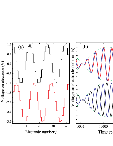
Figure 2: (a) The upper curve shows the instantaneous values of the voltages on the 41 upper electrodes of the array; $\eta/2\pi=552.653$ MHz and $\Delta t=140$ ps, corresponding to $v\approx 1.064c$ for $a=10.025~{}$m and $\Delta\varphi=\pi/(18\times 40)$ (see Eq. 3). The resulting polarizations under the electrodes will be proportional to these voltages. The lower curve (offset for clarity) gives the instantaneous voltages 420 ps later; the polarization “wave” has moved along the dielectric. (Note that the $\cos\Omega t$ term in Eq. 3 hardly changes during this time.) (b) Example of the time-dependent voltages on array electrodes 20 and 21 (upper curves) and 20 and 26 (lower curves) for the same parameters as in (a). Note that the lower-frequency temporal modulation of each electrode voltage produced by the second cosine term in Eq. 3 (dotted curves) is in phase for all electrodes.

As mentioned above, the speed of the source (i.e. the speed at which the sinusoidal polarization current “wave” propagates along the dielectric) is set by the parameter $\Delta t$. Experimentally, this is done by observing the time dependence of the voltages on each electrode (Figure 2(b)) using a high-speed oscilloscope.

Finally, it should be emphasised that great care was taken to minimize unwanted radiation from the amplifiers, cabling and signal generators of the apparatus to ensure that the detected signal was dominated by the emission from the polarization current. Steps taken included proper encasing of all of the signal generation equipment, the enclosure of the 41 amplifiers inside thick copper shields (not shown in Fig. 1) and the correct impedance matching of connections.

II.2 The experimental geometry

To map out the spatial distribution of the radiation from the superluminal source, one would ideally position the array in empty space and move a detector to points around it, covering a comprehensive range of angles and distances. However, practical experiments must be conducted close to the earth’s surface, where reflections from the ground are a complicating factor [14] (see Appendix); numerous tests showed that highly reproducible data are obtained when the “ground” under the path between array and detector is smooth, level and of a uniform quality [20]. After trials at several locations, the bituminised macadam surface of an airfield runway (Turweston Aerodrome, near Northampton, UK) was found to be almost ideal in providing a substantial length of well-characterized surface. All of the experiments reported in the current paper employ the runway, which is approximately 900 m long and 20 m wide. A change in slope about two-thirds of the way along the runway restricts the range tests reported in Section IV to distances of 600 m or less. However, measurements of the angular distribution of the radiated power from the array (Section III) employed the full length of 900 m.

The geometry of the runway dictates that the best configuration for measuring the spatial and angular distribution of the radiation is to fix the position of the detector (on the runway, at a distance $R$ from the source) and to change the orientation of the array to access a full range of polar and azimuthal angles. This is accomplished by placing the array on a platform that tilts about a horizontal-axis pivot at one end; this is in turn fixed on a turntable that can rotate about a vertical axis.

It is possible to mount the array on the platform in two configurations. In the first, the array plane is vertical (Fig. 3(a)), so that its long axis can be tilted (about the horizontal pivot) to an angle $\phi_{\rm V}$ with respect to horizontal; the turntable is then rotated about a vertical axis so that the array plane makes an angle $\vartheta_{\rm V}$ (in the horizontal plane) with the line connecting the detector at P and the array center. In the second configuration, the array plane is initially horizontal (Fig. 3(b)); the array plane is then tilted using the horizontal pivot to an angle $\vartheta_{\rm H}$ with respect to horizontal. The turntable is then rotated about a vertical axis so that the projection of the long axis of the array on the horizontal plane makes an angle $\phi_{\rm H}$ with the line connecting the detector at P and the array center.

Finally, to aid comparison of experiment and theory, it is necessary to relate the experimental spherical polar coordinates $(R,\vartheta_{\rm V},\phi_{\rm V})$ and $(R,\vartheta_{\rm H},\phi_{\rm H})$, which are measured relative to the array center, to the cylindrical and spherical polar coordinates used to evaluate the integrals in the Appendix and in Refs. [12, 13]. In the latter papers, each volume element of the superluminal source distribution traverses a complete circular orbit centered at the origin of the coordinate system, and the radial distances to the individual source elements and to the observation point at $(R_{\rm P},\theta_{\rm P},\varphi_{\rm P})$ are specified with respect to the common center of these circular orbits (see Fig. 3(c) and (d)). Although the experimental source does not encompass a complete circle, the high degree of symmetry represented by this coordinate system greatly facilitates the computation of the integrals in the Appendix. The relationship between the experimental coordinates and the coordinate system used in the Appendix is shown in Figs. 3(c) and (d).

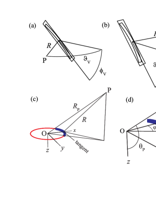
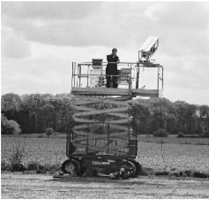
Figure 3: Left: the coordinates used to measure the spatial distribution of radiation from the array. In the experiments ((a),(b)), the detector is at a fixed point P, distance $R$ from the array; the array is placed on a platform tilting about a horizontal axis pivot that is in turn fixed to a turntable rotating about a vertical axis. In (a), the array plane is vertical; its long axis is tilted to an angle $\phi_{\rm V}$ with respect to horizontal. The turntable is rotated about a vertical axis so that the array plane makes an angle $\vartheta_{\rm V}$ (in the horizontal plane) with the line connecting P and the array center. In (b), the array plane is initially horizontal; the array plane is then tilted to an angle $\vartheta_{\rm H}$ with respect to horizontal. The turntable is rotated about the vertical axis so that the projection of the long axis of the array on the horizontal plane makes an angle $\phi_{\rm H}$ with the line connecting P and the array center. Note that the coordinate systems are not equivalent; $\tan\phi_{\rm V}=\tan\phi_{\rm H}/\cos\vartheta_{\rm H}$ and $\sin\vartheta_{\rm V}=\sin\vartheta_{\rm H}\cos\phi_{\rm H}$. (c) The array and detector positions in terms of the coordinate system used in the Appendix and Refs. [12, 13]. In the model, each volume element of the sourse moves on a circular path centered at the origin O; a typical path is shown, with the array being represented by thicker shading. The array center is at $(a,0,0)$, and the tangent to the array is parallel to the $y$ axis; the distances, from O, to the detector ($R_{\rm P}$) and to the array center ($R$) are compared. (d) Definition of the spherical polar coordinates $R_{\rm P},\theta_{\rm P},\varphi_{\rm P}$ used in the Appendix. The arrow indicates the direction of propagation of the polarization current distributions in the experimental array. Right: the array in use during the experiments.

II.3 Detector system, array and detector heights, and interference from ground reflections

The detector was a Schwarzbeck Mess-Elektronik UHA 9105 half-wave tuned dipole antenna, optimized for the frequency range 300 MHz to 1 GHz. and mounted on a mobile wooden tower that allowed it to be fixed at varying heights $h_{\rm D}$ above the ground. The antenna was fitted with an internal coaxial BAL-UN to ensure good impedance matching with an external load and was connected via a 6 m long impedance-matched coaxial cable ($50~{}\Omega$) to an Anritsu MS2711B portable spectrum analyser. The background noise floor with this equipment was between -120 and -130 dBm, depending on weather conditions at the airfield.

In the current paper, the settings of the experimental machine are such that the emitted radiation is polarized chiefly in directions parallel to the plane of the array. When the array is orientated as in Fig. 3(a), the detector aerial (see below) is arranged to detect vertically-polarized radiation; if the array is orientated as in Fig. 3(b), the detector is configured to detect horizontally-polarized radiation.

For the measurements described in the following sections, the array turntable was mounted on a scissor lift that allowed the height of the center of the array above the runway to be varied between $h_{\rm A}=3.3$ m and 5.0 m; for each measurement, the heights $h_{\rm A}$ and $h_{\rm D}$ were measured to an accuracy of $\pm 5$ cm. An accurate measurement of $h_{\rm A}$ and $h_{\rm D}$ is important because the intensity received at the detector results from interference between signals traveling along a direct path between array and detector and reflections from the ground [14]. The situation is shown in Fig. 4(a). This process is covered in detail in the Appendix.

The effect of the interference on the signal received from a simple horizontally-polarized dipole aerial is shown in Fig 4(b). Firstly, clear fringes are seen in the detected intensity as a function of distance. A second consequence of the interference is less obvious. Fig. 4 shows received power in the logarithmic units Belm versus $\log_{10}$(distance); the gradient of the plot should be $-\gamma$, where (received power) $\propto$ (distance)^-γ. Naive expectations based on the emission of a dipole surrounded by infinite empty space lead one to predict $\gamma=2$ (the inverse square law [15]); in practice, the interference leads to $\gamma\approx 4$ (see Fig. 4(b)). Such a dependence is familiar to radio engineers as the penultimate term of the “Egli” relationship [21] describing the power lost for frequencies $f$ in the hundreds of MHz range when transmitting over a path close to the earth’s surface:

$${\rm path~{}loss~{}(dB)}=113+20\log_{10}f+40\log_{10}({\rm path~{}length~{}(miles)})-20\log_{10}(h_{\rm A}h_{\rm D}).$$ (4)

The effects of interference obviously complicate the search for the non-spherical decay associated with the cusp (see Section IV). One criterion used in the experiments was to look for significantly smaller path losses than Egli (Eq. 4); more detailed analysis was then used to model the detailed behavior of the data.

Reflections from the ground complicate also the modeling of the angular distribution of the emission from the array. A detailed treatment of the coordinates needed for delineating the direct and reflected rays is given in the Appendix, as are the equations from Refs. [12, 13] required for modeling the data.

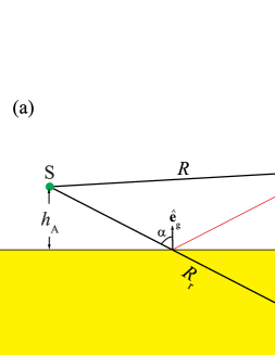
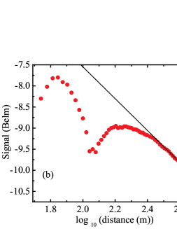
Figure 4: (a) Geometry of the interference between a direct wave from the source S, height $h_{\rm A}$ above the ground, and a wave reflected from the ground. The detector, at height $h_{\rm D}$ above the ground, is labeled by P. The direct waves travel a path length denoted by $R$. The path source-ground-detector is equal in length to a direct path from the source to an image of P at P^′. The length of this equivalent path is denoted by $R_{\rm r}$. The other symbols shown are used in the Appendix. (b) Effect of interference on the power received from a horizontally-polarized dipole aerial excited at $598.696$ MHz as a function of distance ($h_{\rm A}=5.12$ m; $h_{\rm D}=5.0$ m). The points are data, and the straight line is a least-squares fit to the data beyond the final interference fringe; the gradient is $\gamma=-3.8$.

III Experimental results: intensity distribution of the radiation

III.1 Intensity as a function of $\vartheta_{\rm V}$ at fixed $\phi_{\rm V}$

The array was mounted in the configuration shown in Fig. 3(a) and the detector antenna placed at a fixed distance $R$ away; detector and array were fixed at heights $h_{\rm D}$ and $h_{\rm A}$ respectively above the level runway. The angle $\phi_{\rm V}$ was set to a series of fixed values with an accuracy of $\pm 0.5^{\circ}$ using a Suunto clinometer, and then the angle $\vartheta_{\rm V}$ was varied using the turntable. The measurement of $\vartheta_{\rm V}$ was made to an accuracy of $\pm 0.5^{\circ}$ using a graticule on the turntable. At each value of ($\vartheta_{\rm V},\phi_{\rm V}$), the intensity of the signal at the detector antenna was measured using the spectrum analyser.

Fig. 5(a) shows the effect of varying the source speed $v=a\Delta\varphi/\Delta t$ on the intensity distribution as a function of $\vartheta_{\rm V}$. Data for $v/c=1.064$, 1.25 and 2.0 are shown; for each data set, $\eta/2\pi=552.654$ MHz, $\Omega/2\pi=46.042$ MHz, and the observation is made at the higher of the two emitted frequencies, $f_{+}=|(\Omega+m\omega)|/2\pi\equiv(\Omega+\eta)/2\pi=598.696$ MHz. As the source speed increases, the peak in detected power moves out to higher values of $\vartheta_{\rm V}$, in line with expectations; the contributions that are received from different source elements, by an observer in the far field, are in phase when (see Appendix, Eqs. 23 and 50)

$$\theta_{\rm P}=\arcsin\Big{(}{{mc}\over{nv}}\Big{)},\quad{\rm or}\quad\vartheta_{\rm V}=\arcsin\Big{\{}{R\over R_{\rm P}}\Big{[}1-\Big{(}{{mc}\over{nv}}\Big{)}^{2}\Big{]}^{1\over 2}\Big{\}}.$$ (5)

Here $n=2\pi f/\omega$ is the harmonic number of the emitted radiation with $f=f_{+}$ or $f_{-}$, and $m=\eta/\omega$ is determined by the angular frequency $\omega=v/a=\Delta\varphi/\Delta t$ of the rotation of the source (see Table 1) [12]. Note that the data are well reproduced by the model (see Appendix, Eq. 47) using the experimental source speeds.

Compared to the emission of a conventional antenna [25], the rather small side lobes are a further characteristic of the beaming produced by an accelerated superluminal source. To show this more clearly, a single data set, corresponding to $v/c=2.0$, is shown in Fig. 5(b). Although the projection of the length of the array onto a plane normal to the observation direction is comparable to or smaller than the radiation wavelength and the observation is made at many hundreds of Fresnel distances, most of the power is transmitted in a beam around $20^{\circ}$ wide, with small side lobes. This beam structure is reproduced very well by the model (Appendix, Eq. 47), using the experimental source speed as an input parameter. (In the case of the present emission mechanism, the side lobes are caused mainly by interference from the ground; it follows from Eq. 47 that in free space they would be much weaker.)

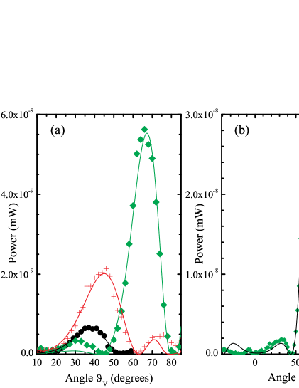
Figure 5: (a) The effect of varying the source speed, $v=a\Delta\varphi/\Delta t$ on the angular distribution of the radiation from the array. For each data set, $\phi_{\rm V}=2^{\circ}$ and the array to detector distance is $R=600$ m. Data are points, identified as follows: filled circles: $v=1.064c$, $h_{\rm A}=3.7$ m, $h_{\rm D}=4.1$ m; crosses: $v=1.25c$, $h_{\rm A}=h_{\rm D}=5.0$ m; diamonds: $v=2.0c$, $h_{\rm A}=h_{\rm D}=5.0$ m. The curves are fits, using the model (Eq. 47) described in the Appendix. For each data set, $\eta/2\pi=552.654$ MHz, $\Omega/2\pi=46.042$ MHz, and the observation is made at the higher of the two emitted frequencies, $f_{+}=|(\Omega+m\omega)|/2\pi\equiv(\Omega+\eta)/2\pi=598.696$ MHz. Note that the peak emission moves out to higher values of $\vartheta_{\rm V}$ as the source speed increases. (b) Power detected versus $\vartheta_{\rm V}$ over a wider angular range than (a); here, $R=400$ m, $h_{\rm A}=h_{\rm D}=5.0$ m, $\phi_{\rm V}=2^{\circ}$ and the frequency is the same as in (a). The points (hollow diamonds) are data; the model (using the experimental source speed) is the continuous curve.

Whilst Fig. 5 shows data for the emission at $f_{+}=|(\Omega+\eta)|/2\pi$, the description of the source, Eq. 2, leads one to expect simultaneous emission at a second frequency, $f_{-}=|(\Omega-\eta)|/2\pi$. As $f_{+}$ and $f_{-}$ have different harmonic numbers, $n$, their angle of emission will differ slightly (see Eq. 5 and Table 1). This effect is shown for source speeds of $v/c=2.0$ in Fig. 6(a) and $v/c=1.25$ in Fig. 6(b). In each case, the emission at $f_{+}$ is peaked at a higher value of $\vartheta_{\rm V}$ than that at $f_{-}$, as predicted by Eq. 5 and the solid curves (see Appendix).

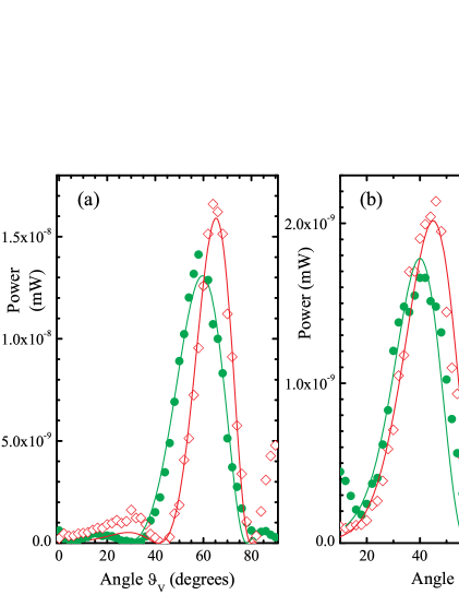
Figure 6: Comparison of the emission at $f_{+}=(\eta+\Omega)/2\pi=598.696$ MHz (hollow diamonds) or $f_{-}=(\eta-\Omega)/2\pi=506.614$ MHz (filled circles) for two different source speeds. In (a), $v=2.0c$, $R=400$ m, $h_{\rm A}=3.32$ m, $h_{\rm D}=3.71$ m and $\phi_{\rm V}=2.5^{\circ}$. In (b), $v=1.25c$, $h_{\rm A}=h_{\rm D}=5.0$ m, $\phi_{\rm V}=2^{\circ}$ and $R=600$ m. For all data sets, the values of $\Omega$ and $\eta$ are the same as those in Fig. 5, and in all cases the curves are generated by the model (Eq. 47) using the experimental values of $f_{\pm}$ and $v/c$. Note that, in agreement with Eq. 5, the emission is peaked at higher values of $\vartheta_{\rm V}$ for $f_{+}$ than for $f_{-}$.

It has already been mentioned in the discussion of Fig. 5(a) that the beam is rather sharply defined as a function of $\vartheta_{\rm V}$, even though the projection of the length of the array on the plane perpendicular to the observation direction is comparable to or smaller than the radiation wavelength. This characteristic is independent of distance over the range measured, as shown in Fig. 7, which plots data (points) for $200~{}{\rm m}\leq R\leq 900$ m. For all of these $R$ values, each representing hundreds of Fresnel distances, the central part of the beam preserves its overall width and general shape. This development of beam structure with $R$ is reproduced by the theoretical description (Fig. 7, curves; see Appendix, Eq. 47), using the experimental source speed as input parameter.

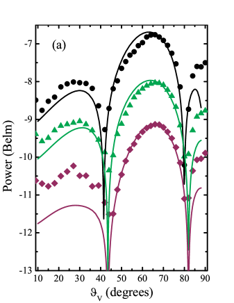
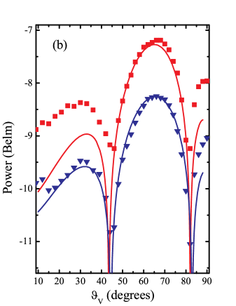
Figure 7: (a) The $\vartheta_{\rm V}$ dependence of the detected power for $R=200~{}{\rm m}$ (circles), $500~{}$m (triangles), and $900~{}$m (diamonds). (b) The $\vartheta_{\rm V}$ dependence of the detected power for $R=300~{}$m (squares) and $600~{}$m (inverted triangles). In both cases, $f_{+}=(\eta+\Omega)/2\pi=598.696$ MHz, $v=2.0c$, $h_{\rm A}=h_{\rm D}=5.0$ m and $\phi_{\rm V}=2^{\circ}$; points are data and curves are fits to the model in the Appendix (Eq. 47).

Note that all of the data sets plotted in this Section involve small values of $\phi_{\rm V}(\sim 2^{\circ})$. The reason for this constraint is that as well as having a peaked structure as a function of the polar angle $\vartheta_{\rm V}$, the emission of the source is also peaked in the plane of rotation (i.e. around $\phi_{\rm V}=\phi_{\rm H}=0$), as expected in the theoretical description [12, 13]. This observation will be described in the following Section.

III.2 Intensity as a function of $\phi_{\rm H}$ at fixed $\vartheta_{\rm H}$

The array was mounted in the configuration shown in Fig. 3(b) and the detector was placed at a fixed distance $R$ away; detector and array were fixed at the respective heights of $h_{\rm D}$ and $h_{\rm A}$ above the level runway. The angle $\vartheta_{\rm H}$ was set to a series of fixed values to an accuracy of $\pm 0.5^{\circ}$ using a Suunto clinometer, and then the angle $\phi_{\rm H}$ was varied using the turntable. The measurement of $\phi_{\rm H}$ was carried out using a graticule on the turntable to an accuracy of $\pm 0.5^{\circ}$. At each value of ($\vartheta_{\rm H},\phi_{\rm H}$) the intensity was recorded.

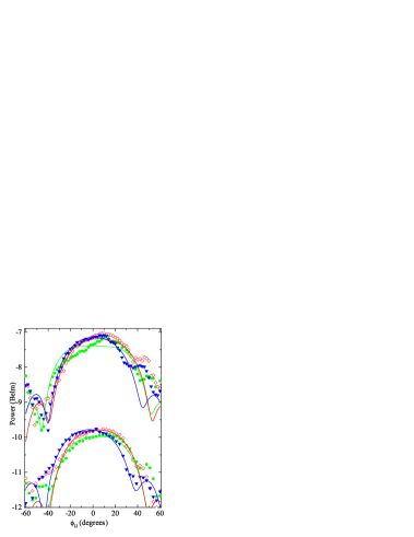
Figure 8: The $\phi_{\rm H}$ dependence of the detected power (logarithmic scale) for $R=200~{}{\rm m}$ (upper) and 900 m (lower) for $\vartheta_{\rm H}=30^{\circ}$ (filled circles), $35^{\circ}$ (hollow diamonds) and $40^{\circ}$ (inverted triangles). Solid curves are fits to the model in the Appendix (Eq. 47). The frequency is $f_{+}=(\eta+\Omega)/2\pi=598.696$ MHz, $v=1.064c$, $h_{\rm A}=h_{\rm D}=5.0$ m.

Fig. 8 shows the beam profile as a function of $\phi_{\rm H}$ for $\vartheta_{\rm H}=30^{\circ}$, $35^{\circ}$ and $40^{\circ}$ and distances $R=200$ m and 900 m. Note that the peak emission is centered around $\phi_{\rm H}=0$, as expected from theory [12]; variations of $\phi_{\rm H}$ of around $\pm 10^{\circ}$ away from zero do not affect the intensity much, but thereafter, the intensity falls away rapidly.

Taken in conjunction with Fig. 5, the data in Fig. 8 show that the emission from the superluminal source is tightly beamed in both the azimuthal and polar directions. The observation of a peaked emitted power distribution (see Fig. 6) at two frequencies shows that this effect is frequency independent, depending instead on the speed of the source and the geometry of the array. Once again we contrast this with the case of a conventional antenna [25]; the beaming occurs even though the projection of the length of the array onto a plane normal to the observation direction is comparable to or smaller than the radiation wavelength and the observation is made at many hundreds of Fresnel distances.

Finally, we remark that the evolution of the beam profile as $\vartheta_{\rm H}$ and $\phi_{\rm H}$ vary is in good agreement with the expectations of theory [12]. Fig. 9 shows the the $\phi_{\rm H}$ dependence of the detected power (linear scale) for several values of $\vartheta_{\rm H}$. The evolution of the beamshape, including the development of a precursor (a side maximum), is well reproduced by the model (Appendix, Eq. 47), using the experimental value of $v/c$.

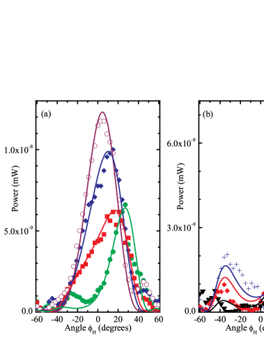
Figure 9: (a) The $\phi_{\rm H}$ dependence of the detected power (linear scale) for $\vartheta_{\rm H}=40^{\circ}$ (hollow circles), $35^{\circ}$ (filled diamonds), $30^{\circ}$ (filled squares) and $25^{\circ}$ (filled circles). Points are data; the curves are the model (Eq. 47) predictions. (b) The $\phi_{\rm H}$ dependence of the detected power for $\vartheta_{\rm H}=20^{\circ}$ (inverted triangles), $15^{\circ}$ (diamonds) and $10^{\circ}$ (crosses). Points are data; the curves are the model predictions (Eq. 47). In both (a) and (b) $R=400$ m, the frequency is $f_{+}=(\eta+\Omega)/2\pi=598.696$ MHz, $v=1.06c$, $h_{\rm A}=h_{\rm D}=5.0$ m.

IV Nonspherically decaying component of the radiation

IV.1 General properties

The previous section has shown that the angular distribution of the emission from the experimental source is in good quantitative agreement with theoretical predictions for a rotating, oscillating superluminal source (see Appendix) [12, 13]. However, the most controversial aspect of the model of Refs. [6, 12, 13] has been the prediction of a component of the emission that decays nonspherically, i.e. as $1/R$, rather than $1/R^{2}$ [7, 8]. This component is due to an effect, only possible in the case of an accelerated superluminal source, whereby waves that were emitted over a finite interval of emission time arrive at the detector during a much shorter interval of reception time. The constructive interference of such superposed waves is strongest if their emission time interval is centered at the instant at which their source approaches the detector (along the radiation direction) with the wave speed (the speed of light) and zero acceleration. The locus of the series of points for which this occurs for a single volume element of the source constitutes the propagating space curve which we have here called the cusp [6, 13].

In this section, we describe the location and the characteristic features of this emission for a source speed of $v=1.064c$ and the frequency $f_{+}=(\Omega+\eta)/2\pi=598.696$ MHz; the theoretical predictions for this speed lead one to expect that the cusp loci will be found close to $\vartheta_{\rm H}=20^{\circ}$ at small values of $\phi_{\rm H}$: For a source that is centered at $\varphi=0$ and an observation point that lies in the far field, Eq. 49 of Ref. [13] reduces to $\varphi_{\rm P}\simeq-3\pi/2$, $\theta_{\rm P}\simeq\arcsin[c/(r\omega)]$, in which $r\omega\equiv v$.

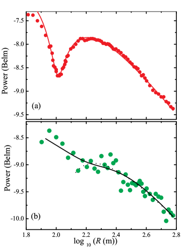
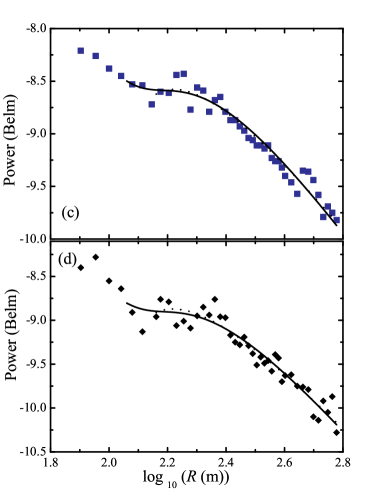
Figure 10: (a) Detected power (logarithmic scale) versus $\log_{10}(R)$, where $R$ is the array-to-detector distance for a subluminal source, velocity $v/c=0.875$; $h_{\rm A}=h_{\rm D}=5.0$ m, $\phi_{\rm H}=0$, $\vartheta_{\rm H}=35^{\circ}$, $f_{+}=(\eta+\Omega)/2\pi=598.696$ MHz. The points are data; the curve is the interference model described in the Appendix; the refractive index is $N=1.074$. (b) Detected power versus $\log_{10}(R)$ for the superluminal source close to the expected cusp direction. The source velocity is $v/c=1.064$, $h_{\rm A}=h_{\rm D}=5.0$ m, $\phi_{\rm H}=-5^{\circ}$, $\vartheta_{\rm H}=20^{\circ}$, $f_{+}=(\eta+\Omega)/2\pi=598.696$ MHz. Data are points; the dotted curve is a fit to Eq. 17 (Appendix). This model is valid for larger $R$ and assumes both no beaming and an intensity proportional to $1/R^{2\kappa}$. Fit parameters are $2\kappa=0.90$ and $N=1.074$. The solid curve represents a fit to Eqs. 18 and 19 that uses a Gaussian beam of width $2w$; fit parameters are $2\kappa=1.05$, $2w=4.18^{\circ}$ and $K=16.6$. (c) Detected power versus $\log_{10}(R)$ to one side of the cusp direction; all experimental details are the same as in (b) except $\phi_{\rm H}=0$. Data are points, the dotted line is a fit to Eq. 17 ($2\kappa=1.41$, $N=1.074$). The solid curve is a fit to Eqs 18 and 19 ($2\kappa=1.47$, $2w=6.69^{\circ}$, $K=17.3$). (d) Same as (c) but with $\phi_{\rm H}=-10^{\circ}$. Data are points; the fit to Eq. 17 is dotted ($2\kappa=1.47$, $N=1.074$). the solid curve is a fit to Eqs 18 and 19 ($2\kappa=1.48$, $2w=6.56^{\circ}$, $K=14.6$). (The data shown here are limited to $R\leq 600$ m because the runway at the Turweston Aerodrome dips sharply in its last $300$ m.)

As a reference point, Fig. 10(a) shows the detected power versus array-to-detector distance $R$, both plotted on logarithmic scales, for the case of the source moving subluminally; the velocity is $v/c=0.875$. Note that the data (points) are very similar to those shown in Fig. 4 for the emission of a dipole aerial; indeed, the data are well fitted using the interference model for a point-like source and spherical decay described in the Appendix (curve), especially at larger distances where the finite array size is much smaller than $R$. This suggests that the emission of the array running subluminally is entirely “conventional”; the detected power obeys the inverse square law (once the effects of interference are taken into account), and at large distances the source appears point-like.

Figure 10(b) shows detected power versus $\log_{10}(R)$ for the source running superluminally ($v/c=1.064$), for array-to-detector distances $R$ measured along the expected direction of the cusp loci. The contrast with Fig. 10(a) is immediately visible, and involves three distinct differences:

1. The interference fringe visible at around $\log_{10}(R)=2$ in (a) is absent in (b).

2. At larger distances, the detected power falls off with distance more slowly in (b) than in (a).

3. The data in (b) possess a much greater “scatter” than those in (a). This scatter occurs in spite of the fact that the detected power is $\sim 50$ dB above the noise floor; moreover, the scatter is to a large extent reproducible.

The last point can be understood by noting that the cusps represent emission by those volume elements of the source that travel towards the detector at zero acceleration and the speed of light, volume elements that collectively function as a coherent source [13]. The power emitted by a coherent source (such as a laser) normally contains reproducible variations known as “speckle” [24]; the reproducible scatter seen in Fig. 10(b) is due to just such a phenomenon.

Turning to the other differences between Fig. 10(a) and (b), the absence of an interference fringe is expected if the radiation along this direction is tightly beamed (the loci of the cusps are expected to have narrow angular width [12, 13]), so that it is not reflected from the ground close to the array; a detailed treatment of this effect is given in the Appendix (Eqs. 18 and 19). The slower decrease in power with increasing distance is another consequence of the properties of the cusps; we shall return to the exact exponent describing the decrease below.

Figure 11: (a) and (b): Ratio ${\cal P}^{\rm cusp}/{\cal P}^{\rm sub}$ (see Eq. 9) of the detected power with the source running superluminally (at $v/c=1.064$) to that with the source running subluminally ($v/c=0.875$) versus $R$, measured on two separate occasions. Both data sets follow paths close to the expected direction of the cusps; $h_{\rm A}=h_{\rm D}=5.0$ m, $\phi_{\rm H}=-5^{\circ}$, $\vartheta_{\rm H}=20^{\circ}$, $f_{+}=(\eta+\Omega)/2\pi=598.696$ MHz. Data are points; the lines are fits to Eq. 6 with $\mu\approx 1$. A linear fit through the origin implies that the power in the superluminal case would decline in free space as $1/R$ (see Eq. 9). (c) and (d) show similar plots just off the cusp direction; $\varphi_{\rm H}=0$ in (c), and $\varphi_{\rm H}=-10^{\circ}$ in (d). All other parameters are the same as in (a) and (b). The fits (solid curves) are to Eq. 6 with $\mu=0.62$ in (c) and $\mu=0.52$ in (d); i.e. the power ratio increases more slowly with distance, and cannot be fitted with a line through the origin.

As mentioned above, the cusps occupy only a small angular range; morover, they are expected to become narrower, the further one goes from the source. Some idea of this effect is gained by rotating the array by $5^{\circ}$; whereas Fig. 10(b) has $\phi_{\rm H}=-5^{\circ}$, Figs. 10(c) and (d) show similar data for $\phi_{\rm H}=0$ and $\phi_{\rm H}=-10^{\circ}$ respectively. Note that the small shift in direction has resulted in data that exhibit a smaller degree of “scatter” compared to those in Fig. 10(b) (especially at larger $R$), and that the detected power falls off more rapidly with increasing distance in (c) and (d) than in (b). The first observation is entirely expected; once one is off the cusp loci, the source no longer appears as coherent [13], and so the “speckle” effects should decrease. Along directions that appreciably differ from that of the cusp loci, the emitted power has the same dependence on distance as in Fig. 10(a), i.e. as in the case of a subluminal source or a conventional dipole.

Having identified the distinct features of the non-spherically-decaying component of the radiation, we describe in the following sections three experimental methods for determining the exponent $2\kappa$ that describes the rate at which the intensity of this component decays with distance $R$ (i.e. intensity $\propto 1/R^{2\kappa}$). In each case, we shall find that $2\kappa\approx 1$, in agreement with theoretical expectations [6, 13].

IV.2 Determination of the rate at which power falls off with distance using models of the interference

Comparison of Figs. 10(a)-(d) shows that the detected power decreases most slowly with increasing distance in the case of superluminal velocities and measurements along the cusp direction (Fig. 10(b)). However, obtaining the exponent $2\kappa$ for this decrease is complicated by the effects of interference from the ground; we have already seen that even the emission of a simple dipole does not decrease as $1/R^{2}$ (Fig. 4(b)) in proximity to the ground. The part of the radiation corresponding to the cusps provides a further complication in that it is expected to be tightly beamed [6, 13]; the current experimental machine agrees with these predictions in that the beam width of of the non-spherically-decaying component is appreciably (by an order of magnitude or more) narrower than the beams observed in the spherically-decaying part of the radiation (as shown in Figs. 5-9). A narrow beam will not be appreciably reflected from the ground when the detector is close to the array; hence, features due to interference will be suppressed.

Two treatments for this problem are included in the Appendix (Eqs. 17 to 19). If the beam has an angular spread $2w$, then at distances $R~{}\mbox{{\raisebox{-1.72218pt}{$\stackrel{{\scriptstyle>}}{{{\scriptstyle\sim}}}$}}}~{}h_{\rm A}/w$, a substantial proportion of the beam will be reflected from the ground; therefore a relatively simple treatment of interference (Eq. 17) can be used. The only input parameters are the power law of the decay of the radiation with distance (intensity $\propto 1/R^{2\kappa}$) and $N$, the refractive index of the ground (already constrained to be $N=1.074$ by fitting the interference fringes of the subluminal emission–see Fig. 10(a)). This method (Fig. 10(b), dotted curve) yields a value $2\kappa=0.90$, i.e., an intensity proportional to $1/R^{0.90}$.

For smaller values of $R$, a more sophisticated fitting method (Appendix; Eqs. 18, 19) takes account of the beaming by using a Gaussian beam of angular width $2w$, and also allowing for the presence of residual spherically-decaying waves close to the array. This function is shown as a solid curve in Fig. 10(b); the fit parameters are $2\kappa=1.05$, $2w=4.18^{\circ}$ and $K=16.6$ (see Eq. 19). This implies that the non-spherically-decaying part of the radiation has an intensity that decays as $1/R^{1.05}$ and that it is confined to an angular width $\sim 4^{\circ}$. The fact that $K$, which depends on the geometry and perfection of the source, is substantially larger than 1 implies that the dominant emission from the experimental machine is spherically-decaying, with a small component of non-spherically-decaying emission.

The narrow angular width of the non-spherically-decaying part of the radiation is emphasised by Figs. 10(c) and (d), which show the detected power versus distance for $\phi_{\rm H}=0$ and $\phi_{\rm H}=-10^{\circ}$ (rather than the $\phi_{\rm H}=-5^{\circ}$ used in Fig 10(b)). The power falls off more quickly at large distances in (c) and (d) than in (b), and this is reflected in the fits. For example, in (c), the simple model (dotted curve; Eq. 17) yields $2\kappa=1.41$ (with $N$ constrained to be $1.074$ to match the fit in Fig. 10(a)), whereas the more sophisticated Eqs. 18 and 19 (solid curve) give $2\kappa=1.47$, $2w=6.69^{\circ}$ and $K=17.3$. Both fits suggest an intensity that is approximately $\propto 1/R^{1.5}$ and the latter is suggestive of less beaming of the radiation. Similar considerations apply to the fits to the data in Fig. 10(d).

IV.3 Determination of the rate at which power falls off with distance using intensity ratios

An alternative, model independent way of determining the exponent $2\kappa$ is to divide the power detected along the cusp by that detected when the source is run subluminally under similar conditions. Such a comparison can only be made beyond the region containing the interference fringes (i.e. $R>150$ m), because (as mentioned above) the cusp has a distinctly “beamed” character, whereas the radiation from the subluminal source is much more isotropic. This comparison is shown in Figs. 11(a) and (b) for data taken on two separate occasions with differing weather conditions. Each data set represents the detected power ${\cal P}^{\rm cusp}$ along the expected cusp direction with the source running superluminally ($v/c=1.064$), divided by the detected power ${\cal P}^{\rm sub}$ with the source running subluminally ($v/c=0.875$). In both subluminal and superluminal runs, all other experimental parameters were identical.

The data were fitted to a function

$$\frac{{\cal P}^{\rm cusp}}{{\cal P}^{\rm sub}}={\cal C}R^{\mu}$$ (6)

where $\mu$ and ${\cal C}$ are fit parameters. The fits yielded $\mu\approx 1$, i.e. a straight line through the origin, implying that the power ratio is roughly proportional to $R$ (Figs. 11(a), (b)). This result can be explained as follows. Once the interference fringes have been passed, ${\cal P}^{\rm sub}$ will obey an approximate relationship

$${\cal P}^{\rm sub}(R)\approx\frac{{\cal C}^{\rm sub}}{R^{~{}\nu}},$$ (7)

where ${\cal C}^{\rm sub}$ is a constant or a very slowly-varying function of $R$. There are many precedents for the use of such power laws in the empirical functions [14, 21, 22] for describing radio transmission (e.g. Eq. 4). The straight lines through the origin seen in Figs. 11(a),(b) will only occur if the power ${\cal P}^{\rm cusp}$ follows the relationship

$${\cal P}^{\rm cusp}\approx\frac{{\cal C}^{\rm cusp}}{R^{~{}\nu-1}},$$ (8)

so that

$$\frac{{\cal P}^{\rm cusp}}{{\cal P}^{\rm sub}}\approx\frac{{\cal C}^{\rm cusp}}{{\cal C}^{\rm sub}}R.$$ (9)

This again suggests that the power in the non-spherically-decaying component of the radiation would decay in free space more slowly with distance $R$ than $1/R^{2}$.

Once again, the narrowness of the region occupied by the cusps can be demonstrated by shifting $\phi_{\rm H}$ by only $5^{\circ}$ (Figs. 11(c),(d)). The power ratio increases more slowly with distance, and the data can no longer be fitted by a straight line through the origin; instead $\mu=0.62$ in (c) and $0.52$ in (d) (see Eq. 6).

IV.4 Summary

The various methods of characterizing the rate at which the detected power falls off with $R$ shown in Figs. 10 and  11 suggest that the intensity of the non-spherically-decaying component is roughly proportional to $1/R$, in agreement with theoretical predictions [6, 13]. Moreover, the relatively small angular range over which this $1/R$ dependence is observed (compare Figs. 10(b) and (c)) emphasises the narrowness of the region occupied by the cusps.

Note that in the present experiments, the Fresnel distance (Rayleigh range) is of the order of a few meters. The maximum length of the array that can be projected onto a plane perpendicular to the propagation direction is $l=1.74$ m and the shortest wavelength used is $\lambda=0.50$ m. These together yield a maximum Fresnel distance $R_{\rm F}=l^{2}/\lambda=6.0$ m. There is no parameter other than the Fresnel distance to limit the range of validity of the above results, and these, as we have seen, have been tested for $R\gg R_{\rm F}$.

V Conclusion

In summary, we have constructed and tested an experimental implementation of an oscillating, superluminal polarization current distribution that undergoes centripetal acceleration. Theoretical treatments [12, 13] lead one to expect that the radiation emitted from each volume element of such a polarization current will comprise a Čerenkov-like envelope with two sheets that meet along a cusp. The emission from the experimental machine has been found to be in good agreement with these expectations, the combined effect of the volume elements leading to tightly-defined beams of a well-defined geometry, determined by the source speed and trajectory. In addition, over a restricted range of angles, we detect the presence of cusps in the emitted radiation. These are due to the detection over a short time period (in the laboratory frame) of radiation emitted over a considerably longer period of source time. Consequently, the intensity of the radiation at these angles was observed to decline more slowly with increasing distance from the source than would the emission from a conventional antenna. The angular distribution of the emitted radiation and the properties associated with the cusp are in good quantitative agreement with theoretical models of superluminal sources once the effect of reflections from the earth’s surface are taken into account. In particular, the prediction that the beaming and the slow decay should extend into the far-zone has been tested to several hundred Fresnel distances.

The above results have implications not only for the interpretation of observational data on pulsars, which originally motivated the theoretical investigation of the present emission process [6, 10], but also for a diverse set of disciplines and technologies in which these findings have potential practical applications [26]. One such technology is long-range and high-bandwidth telecommunications.

Since all of the processes involved in generating the polarization current distribution are linear, and the direction of the emitted “beam” only depends on the source speed, it should be simple to use an array to broadcast several beams in different directions simultaneously. This could be achieved by applying voltages which are sums of terms like Eq. 3, each with a different speed, to the electrodes of an array. The beaming is frequency independent, and so an array could potentially be used to transmit multiple directed beams at several frequencies. (The very small side lobes, especially in free space, are a further characteristic of the beaming produced by the present emission mechanism that facilitates this type of transmission.)

Of particular practical significance are the properties of the non-spherically-decaying component of the radiation that we have observed: the fact that its intensity decays like $1/R$, rather than $1/R^{2}$, with the distance $R$ from its source, and that its beam-width is less than $\sim 5^{\circ}$ at $\sim 500$ m. This radiation mechanism could thus be used, in principle, to convey electronic data over very long distances with very much lower attenuation than is possible with existing sources. In the case of ground-to-satellite communications, for example, the above properties imply that either far fewer satellites would be required for the same bandwidth or each satellite could handle a much wider range of signals for the same power output.

The excellent correspondence between the experimental data and theoretical predictions supports the proposal that polarization current distributions act as superluminal sources of radiation, and that they can be used for studying and utilizing the novel effects associated with superluminal electrodynamics. The apparatus described in this paper represents just one possible geometry and excitation scheme. In principle, a whole class of superluminal sources are possible, corresponding, for example, to a rectilinearly accelerated polarization current [6] (rather than a centripetally accelerated one), or to a medium that is polarized by impinging laser beams (rather than by applied voltages), and so on. It is hoped that the publication of this paper will stimulate further work along these lines.

VI Acknowledgements

The experimental research was supported by the Engineering and Physical Sciences Research Council (UK), under grant GR/M52205/01. The parts of this work carried out at NHMFL Los Alamos were performed under the auspices of the National Science Foundation, Department of Energy and the State of Florida. Gregory S. Boebinger, Roger Cowley, Mike Glazer, Mehdi Golshani, Alex H. Lacerda, Donald Lynden-Bell, Chuck Mielke, John Rodenburg and Colin Webb are thanked for their great encouragement in this undertaking. We should like to express our gratitude to James Analytis, Alimamy Bangura, Amalia Coldea, Paul Goddard, Gavin Morley, Casper Muncaster and Alessandro Narduzzo for their physical assistance with the experiments and to Steve Blundell, Scott Crooker, Albert Migliori and Dwight Rickel for very fruitful discussions. In addition, we are grateful to Dr David Owen (Turweston Aerodrome), Mr Frederick Jenkinson, Mr Walter Sawyer (Keeper of the Oxford University Parks) and the Trustees of the Wyre-Lune Sanctuary for their generosity in allowing us access to the land used for range tests. Finally, we thank Heather Bower, Ross McDonald and James and Dorothy Singleton for assisting in the transportation of the apparatus and people involved in the experiments. AA is supported by the Royal Society.

VII Appendix: procedures used in modeling and fitting the experimental data

Introduction

This Appendix contains the procedures used to model and fit the experimental data. It is necessary to be rather rigorous in treating the radiation from a superluminal source and the effects of interference from the ground, and so we have described the mathematical techniques in some detail, a level of detail that would impede the discussion of the experimental data if it were included in the main body of the paper. Moreover, some effects described in the Appendix, such as interference caused by reflections from the ground, feature in the interpretation in all sections of the paper. It is therefore logical to collect all of the discussions of these phenomena in one place.

The Appendix is divided into two main sections, treatment of interference due to reflections from the ground (see Fig. 4), and use of the theory contained in Refs. [12, 13] to model the emissions of the experimental array (and in particular the beaming of the radiation). Finally a shorter section deals with the robustness of the (small number of) fitting parameters used to model the data.

Interference caused by reflections from the ground

It is well known from the telecommunications literature [14, 21, 22, 17] that interference is a significant complication in the propagation of radio waves close to the ground; the detected signal is the result of the interference between the direct and the reflected waves, i.e. between the waves that propagate directly from the source to the detector and the waves that reach the director after reflection from the ground. In the current experiments, this effect has been characterized by observing the emission from both a small dipole aerial and the array of the source driven at a subluminal velocity.

Simple treatment of the effects of interference on the radiation of a dipole aerial

We treat the dipole aerial as a point source at $x=0,~{}y=0,~{}z=h_{\rm A}$ emitting radiation of wavenumber $k$ in the presence of a medium, index of refraction $N$, occupying $z\leq 0$. The detector is assumed to be at the height $h_{\rm D}$ and a distance $R$ away from the source (see Fig. 4(a)).

Had it not been deflected by the ground, the reflected ray that passes through the observation point P would have passed through the mirror image P^′ of P with respect to the ground. Thus the angle $\alpha$ that the reflected ray makes with the normal to the ground ${\hat{\bf e}}_{\rm g}$, and the distance $R_{\rm r}$ that the reflected wave traverses to reach the detector are respectively given by

$$\alpha=\arctan\{[R^{2}-(h_{\rm D}-h_{\rm A})^{2}]^{1\over 2}/(h_{\rm D}+h_{\rm A})\},$$ (10)

and

$$R_{\rm r}=(R^{2}+4h_{\rm A}h_{\rm D})^{1\over 2}$$ (11)

(see Fig. 4(a)). When $R$ is large enough for the curvature of the wave fronts to be negligible, the reflected and the incident waves are related via the Fresnel coefficients:

$${\bf E}_{\rm reflected}=q_{\perp}{\bf E}_{\rm incident},$$ (12)

or

$${\bf B}_{\rm reflected}=q_{\parallel}{\bf B}_{\rm incident}$$ (13)

(see [17]). The vectors ${\bf E}$ and ${\bf B}$ in these relations are the electric and magnetic fields of the incident and reflected waves and

$$q_{\perp}={{\cos\alpha-(N^{2}-\sin^{2}\alpha)^{1\over 2}}\over{\cos\alpha+(N^{2}-\sin^{2}\alpha)^{1\over 2}}},$$ (14)

$$q_{\parallel}={{N^{2}\cos\alpha-(N^{2}-\sin^{2}\alpha)^{1\over 2}}\over{N^{2}\cos\alpha+(N^{2}-\sin^{2}\alpha)^{1\over 2}}}$$ (15)

are the Fresnel coefficients for ${\bf E}_{\rm incident}$ perpendicular or ${\bf E}_{\rm incident}$ parallel to the plane of incidence, respectively; the magnetic permeability of the ground is here set equal to unity. (Note that the index of refraction $N$ and so the coefficients $q_{\perp}$ and $q_{\parallel}$ are in general complex. However, for waves of frequency $f$, the imaginary parts of these quantities are negligible when $2\sigma/(\epsilon f)\ll 1$, where $\sigma$ and $\epsilon$ are the conductivity and the dielectric constant of the reflecting medium, respectively [17]. The latter condition appears to encompass all of the experiments described in this paper.)

Hence, in the case of the spherically-decaying radiation that is generated by a point-like aerial in the vicinity of the ground, the observed power at the detector is given, to within a constant of proportionality, by

$${\cal P}^{\rm s}_{\parallel,\perp}\propto\Big{|}{\exp({\rm i}kR)\over R}+q_{\parallel,\perp}{\exp({\rm i}kR_{\rm r})\over R_{\rm r}}\Big{|}^{2},$$ (16)

where the subscripts in ${\cal P}^{\rm s}_{\parallel}$ and ${\cal P}^{\rm s}_{\perp}$ refer to the common polarizations of the incident and reflected waves: parallel or perpendicular to the plane of incidence. By measuring ${\cal P}^{\rm s}_{\parallel}$ or ${\cal P}^{\rm s}_{\perp}$ as a function of the distance $R$ and fitting the resulting data to the above equation, it is possible to determine $N$ for the ground (i.e. the airfield runway) under a particular set of weather conditions (see Fig. 4(b)). This is then used in Eqs. 17 and 19 (see below) to model the emission of the superluminal source.

The effects of interference on the non-spherically-decaying component of the radiation from a superluminal source

The radiation by a superluminal source consists of two components: a spherically-decaying component whose intensity has the dependence $R^{-2}$ on $R$ (as does any other radiation) and a nonspherically-decaying component. To treat the latter component in the presence of reflection from the ground, we rewrite Eq. 16 as follows:

$${\cal P}^{\rm ns}_{\parallel,\perp}\propto\Big{|}{\exp({\rm i}kR)\over R^{\kappa}}+q_{\parallel,\perp}{\exp({\rm i}kR_{\rm r})\over{R_{\rm r}}^{\kappa}}\Big{|}^{2}.$$ (17)

In other words, the exponent $\kappa$, describing the rate at which the amplitude of each component (direct and reflected) diminishes with increasing $R$, has become an adjustable parameter. The theoretically predicted value of $\kappa$ for a centripetally accelerated superluminal source is $\textstyle{1\over 2}$ (see [6, 13]).

Eq. 17 will only be valid if the amplitudes of the radiation traveling via the direct and reflected paths are similar. However, in the present experiment, the beam-width of the nonspherically-decaying component is appreciably (by a factor of 10 or more) smaller than that of the spherically-decaying component. This results in a substantial difference between the amplitudes of the direct and reflected rays when the detector is close to the source. (It is this phenomenon that is responsible for suppressing the interference fringes in Figs. 10(b), (c) and (d).) Unless $R$ is large, therefore, the Fresnel coefficients in the above expression should be modified to take account of beaming. When modeling the data for ranges $R~{}\mbox{{\raisebox{-1.72218pt}{$\stackrel{{\scriptstyle>}}{{{\scriptstyle\sim}}}$}}}~{}150$ m, we have consequently replaced the coefficients $q_{\parallel,\perp}$ by

$$Q_{\parallel,\perp}=q_{\parallel,\perp}\exp[-(\textstyle{1\over 2}\pi-\alpha)^{2}/w^{2}],$$ (18)

where $\alpha$ is the angle between an incident ray and the normal to the reflecting surface (see Fig. 12) and $w$ represents the Gaussian half-width of the beam. The exponential factor multiplying the Fresnel coefficients greatly reduces the amplitudes of the reflected waves for which $\alpha$ differs from $\pi/2$ by more than $w$.

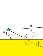
Figure 12: Relationship between the positions of the source, the detector and the notional “image” detector.

As $R$ tends to a value much larger than $c/\omega$ along this narrow beam, the nonspherically-decaying component of the radiation dominates over the conventional component. At shorter distances from the source, however, the detected power receives contributions from both of these components. If the fitting includes data for relatively small values of $R$ (see e.g. the solid curves in Figs. 10(b) and (c)), both spherically- and non-spherically-decaying contributions must be combined as follows:

$${\cal P}_{\parallel,\perp}\propto\Big{|}{\exp[{\rm i}(kR+\pi/4)]\over R^{\kappa}}+K{\exp({\rm i}kR)\over R}+Q_{\parallel,\perp}\Big{[}{\exp[{\rm i}(kR_{\rm r}+\pi/4)]\over R_{\rm r}^{\kappa}}+K{\exp[{\rm i}(kR_{\rm r})]\over R_{\rm r}}\Big{]}\Big{|}^{2}.$$ (19)

Here, the constant $K$ stands for the relative strengths of the sources of the two components, and $\pi/4$ is the phase difference betweem them (see [12, 13]).

Extension to a volume source: description of the direct and reflected rays in terms of the experimentally measured coordinates

The modeling of the data is based on the same coordinates as those used in the theory papers [12, 13], shown in Fig. 3(c,d). In these coordinates, the source consists of the arc $-\pi/36<\varphi<\pi/36$ of a circular strip, centered on the origin, with the radius $a=10.025$ m and the thickness $\Delta r=0.05$ m. The source velocity points in the direction of increasing $\varphi$ (see Fig. 3(d); its angular velocity points in the direction of positive $z$). Since the position of the source in Fig. 3(a) is such that its velocity points from the left to the right, the spherical coordinates $(R_{P},\theta_{P},\varphi_{P})$ of Refs. [12, 13] have to be based, in the present case, on a Cartesian system whose $z$-axis points downward, as in Fig. 3(c). (The midpoint of the source arc lies on the $x$-axis of this underlying Cartesian system; see Fig. 3(c).)

For comparing the data with the theoretical predictions, we need to express $(R_{\rm P},\theta_{\rm P},\varphi_{\rm P})$ in terms of the experimentally measured coordinates $(R,\vartheta_{\rm V},\phi_{\rm V})$ and $(R,\vartheta_{\rm H},\phi_{\rm H})$ of Figs. 3(a) and 3(b).

The Cartesian system $(x^{\prime},y^{\prime},z^{\prime})$ corresponding to the spherical coordinates $(R,\vartheta_{V},\phi_{V})$ of Fig. 3(a) differs from the Cartesian system $(x,y,z)$ corresponding to the spherical coordinates $(R_{\rm P},\theta_{\rm P},\varphi_{\rm P})$ of Fig. 3(c) in that its origin is shifted by the array radius $a$ along the positive $x$-axis, its $x$ and $y$ axes are interchanged, and its $z$-axis is inverted:

$$x^{\prime}=y,\quad y^{\prime}=x-a,\quad z^{\prime}=-z.$$ (20)

The Cartesian and polar coordinates of the observation point P in the reference frame shown in Fig. 3(a) are related by

$$x^{\prime}=R\cos\vartheta_{\rm V}\cos\phi_{\rm V},\quad y^{\prime}=R\cos\vartheta_{\rm V}\sin\phi_{\rm V},\quad z^{\prime}=R\sin\vartheta.$$ (21)

These, together with the corresponding coordinates of P in the reference frame shown in Figs. 3(c), (d),

$$x=R_{\rm P}\sin\theta_{\rm P}\cos\varphi_{\rm P},\quad y=R_{\rm P}\sin\theta_{\rm P}\sin\varphi_{\rm P},\quad z=R\cos\theta_{\rm P},$$ (22)

yield the first required transformation:

$$R_{\rm P}=(R^{2}+a^{2}+2aR\cos\vartheta_{\rm V}\sin\phi_{\rm V})^{1/2},$$

$$\theta_{\rm P}=\arccos\Big{(}-{R\over R_{\rm P}}\sin\vartheta_{\rm V}\Big{)},$$

$$\varphi_{\rm P}=-3\pi/2-\arctan\Big{(}\tan\phi_{\rm V}+{a\over R\cos\vartheta_{\rm V}\cos\phi_{\rm V}}\Big{)}.$$ (23)

In Fig. 3(b), the position vector of the observation point P is projected onto the $(x^{\prime},z^{\prime})$ plane of the shifted Cartesian system $(x^{\prime},y^{\prime},z^{\prime})$, so that

$$x^{\prime}=R\cos\phi_{\rm H}\cos\vartheta_{\rm H},\quad y^{\prime}=R\sin\phi_{\rm H},\quad z^{\prime}=R\cos\phi_{\rm H}\sin\vartheta_{\rm H}.$$ (24)

Rewriting these expressions for $(x^{\prime},y^{\prime},z^{\prime})$ in terms of $(R_{\rm P},\theta_{\rm P},\varphi_{\rm P})$, via $(x,y,z)$, and solving for $R_{\rm P}$, $\theta_{\rm P}$ and $\varphi_{\rm P}$, we obtain the second required transformation:

$$R_{\rm P}=(R^{2}+a^{2}+2aR\sin\phi_{\rm H})^{1/2},$$

$$\theta_{\rm P}=\arccos\Big{(}-{R\over R_{\rm P}}\cos\phi_{\rm H}\sin\vartheta_{\rm H}\Big{)},$$

$$\varphi_{\rm P}=-3\pi/2-\arctan\Big{(}{\tan\phi_{\rm H}\over\cos\vartheta_{\rm H}}+{a\over R\cos\phi_{\rm H}\cos\vartheta_{\rm H}}\Big{)}.$$ (25)

Having expressed the position vector ${\bf x}_{\rm P}=(R_{\rm P},\theta_{\rm P},\varphi_{\rm P})$ of the detector in terms of the experimentally measured coordinates, we now know how to determine the characteristics of the direct ray ${\bf x}_{\rm P}-{\bf x}$ that links each source element ${\bf x}=(r,\varphi,z)$ of the array to the observation point P. The next step is to determine the corresponding characteristics of the reflected rays that reach P from various volume elements of the array. As we have already seen in the treatment of a simple dipole aerial, both the angle $\alpha$ that a given reflected ray makes with the normal to the ground, ${\hat{\bf e}}_{g}$, and the distance $R_{r}$ that this wave traverses to reach the detector at P (see Fig. 12) can be easily inferred from the position vector ${\bf x}_{\rm P^{\prime}}$ of the image P^′ of P with respect to the ground. We proceed to determine ${\bf x}_{\rm P^{\prime}}$ in terms both of the coordinates $(R,\vartheta_{V},\phi_{V})$ and of the coordinates $(R,\vartheta_{H},\phi_{H})$.

Suppose that the plane of the array is vertical, as in Fig. 3(a), and that the upward-pointing normal to the ground at the point of reflection, ${\hat{\bf e}}_{\rm g}$, makes the angle $\phi_{0}$ with the positive $x$-axis of the $(x,y,z)$ frame (whose $z$-axis is in this case parallel to the ground), i.e.

$${\hat{\bf e}}_{\rm g}=\cos\phi_{0}{\hat{\bf e}}_{x}-\sin\phi_{0}{\hat{\bf e}}_{y}.$$ (26)

(For a smooth and perfectly horizontal ground, $\phi_{0}$ is related to $\phi_{\rm V}$ via $\phi_{0}-\phi_{\rm V}=\arcsin[(h_{\rm A}-h_{\rm D})/R]$.) Then the position vector, in the $(x,y,z)$ frame, of the image P^′ of P across the earth’s surface can be written as

$${\bf x}_{\rm P^{\prime}}={\bf R}+a{\hat{\bf e}}_{x}-2h_{\rm D}{\hat{\bf e}}_{\rm g},$$ (27)

where ${\bf R}$ is the position vector of P in the $(x^{\prime},y^{\prime},z^{\prime})$ frame, the frame whose origin lies at the midpoint of the array (see Figs. 3(c) and 12).

The following expressions for ${\bf x}_{\rm P^{\prime}}$ and ${\bf R}$ in terms of their components in the $(x,y,z)$ and the $(x^{\prime},y^{\prime},z^{\prime})$ frames,

$${\bf x}_{\rm P^{\prime}}=R_{\rm P^{\prime}}\sin\theta_{\rm P^{\prime}}(\cos\varphi_{\rm P^{\prime}}{\hat{\bf e}}_{x}+\sin\varphi_{\rm P^{\prime}}{\hat{\bf e}}_{y})+R_{\rm P^{\prime}}\cos\theta_{\rm P^{\prime}}{\hat{\bf e}}_{z},$$ (28)

$${\bf R}=R\cos\vartheta_{\rm V}(\cos\phi_{\rm V}{\hat{\bf e}}_{x^{\prime}}+\sin\phi_{\rm V}{\hat{\bf e}}_{y^{\prime}})+R\sin\vartheta_{\rm V}{\hat{\bf e}}_{z^{\prime}},$$ (29)

together with the relationships

$${\hat{\bf e}}_{x^{\prime}}={\hat{\bf e}}_{y},\quad{\hat{\bf e}}_{y^{\prime}}={\hat{\bf e}}_{x},\quad{\hat{\bf e}}_{z^{\prime}}=-{\hat{\bf e}}_{z}$$ (30)

between the base vectors of these two frames (see Eq. 20) therefore yield

$$R_{\rm P^{\prime}}=[R^{2}+a^{2}+(2h_{\rm D})^{2}-4ah_{\rm D}\cos\phi_{0}+2aR\cos\vartheta_{\rm V}\sin\phi_{\rm V}-4h_{\rm D}R\cos\vartheta_{\rm V}\sin(\phi_{\rm V}-\phi_{0})]^{1/2},$$

$$\theta_{\rm P^{\prime}}=\arccos\Big{(}-{R\over R_{\rm P^{\prime}}}\sin\vartheta_{\rm V}\Big{)},$$

$$\varphi_{\rm P^{\prime}}=-3\pi/2-\arctan\Big{(}{{R\cos\vartheta_{\rm V}\sin\phi_{\rm V}+a-2h_{\rm D}\cos\phi_{0}}\over{R\cos\vartheta_{\rm V}\cos\phi_{\rm V}+2h_{\rm D}\sin\phi_{0}}}\Big{)},$$ (31)

for the spherical coordinates of the image point P^′ in terms of the angles $(\vartheta_{\rm V},\phi_{\rm V})$ of Fig. 3(a).

To determine ${\bf x}_{\rm P^{\prime}}$ in terms of the coordinates $(R,\vartheta_{H},\phi_{H})$ of Fig. 3(b), suppose that the upward-pointing normal to the ground, at the point of reflection, makes the angle $\vartheta_{0}$ with the negative $z$-axis of the $(x,y,z)$ frame (whose $x$-axis is in this case parallel to the ground), i.e.

$${\hat{\bf e}}_{\rm g}=-\sin\vartheta_{0}{\hat{\bf e}}_{y}-\cos\vartheta_{0}{\hat{\bf e}}_{z}.$$ (32)

(Here, too, $\vartheta_{0}$ is related to $\vartheta_{\rm H}$ via $\vartheta_{0}-\vartheta_{\rm H}=\arcsin[(h_{\rm A}-h_{\rm D})]/R$ when the ground is smooth and horizontal.)

Inserting this alternative expression for ${\hat{\bf e}}_{\rm g}$ in Eq. 27 and using Eqs. 28, 30, and the following version of Eq. 24,

$${\bf R}=R\cos\phi_{\rm H}(\cos\vartheta_{\rm H}{\hat{\bf e}}_{x^{\prime}}+\sin\vartheta_{\rm H}{\hat{\bf e}}_{z^{\prime}})+R\sin\phi_{\rm H}{\hat{\bf e}}_{y^{\prime}},$$ (33)

we obtain

$$R_{\rm P^{\prime}}=[R^{2}+a^{2}+(2h_{\rm D})^{2}+2aR\sin\phi_{\rm H}-4h_{\rm D}R\cos\phi_{\rm H}\sin(\vartheta_{\rm H}-\vartheta_{0})]^{1/2},$$

$$\theta_{\rm P^{\prime}}=\arccos\Big{(}-{{R\cos\phi_{\rm H}\sin\vartheta_{\rm H}-2h_{\rm D}\cos\vartheta_{0}}\over R_{\rm P^{\prime}}}\Big{)},$$

$$\varphi_{\rm P^{\prime}}=-3\pi/2-\arctan\Big{(}{{R\sin\phi_{\rm H}+a}\over{R\cos\phi_{\rm H}\cos\vartheta_{\rm H}+2h_{\rm D}\sin\vartheta_{0}}}\Big{)},$$ (34)

for the spherical coordinates of the image point P^′, with respect to the $(x,y,z)$ frame in terms of the angles $(\vartheta_{H},\phi_{H})$ of Fig. 3(b).

Theoretical treatment of the spherically-decaying component of the emission from the experimental array

We now describe the use of the theory of Refs. [12, 13] to model the emissions of the experimental array. Our purpose is to predict the beaming of the spherically-decaying component of the radiation; relevant data are shown in Figs. 5-9. (The detailed behavior of the nonspherically-decaying component will be left for a future work.) The same mathematical notation as that in Refs. [12, 13] is used; for consistency with the original papers, we employ Gaussian electromagnetic units.

We commence with the following far-field expressions for the electromagnetic fields E and B in the absence of boundaries [Eqn. (14) of Ref. [12]]:

$${\bf E}\simeq{1\over c^{2}}\int{\rm d}^{3}x\,{\rm d}t\,{\delta(t_{\rm P}-t-|{\bf x}_{\rm P}-{\bf x}|/c)\over|{\bf x}_{\rm P}-{\bf x}|}{\hat{\bf n}}{\bf\times}\Big{(}{\hat{\bf n}}{\bf\times}{\partial{\bf j}\over\partial t}\Big{)}~{}~{}~{}{\rm;}~{}~{}~{}{\bf B}={\hat{\bf n}}\times{\bf E}.$$ (35)

Here $t_{\rm P}$ is the time at which the field is measured at the observation point P, and ${\bf x}$ and $t$ are the position of a source element and the retarded time, respectively; ${\hat{\bf n}}={\bf x}_{\rm P}/|{\bf x}_{\rm P}|$ is a unit vector along the direction linking the source that is localized in the vicinity of the origin and the observer at P. For the polarization ${\bf P}$ described in Eq. 2, whose distribution pattern both rotates (with an angular frequency $\omega$) and oscillates (with a frequency $\Omega$), the source term in the above expression is related to the cylindrical components $(s_{r},s_{\varphi},s_{z})$ of the vector ${\bf s}$ that designates the direction of the current density ${\bf j}=\partial{\bf P}/\partial t$ by

$${\hat{\bf n}}{\bf\times}({\hat{\bf n}}{\bf\times}\partial{\bf j}/\partial t)=\textstyle{1\over 4}\omega^{2} \sum_{\mu=\mu_{\pm}}\mu^{2}\exp[-{\rm i}(\mu{\hat{\varphi}}-\Omega\varphi/\omega)]\big{\{}[s_{\varphi}\cos\theta_{P}\sin(\varphi-\varphi_{P})$$ (36)

$$-s_{r}\cos\theta_{P}\cos(\varphi-\varphi_{P})+s_{z}\sin\theta_{P}]{\hat{\bf e}}_{\perp}+[s_{r}\sin(\varphi-\varphi_{P})$$ (37)

$$+s_{\varphi}\cos(\varphi-\varphi_{P})]{\hat{\bf e}}_{\parallel}\big{\}}+\{m\to-m,\Omega\to-\Omega\},\qquad$$ (38)

where the cylindrical coordinates $(r,\varphi,z)$ and $(r_{\rm P},\varphi_{\rm P},z_{\rm P})$ of ${\bf x}$ and ${\bf x}_{\rm P}$ are with respect to the $(x,y,z)$ frame shown in Fig. 3(c), ${\hat{\varphi}}\equiv\varphi-\omega t$, $\mu_{\pm}\equiv(\Omega/\omega)\pm m$, ${\hat{\bf e}}_{\parallel}={\hat{\bf e}}_{\varphi_{P}}$ (which is parallel to the plane of rotation) and ${\hat{\bf e}}_{\perp}={\hat{\bf n}}\times{\hat{\bf e}}_{\parallel}$ are a pair of unit vectors normal to the radiation direction ${\hat{\bf n}}$, and the symbol $\{m\to-m,\Omega\to-\Omega\}$ designates a term exactly like the one preceding it but in which $m$ and $\Omega$ are everywhere replaced by $-m$ and $-\Omega$, respectively. This is Eq. (18) of Ref. [12].

We are interested in the context of the present measurements in the radiation that is polarized parallel to the plane of the array; note also that the component $s_{\varphi}$ is zero in the experimental array described in the current paper. Hence, the relevant component of the source term in Eq. 38 is

$${\hat{\bf e}}_{\parallel}\cdot[{\hat{\bf n}}\times({\hat{\bf n}}\times\partial{\bf j}/\partial t)]=\textstyle{1\over 2}s_{r}\sin(\varphi-\varphi_{P})\Re\Big{\{}\sum_{\pm}(\Omega\pm m\omega)^{2}\exp\{{\rm i}[(\Omega\pm m\omega)t\mp m\varphi]\}\Big{\}},$$ (39)

where $\Re\{Z\}$ denotes the real part of $Z$. The fact that the array has the form of an arc means that the domain of integration in Eq. 35 consists, in the present case, of the cylindrical strip $-5^{\circ}<\varphi<5^{\circ}$, $10.00$ m$<r<10.05$ m, $-0.005$ m $<z<$ $0.005$ m, that bounds the volume occupied by the array (see Fig. 1). Since the $r$ and $z$ dimensions of this volume are appreciably shorter than the wavelengths at which the radiation is generated and measured in the present experiments ($0.50$ m and $0.59$ m), the integration with respect to these two coordinates may be omitted when evaluating the integral in Eq. 35 without introducing any significant error. (It must be emphasized that this approximation may only be used in the case of the spherically-decaying component of the emission; it is necessary to include the full volume of the source when calculating the nonspherically-decaying component. For the current purposes–modeling the spherically-decaying data of Figs. 5-9–the approximation is adequate.)

Inserting Eq. 39 in Eq. 35 and performing the trivial integration with respect to $t$, we find that the electric field of the radiation that is detected at either the frequency $f_{+}=\Omega+m\omega\equiv n_{+}\omega$ or the frequency $f_{-}=|\Omega-m\omega|\equiv|n_{-}|\omega$ (see Table 1 [12, 13]) is given by

$${\bf E}(f_{\pm})\propto\Re\Big{\{}\exp(-{\rm i}n_{\pm}\omega t_{\rm P})\int_{-\pi/36}^{\pi/36}d\varphi\,\sin(\varphi-\varphi_{\rm P})\exp[{\rm i}(n_{\pm}{\hat{R}}\pm m\varphi)]/{\hat{R}}\Big{\}}{\hat{\bf e}}_{\varphi_{\rm P}}$$ (40)

to within a constant of proportionality depending on the source strength. Here,

$${\hat{R}}\equiv|{\bf x}_{\rm P}-{\bf x}|\omega/c=[{{\hat{R}}_{\rm P}}^{2}+{\hat{r}}^{2}-2{\hat{r}}{\hat{R}}_{\rm P}\sin\theta_{P}\cos(\varphi-\varphi_{P})]^{1\over 2},$$ (41)

in which ${\hat{r}}\equiv r\omega/c$ is the source speed in units of $c$, ${\hat{R}}_{\rm P}\equiv R_{\rm P}\omega/c=({r_{\rm P}}^{2}+{z_{\rm P}}^{2})^{1\over 2}$, and $\theta_{\rm P}=\arccos(z_{\rm P}/R_{\rm P})$ [i.e. $({\hat{R}}_{\rm P},\theta_{\rm P},\varphi_{\rm P})$ comprise the spherical coordinates of P in units of the light-cylinder radius $c/\omega$].

The expression in Eq. 40 yields the electric-field vector of the wave that propagates from the source to the detector directly. The corresponding expression for the electric-field vector of the reflected wave is given by a similar expression in which the coordinates $(R_{\rm P},\theta_{\rm P},\varphi_{\rm P})$ of P are replaced by the coordinates $(R_{\rm r},\theta_{\rm P^{\prime}},\varphi_{\rm P^{\prime}})$ of the image P^′ of P and the integral is multiplied by one of the Fresnel coefficients $q_{\parallel}$ or $q_{\perp}$ (see the preceding subsections):

$${\bf E}_{\rm r}(f_{\pm})\propto\Re\Big{\{}q_{\parallel,\perp}\exp(-{\rm i}n_{\pm}\omega t_{\rm P})\int_{-\pi/36}^{\pi/36}d\varphi\,\sin(\varphi-\varphi_{\rm P^{\prime}})\exp[{\rm i}(n_{\pm}{\hat{R}_{\rm r}}\pm m\varphi)]/{\hat{R}_{\rm r}}\Big{\}}{\hat{\bf e}}_{\rm r},$$ (42)

where

$${\hat{R}}_{\rm r}\equiv[{{\hat{R}}_{\rm P^{\prime}}}^{2}+{\hat{r}}^{2}-2{\hat{r}}{\hat{R}}_{\rm P^{\prime}}\sin\theta_{\rm P^{\prime}}\cos(\varphi-\varphi_{\rm P^{\prime}})]^{1\over 2}.$$ (43)

The reflected radiation is polarized along

$${\hat{\bf e}}_{\rm rw}={\hat{\bf e}}_{\varphi_{\rm P}}$$ (44)

if ${\bf E}(f_{\pm})$ is normal to the plane of incidence, and along

$${\hat{\bf e}}_{\rm rw}=2({\hat{\bf e}}_{\rm g}\cdot{\hat{\bf e}}_{\varphi_{\rm P^{\prime}}}){\hat{\bf e}}_{\rm g}-{\hat{\bf e}}_{\varphi_{\rm P^{\prime}}}$$ (45)

if ${\bf E}(f_{\pm})$ is parallel to the plane of incidence, where ${\hat{\bf e}}_{g}$ is the upward-pointing unit vector perpendicular to the ground (see Eqs. 12 and 13). The coordinates $(R_{\rm P^{\prime}},\theta_{\rm P^{\prime}},\varphi_{\rm P^{\prime}})$ have the values derived in Eq. 31 when the array is positioned as in Fig. 3(a), and those derived in Eq. 34 when the array is positioned as in Fig. 3(b). The values of $q_{\parallel}$ and $q_{\perp}$ appear in Eqs. 14 and 15.

Next, we need to find the power that is received at P by an observer whose detector only picks up radiation of a given polarization, e.g. a polarization along the unit vector ${\hat{\bf p}}$. This can be done by adding the components ${\hat{\bf p}}\cdot{\bf E}(f_{\pm})$ and ${\hat{\bf p}}\cdot{{\bf E}_{\rm r}}(f_{\pm})$ of the electric-field vectors of the direct and the reflected waves and averaging the square of the resulting expression over the observation time $t_{\rm P}$. The result is

$${\cal P}_{\parallel,\perp}(f_{\pm})\propto\bigg{|} {\hat{\bf p}}\cdot{\hat{\bf e}}_{\varphi_{\rm P}}\int_{-\pi/36}^{\pi/36}d\varphi\,\sin(\varphi-\varphi_{\rm P})\exp[{\rm i}(n_{\pm}{\hat{R}}\pm m\varphi)]/{\hat{R}}$$ (46)

$$+q_{\parallel,\perp}{\hat{\bf p}}\cdot{\hat{\bf e}}_{\rm rw}\int_{-\pi/36}^{\pi/36}d\varphi\,\sin(\varphi-\varphi_{\rm P^{\prime}})\exp[{\rm i}(n_{\pm}{\hat{R}}_{\rm r}\pm m\varphi)]/{\hat{R}}_{\rm r}\bigg{|}^{2},$$ (47)

a general result that applies to both frequencies, irrespective of whether the radiation is polarized parallel or perpendicular to the plane of incidence.

When the array is positioned as in Fig. 3(b), the generated radiation is polarized horizontally, i.e. in a direction normal to the plane of incidence. In this case, ${\hat{\bf p}}\cdot{\hat{\bf e}}_{\varphi_{\rm P}}$ and ${\hat{\bf p}}\cdot{\hat{\bf e}}_{\rm rw}$ in the above equation are equal and so can be factored out and absorbed in the constant of proportionality. But when the plane of the array is vertical, as in Fig. 3(a), the electric-field vectors of the generated and reflected waves, though both in the plane of incidence, are no longer parallel to each other. In such experiments, we have used a receiving antenna whose polarization is vertical, i.e. for which ${\hat{\bf p}}={\hat{\bf e}}_{\rm g}$. According to Eqs. 26 and 45, therefore, the factors in question have the values ${\hat{\bf p}}\cdot{\hat{\bf e}}_{\varphi_{\rm P}}=-\sin(\varphi_{\rm P}+\phi_{0})$ and ${\hat{\bf p}}\cdot{\hat{\bf e}}_{\rm rw}=-\sin(\varphi_{\rm P^{\prime}}+\phi_{0})$ in these experiments.

Note that the emission is beamed when the phase of the rapidly oscillating exponential in the integrand of Eq. 40 has a stationary point within the domain of integration, i.e. when

$${\partial\over{\partial\varphi}}[n_{\pm}{\hat{R}}\pm m(\varphi-\varphi_{\rm P})]$$ (48)

vanishes for a value of $\varphi$ in $-\pi/36<\varphi<\pi/36$. This stationary point would be degenerate, and so the beaming would be tighter, if

$${\partial^{2}\over{\partial\varphi^{2}}}[n_{\pm}{\hat{R}}\pm m(\varphi-\varphi_{\rm P})]$$ (49)

vanishes at the same time. The above two conditions are satisfied simultaneously when

$${\hat{r}}=\frac{\omega r}{c}={m\over{|n_{\pm}|}}\Big{[}{{1-m^{2}/(n_{\pm}{\hat{R}}_{\rm P})^{2}}\over{\sin^{2}\theta_{\rm P}-m^{2}/(n_{\pm}{\hat{R}}_{\rm P})^{2}}}\Big{]}^{1\over 2},$$ (50)

and so the phase in question is stationary at $\varphi=\varphi_{\rm P}+2\pi-\arccos[m^{2}/({n_{\pm}}^{2}{\hat{r}}{\hat{r}}_{\rm P})]$ (cf. [12, 13]). The parameters in our experiments are chosen such that the value of $r$ implied by Eq. 50, for an observer in the far field, lies within the radial thickness $10.00$ m $<r<$ $10.05$ m of the array.

Adjustable parameters: effects of the array orientation and surface corrugations on the modeling of the beaming data

There are no truly adjustable parameters in the analysis of the beaming data (Figs. 5-9) in this paper, especially when $R~{}\mbox{{\raisebox{-1.72218pt}{$\stackrel{{\scriptstyle>}}{{{\scriptstyle\sim}}}$}}}~{}300$ m. The speed of the source is constrained by the setting of the experimental machine and the refractive index of the ground is determined by anciliary experiments with the dipole aerial (see Fig. 4). The measured heights $h_{\rm A}$ and $h_{\rm D}$ and distance $R$ are also used as input parameters. The remaining uncertainties come from the difficulties involved with modeling the reflection of curved wave fronts and small inaccuracies in the angular coordinates. We treat the latter first.

In modeling the experimental data of Figs. 5-9, variations in the parameters $\vartheta_{0}$ (see Eq. 32) and $\phi_{0}$ (see Eq. 26), the angles marking the orientation of the array, have a significant effect on the relative phases of the rays traveling on the direct and reflected paths (Fig. 12). Ideally, with flat ground (i.e. the runway) and precision measurements of the orientation of the array, these angles would be completely constrained by the measured experimental coordinates $\phi_{\rm V}$ and $\vartheta_{\rm H}$ respectively, plus the known $h_{\rm A}$, $h_{\rm D}$ and $R$. However, there are two problems with this approach:

1. The measurement of the angular coordinate desribing the tilting of the array is subject to relatively large fractional errors, $\sim\pm 0.5^{\circ}$;

2. The runway surface used for the measurement has distinct corrugations corresponding to fractions of a degree; over long distances, these can result in non-negligible shifts in the apparent position of the reflected ray.

These uncertainties were encompassed by making $\vartheta_{0}$ or $\phi_{0}$ (as appropriate) somewhat adjustable; adjustments of less than $\sim 1^{\circ}$ from the expected value (i.e. of the order of the uncertainty in the experimental angles) were in general sufficient to obtain very close agreement between model and data.

A second cause of uncertainty is the use of Fresnel coefficients in dealing with reflection from the ground; Fresnel coefficients are of course derived for plane wave fronts [15]. As is well known in the modeling of radar beams [17], wave fronts close to a source have significant curvature, leading to an apparent loss of the reflected radiation due to “phase smearing”. In the present case, the effect becomes noticeable for $R~{}\mbox{{\raisebox{-1.72218pt}{$\stackrel{{\scriptstyle<}}{{{\scriptstyle\sim}}}$}}}~{}300$ m.

A detailed treatment of curved wave fronts is very complex, and beyond the scope of this paper. However, a number of empirical approximations may be used [17]. Following these precedents, the reflection coefficient in simulations of the beaming involving distances $R~{}\mbox{{\raisebox{-1.72218pt}{$\stackrel{{\scriptstyle<}}{{{\scriptstyle\sim}}}$}}}~{}300$ m was scaled by a factor $q_{0}$, representing the loss of signal on reflection due to the curved wave fronts.

References

- [1] A. Sommerfeld, “Zur Elektronentheorie (3 Teile),” Nachrichten der Kgl. Gesellschaft der Wissenschaften zu Göttingen, math.-naturwiss. Klasse, 99–130, 363–439 (1904); 201–235 (1905).
- [2] For a historical survey, see chapters and papers by A. Einstein in “The Principle of Relativity”, eds W. Perrett and G.B. Jeffery (Dover, New York, 1958).
- [3] B. M. Bolotovskii and V. L. Ginzburg, “The Vavilov-Cerenkov effect and the Doppler effect in the motion of sources with superluminal velocity in vacuum,” Sov. Phys. Usp. 15, 184–192 (1972).
- [4] V. L. Ginzburg, Theoretical Physics and Astrophysics, Ch. VIII (Pergamon Press, Oxford, 1979).
- [5] B. M. Bolotovskii and V. P. Bykov, “Radiation by charges moving faster than light,” Sov. Phys. Usp. 33, 477–487 (1990).
- [6] H. Ardavan, “Generation of focused, nonspherically decaying pulses of electromagnetic radiation,” Phys. Rev. E 58, 6659–6684 (1998).
- [7] A. Hewish, “Comment I on ‘Generation of focused, nonspherically decaying pulses of electromagnetic radiation’,” Phys. Rev. E 62, 3007 (2000).
- [8] J. H. Hannay, “Comment II on ‘Generation of focused, nonspherically decaying pulses of electromagnetic radiation’,” Phys. Rev. E 62, 3008–3009 (2000).
- [9] H. Ardavan, “Reply to Comments on ‘Generation of focused, nonspherically decaying pulses of electromagnetic radiation’,” Phys. Rev. E 62, 3010–3013 (2000).
- [10] H. Ardavan, “The superluminal model of pulsars,” in “Pulsar Astronomy–2000 and Beyond (IAU Colloq. 177),” eds. M. Kramer, N. Wex, and R. Wielebinski (ASP Conf. Ser. 202, San Francisco, 2000), pp. 365–366.
- [11] M.V. Lowson, “Focusing of helicopter BVI noise”, J. Sound and Vibration, 190, 477–494 (1996).
- [12] H. Ardavan, A. Ardavan and J. Singleton, “Frequency spectrum of focused broadband pulses of electromagnetic radiation generated by polarization currents with superluminally rotating distribution patterns”, J. Opt. Soc. Am. A 20, 2137–2155 (2003).
- [13] H. Ardavan, A.Ardavan, and J. Singleton, “The spectral and polarization characteristics of the nonspherically decaying radiation generated by polarization currents with superluminally rotating distribution patterns”, J. Opt. Soc. Am. A 21, 858–872 (2004).
- [14] See, for example, “Aspects relative to the terrestrial broadcasting and mobile services”, Report 239-7 “Propagation statistics required for broadcasting services using the frequency range 30 to 1000 MHz”and Report 229-6 “Electrical characteristics of the surface of the Earth”, prepared by study groups of the International Telecommunication Union (ITU) (ITU, Geneva, 1990).
- [15] B.I. Bleaney and B. Bleaney, “Electricity and Magnetism”, (Oxford University Press, Third Edition, Oxford, 1976).
- [16] L.D. Landau and E.M. Lifshitz, “Electrodynamics of Continuous Media” (Pergamon Press, Oxford, 1975).
- [17] J.A. Stratton,“Electromagnetic Theory” (McGraw-Hill, New York, 1941), pp. 490–587.
- [18] See e.g. P. Duke, “Synchrotron Radiation— Production and Properties” (Oxford University Press, Oxford, 2000).
- [19] R. J. Mailloux, “Phased Array Antenna Handbook”, (Artech House, New York, 1993).
- [20] Salt marsh (i.e. very flat marshland soaked twice daily by the sea), level grass, a level gravel road and an airfield runway were used in these tests.
- [21] J.J. Egli, “Radio propagation above 40 Mc over irregular terrain”, Proc. IRE, October 1957, 1383–1391.
- [22] Y. Okumura, E. Ohmori and K. Fukuda, “Field strength and its variability in VHF and UHF land mobile service”, Rev. of the Electrical Communications Laboratory, 16, no. 9–10, 825–873 (1968).
- [23] Note that Eq. 2 is the same as Eq. 7 of Ref. [12] and Eq. 9a of Ref. [13].
- [24] J.C. Dainty, “Laser speckle and related phenomena” (Topics in Applied Physics Vol. 9, Springer, Berlin, 1975), Chapters 1–3.
- [25] J.A.N. Noronha, T. Bielawa, C.R. Anderson, D.G. Sweeney, S. Licul and W.A. Davis, “Designing Antennas for UWB Systems”, Microwaves and RF, June 2003, pp53-61.
- [26] A. Ardavan and H. Ardavan, “Apparatus for generating focused electromagnetic radiation,” International Patent Application, PCT–GB99–02943 (6 Sept. 1999).