Fast convergence of white noise cross-correlation measurement archived by vector average in both frequency and time domain

Abstract

White noise measurement can provide very useful information in addition to normal transport measurements. For example thermal noise measurement can be used at sub Kelvin temperature to determine the absolute electron temperature without applying any heating current. And shot noise measurements helped to understand the properties of nano and mesoscopic normal metal/superconductor structures. But at low temperature and for relatively small resistance it is difficult to measure the sample’s noise magnitude because the background thermal noise can be much larger and usually there are other pick-up noises. Cross correlation technique is one way to solve this problem. This article describes an improved cross correlation algorithm that averages in both frequency and time domain, and the realization of a simple instrument set-up with PC and sound card. With this set-up it is shown even with much larger background noise and pickup noises, 100pV/$\sqrt{Hz}$ white noise level can be easily measured in seconds. Compared to the normally used cross-correlation methods, it is several orders of magnitude faster.

I Introduction

Recently a lot of attention has been paid on the properties of S/N/S and N/N/N microbridge structures, and noise measurement (shot noise Kum96 ; Reu03 as well as thermal noise Hen99 ) was used as an additional technique besides transport measurements. But to measure the noise at cryogenic temperature is difficult since the sample noise usually is much smaller than the thermal noise of the components in the test circuit. Noise thermometry for electrons at low temperature was previously performed by current noise measurement with SQUID Rou85 , which is very sensitive and has very low noise level. However it is limited for small resistance and not for voltage noise measurement, also it can not be used when magnetic field is applied. Cross-correlation technique Sam99 ; Hen99 ; Kum96 provides an alternative method to measure the sample noise at low temperature. One bottleneck for this technique is that it requires a lot of time to do cross-correlation to converge and achieve the required sensitivity, and the trade off between sensitivity and the time needed to converge makes it difficult to use for low level noise experiments.

In this article we present an improved cross-correlation algorithm as well as the test instrument set-up for measurement of thermal noise. This algorithm does a vector average over both time and specific frequency range. It is worth noting that for commercial spectrum analyzer usually only average over time is used, and it is impossible to realize this algorithm within the instrument because of limitations like memory and computation speed. As shown in the following sections, much faster convergence can be achieved with the new algorithm.

II Cross correlation principle

It is well known 4-probe resistance measurement eliminates contact resistance by measuring the voltage signal across the sample that was stimulated by the current though the sample. It can be also considered as measuring the ”in phase” signal between current and voltage across the sample. Cross-correlation is similar in a sense it eliminates the channel’s noise by measuring the ”similarity” or ”in phase” signal between two different voltage channels. To better illustrate it, let consider the voltage signals from two channels. The Fourier components at particular frequency $\omega$ are:

$$\vec{v_{1}} = Ae^{i\theta_{A}}+N_{1}e^{i\theta_{1}}$$ (1)

$$\vec{v_{2}} = Ae^{i\theta_{A}}+N_{2}e^{i\theta_{2}}$$ (2)

Here A is the amplitude of the noise signal from our sample at frequency $\omega$ and $N_{1}$, $N_{2}$ are the amplitude of unwanted noise at $\omega$ generated in those two channels, for example, the thermal noise generated by the 20$\Omega$ lead resistor as shown in Fig. 1.

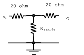
Figure 1: Schematic of the set-up. The sample resistor is 10 $\Omega$ and 1.5$\Omega$. The thermal noise is 20 $\Omega$ resistor along the channel is much bigger than the sample thermal noise.

To do cross-correlation we calculate the product of the two vectors:

$$\vec{v} = \vec{v_{1}}\cdot\vec{v_{2}}$$ (3)

$$= A^{2}+N_{1}N_{2}e^{i(\theta_{2}-\theta_{1})}+AN_{1}e^{i(\theta_{A}-\theta_{1})}+AN_{2}e^{i(\theta_{2}-\theta_{A})}$$

For the last three terms in Eq.3, since all those phases $\theta_{1}$, $\theta_{2}$ are random for white noise, and $A,N_{1}$ and $N_{2}$ does not change over time, when we do the average of $\vec{v}$ over enough long time, the random phase terms will cancel each other and will give negligible contribution to the total amplitude. So the real part of the $\vec{v}$ will converge at $A^{2}$, and the imaginary part will converge at $0$. Ideally if we do the average over infinite time the amplitude will converge at $A^{2}$. But in practical situation, the measurement time should be limited to some reasonable extent.

To estimate the time needed to approach convergence limit, we need to find when the deviation of the random phase term is much smaller than the $A^{2}$ term. First in order to identify the signals $\vec{v_{1}},\vec{v_{2}}$ at frequency $\omega$, the sampling time $\Delta T$ should be much longer than $1/\omega$ to get an accurate Fourier component. Then $\vec{v_{1}},\vec{v_{2}}$ at different times are acquired to do the vector average to eliminate the random phase terms. If $N_{1},N_{2}\gg A$, which happens when the sample is at low temperature and the sample signal amplitude $A$ is very small, it will take very long time to approach the convergence limit, which requires large n in the following equation:

$$N_{1}N_{2}\frac{\sum_{n}{e^{i(\theta_{2}-\theta_{1})}}}{n}\ll A^{2}$$

$$\overline{e^{i(\Delta\theta)}}=\frac{\sum_{n}{e^{i(\theta_{2}-\theta_{1})}}}{n}\ll 1$$ (4)

From standard textbookYat99 we know for iid (independent identical distributed) random sequence, n times average gives n times smaller variance. Assuming our channel noises are iid, we can expect that the variance of the averaged random phase term $Var(\overline{e^{i(\Delta\theta)}})\propto 1/n$, similarly for the averaged correlation the variance $Var(\overline{\vec{v}})\propto 1/n$, since our goal is to find noise magnitude $A$, we need the variance of root square of real part $\overline{\vec{v}}$, $Var(\sqrt{\overline{\Re{\vec{v}}}})$ which is proportional to $1/\sqrt{n}$, and finally what need standard deviation to compare with $A$. The standard deviation $\sigma_{\sqrt{\overline{\Re{\vec{v}}}}}=\sqrt{Var(\sqrt{\overline{\Re{\vec{v}}}})}$ should be proportional to $n^{-1/4}$. The $-1/4$ exponent is indeed observed in our experiment as shown in Sec.IV. This $-1/4$ exponent might also be used as a criteria to decide if the channel noise in different time steps can be fitted as iid random sequence, i.e. whether there is some correlation in time domain.

As indicated above by the $-1/4$ exponent, it is not very effective to eliminate the channel noise by increasing the measurement time steps. To accelerate the convergence process, a new algorithm is described below. Consider cross-correlation results at two different frequencies $\omega_{m}$ and $\omega_{n}$:

$$\vec{v_{m}} = A^{2}+N_{m}e^{i\theta_{m}}$$ (5)

$$\vec{v_{n}} = A^{2}+N_{n}e^{i\theta_{n}}$$ (6)

here the last vector term $N_{m}e^{i\theta_{m}}$ represents the vector sum of the last three terms in Eq.3. For ”white” noise, the amplitude $A$ is the same for different frequencies but the phases $\theta_{m}$, $\theta_{n}$ are random. This means a vector average over frequency domain is equivalent to the vector average over time domain. Since in practice we usually acquire a series of data points in one sampling time $\Delta T$ and then do a FFT transform, we could compute all the points in the frequency domain and use them to do vector average. For example the commercial spectrum analyzer usually takes 1024 scaler voltage points in $\Delta T$ (can’t take more because of limited memory) and give 512 vector points in the frequency domain. If we do vector average of the 512 points, according to the above statement it is similar to the result of average over 512 time steps for one particular frequency, which means the convergence at $A$ can be achieved 512 times faster. To test this we built some simple experimental set-up as described in the following section.

III Instrument set-up

A schematic plot of the test set up is shown in Fig. 1. Since people usually use resistive stainless steel coax cable to connect the sample in the low temperature stage, here a 20$\Omega$ resistor is used along each channel to simulate the channel resistor. The sample resistors used here are 10$\Omega$ and 1.5$\Omega$ to simulate the low noise level from real sample. In this case the amplitude of the sample noise $A$ is much smaller than that of channel noise $N$, so it can only be retrieved by cross-correlation technique.

The output of the two channels feeds separately to two PAR116 preamplifier (transformer mode) and PAR124 lock-in amplifier(only as an additional cascade amplifier, the Monitor output is used). The transformer is used to match the impedance. Two transformers need to be similar because otherwise if may change the phase and amplitude and affect the convergence. For example if there is a fixed phase difference $\Delta\theta$ between two transformer, the amplitude $A$ will be reduced to $cos(\Delta\theta)A$. After amplification the signals are fed to left/right channel input of a standard PCI sound card installed in a PII PC. The sound card then digitize the signal with 16 bit resolution and 44.1kHz sampling rates. After that the data is acquired by a program written in Labview to the computer memory. Then the program calculates Fourier spectra and and performs correlation and vector average etc., and shows all results on the screen in real time. A PC is much better than a commercial analyzer when considering the memory size and computation speed.

IV Experimental results

In Fig. 2, for the 10$\Omega$ sample resistor three curves are shown to demonstrate the result of conventional cross-correlation algorithm and to compare it with the new algorithm. Curve A shows that the standard deviation of the average over time, $\sigma_{\sqrt{\overline{\Re{\vec{v}}}}}$ decreases as the time elapsefootnote . As shown in Sec.II it is proportional to $n^{-1/4}$, which can be find easily from the log-log plot. Curve B shows the average over time approaches slowly to $A$, which is around 0.3nV/$\sqrt{Hz}$, after more than 100 times average. Curve C shows that when using the new algorithm, the average over frequency and time almost converge at $A$ from the first point! In fact, curve A is proportional to the difference between curve B and curve C. The measured amplitude of $A$ is close to expected amplitude of $A$, which is $\sqrt{4k_{B}TR}=$ 0.4nV/$\sqrt{Hz}$ for 10$\Omega$ sample resistor. This result is not bad when considering there may be affects from non ideal phase and amplitude properties of transformers and amplifiers, and uncertain pre-factors that came in from the data processing like the use of windows when doing FFT.

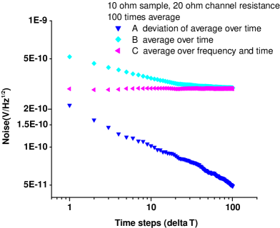
Figure 2: For a 10$\Omega$ sample resistor with 20$\Omega$ channel resistor, the cross-correlation results are shown. Curve A shows standard deviation of the average over time. The slope is proportional to $n^{-1/4}$. Curve B shows vector average over time. Curve C shows vector average over both frequency and time domain. With this new algorithm the convergence is achieved almost from the first point, much faster than the conventional cross-correlation result shown by curve B.

FFT spectrum after 100 times average is shown in Fig. 3. Curve B shows the result of the conventional cross-correlation vector average over 100 time steps. For comparison, curves C, D shows separately the noise spectrum of left/right channel measured in $\Delta T$. The vector average over both frequency and time domain is just a number, so it can not be shown in this frequency spectrum figure. From curve B, despite of those pick up noise peaks, we can still ”see” the real noise level that is around 0.3nV/$\sqrt{Hz}$, which was also found by the program and shown as the last point of curve B in Fig. 2. The program actually average scalarly the spectrum amplitude from 1kHz to 2kHz where the spectrum is almost flat and the affect of power line noise peaks is smaller. And those points close to power line noise peaks were abandoned. It is worth noting this scalarly average of amplitude over frequency is different with the vector average over frequency.

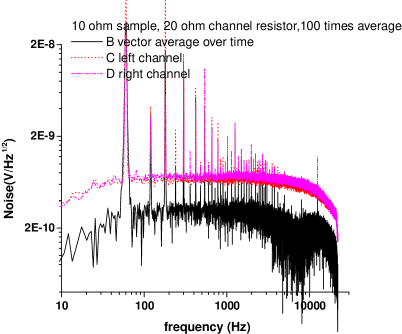
Figure 3: FFT spectrum after 100 times average. Curve B shows the cross-correlation vector average over 100 time steps, curve C, D shows the noise spectrum of left/right channel in $\Delta T$. The noise floor level of curve B is close to 0.3nV/$\sqrt{Hz}$ as shown in Fig. 2. The decrease of amplitude below 60Hz and the dip near 8kHz is due to the amplitude and phase properties of transformers. The cut-off near 22kHz is due to the Shannon limit, i.e., half of 44.1kHz sampling frequency.

With the presence of huge noise peaks as shown in Fig. 3, to observe the sample noise level it is required that the spectrum leakage and sidelobe background of the unwanted power line noise peaks shouldn’t mask the real white noise floor. This is usually achieved by using special window function when doing FFT and by increasing the frequency resolutionMan00 . Since Hann window has a fast decreasing sidelobe magnitude, it is preferred in this situation than uniform window which is conventionally used for flat noise spectrum measurement. And by increasing the frequency resolution the peaks’ mainlobe can be narrowed and their sidelobes can be attenuated. In our case the sampling rate is 44.1kHz, sampling number is chosen to be 32768 ($2^{15}$) points for each step, so the sampling time $\Delta T$ is $32768/44100=0.743$ second for each step, and frequency resolution $\Delta f$ is $1/0.743=1.346$Hz. It is possible to increase the sampling number to increase $\Delta T$ and decrease $\Delta f$. This will require only larger PC memory and higher speed CPU which is inexpensive. A simple algorithm is used here to eliminate 3 points from both sides of those power line peaks frequency when doing the average. This is already good enough to find the real noise floor of curve B in Fig. 3. More complex ways using adaptive filter program to remove the noise peak and extract the floor level is also possible.

As shown in Sec. II, the number of points used for vector average over frequency domain decides how much times faster of this new algorithm compared to conventional algorithm. Here since we used the range from 1kHz to 2kHz, with resolution 1.364Hz, we get 733 points. After subtracting the number of those points that are too close to noise peaks, we have around 600 points. So in principle we should get 600 times faster. To test this we measured room temperature noise for 1.5$\Omega$ sample resistor with same 20$\Omega$ channel resistors. The result is shown in Fig. 4. The start point of curve A and B are mostly determined by the 20$\Omega$ resistor. There is a ratio about 3 between those two curves around the start point. To detect the noise level from 1.5$\Omega$ sample resistor, we can assume the required standard deviation $\sigma$ to be 5 times smaller than the convergence limit $A$, which is $\sqrt{4k_{B}TR_{1.5\Omega}}$, we would need $\sigma$ decrease to magnitude $\sqrt{4k_{B}TR_{1.5\Omega}}/5$. The time needed for conventional cross-correlation methods can be estimated by:

$$(\frac{\sqrt{4k_{B}TR_{20\Omega}}/3}{\sqrt{4k_{B}TR_{1.5\Omega}}/5})^{4}\approx 1372$$ (7)

For the new algorithm, we expect $1372/600\approx 2$ steps.

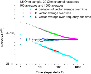
Figure 4: Two Cross-correlation test results for 1.5 $\Omega$ sample with 20$\Omega$ channel resistor, one stopped after 100 time steps, the other stopped after 1000 time steps. Curve B shows that using conventional average over time methods, it approaches convergence limit after 1000 averages. Curve C shows that using vector average over both frequency and time, the convergence was approached within a few time steps.

As shown in Fig. 4 the convergence limit is about 0.126 nV/$\sqrt{Hz}$. It is close to the estimated value of thermal noise level of a 1.5$\Omega$ resistor at room temperature, which is 0.158 nV/$\sqrt{Hz}$. And $0.126/0.158\approx 0.8$ is consistent with the 10$\Omega$ case. At 1000th time step, the last point of curve A in Fig. 4 has the value 25.6 pV/$\sqrt{Hz}$. The ratio between convergence limit and standard deviation is $126/25.6=4.9$, which is close to our estimation that is 5 for 1372 steps. As for curve C, it approaches the convergence limit from the first point in the 100 time step case, in the 1000 time steps case, despite of some fluctuations that may caused by some broad band noise or data processing, it also approaches the convergence limit from the first a few points. So it is proved that with the algorithm of vector average over frequency and time, convergence limit can be approached hundreds of times faster than conventional cross-correlation algorithm with this simple setup. If there are less noise peaks and if large frequency band is available, this algorithm could give even faster result.

V Conclusion

For white noise measurement, an improved cross-correlation algorithm using vector average over both frequency and time domain is presented. With consideration of low temperature noise measurement, a simple test set-up using PC and sound card is built and tested. It is proved that this algorithm can achieve convergence hundreds of times faster than the conventional cross-correlation algorithm. Even with much bigger channel noise and huge pick up noises, 100 pV/$\sqrt{Hz}$ noise level and 25pV/$\sqrt{Hz}$ sensitivity can be achieved in seconds. With a broader frequency band width, better A/D card and larger PC memory the convergence can be reached even faster. In principle this algorithm could be used for other type of noises as long as the shape of the spectrum is known and phase in frequency domain is random(for example 1/f noise).

References

- (1) M. Sampietro, L. Fasoli and G. Ferrari, Rev. Sci. Instrum. 70, 2520 (1999).
- (2) A. Kumar, L. Saminadayar, D. C. Glattli, Y. Jin and B. Etienne, Phys. Rev. Lett. 76, 2778 (1996).
- (3) M. Henny, S. Oberholzer, C. Strunk and C. Schonenberger, Phys. Rev. B 59, 2871 (1999).
- (4) M. L. Roukes, M. R. Freeman, R. S. Germain, R. C. Richardson and M. B. Ketchen, Phys. Rev. Lett. 55, 422 (1985).
- (5) Dimitris G. Manolakis, Vinay K. Ingle and Stephen M. Kogon, Statistical and adaptive signal processing : spectral estimation, signal modeling, adaptive filtering, and array processing(McGraw-Hill, Boston, 2000).
- (6) Roy D. Yates and David J. Goodman, Probability and stochastic processes : a friendly introduction for electrical andcomputer engineers(Wiley, New York, 1999).
- (7) B. Reulet, A. A. Kozhevnikov, D. E. Prober, W. Belzig and Yu. V. Nazarov, Phys. Rev. Lett. 90, 066601 (2003).
- (8) Curve A and B is smooth because in fact it is result of scalarly averaged of amplitude over a frequency range for every time step, and then vector average over time is conducted. This is further explained by Fig. 3.