The Brillouin Instability of intense laser in relativistic plasmas

Abstract

This paper studies the propagation of intense laser in plasmas in weak relativistic region($0.1<a_{0}^{2}<0.5$) using the quasi-periodic approximation. Effective Lorentz factor and density wave effects are calculated in detail. The relativistic correction on stimulated Brillouin instability is investigated in the rest parts. The coupled dispersion relations of Stimulated Brillouin Scattering(SBS) are obtained and investigated numerically.

1 Introduction

The propagation of intense laser through plasmas is an important concern in the laser-driven inertial confinement fusion, the laser-plasma accelerators, the x-ray laser and other physical problems [1]-[5]. In General, the amplitude of laser can be described by the normalized vector potential $\{\bf{a},\phi\}$, where $\mathbf{a}=\frac{e\mathbf{A}}{m_{0}c^{2}},\phi=\frac{e\Phi}{m_{0}c^{2}}$. While $a\ll 1$, the propagating equation of laser is linear. But many non-linear effects will appear when $a$ increases , such as density wave effects, relativistic mass correction, etc. While $a>1$, the problem becomes highly non-linear because of the relativistic effects and it can hardly be solved.

In full ionized plasmas, there are two dominating nonlinear effects on the laser propagation: one is the relativistic mass increase of the electron. When the amplitude of vector potential $a$ increases, the vibration velocity of electron increases and changes the mass of electron to $\gamma m$, where the Lorentz factor $\gamma=\frac{1}{\sqrt{1-v^{2}/c^{2}}}$ is a coefficient determined by the velocity, so non-linear effects appear.

The other important non-linear effect is the laser’s diffraction by electron density waves. When the intense laser propagates, electrons in the plasma first vibrate parallel to the electric field and perpendicular to the propagating direction of the laser. Then the vibrating elections are pushed by the Lorentz force produced by the magnet field of the laser. Electron density oscillations parallel to the propagating direction of the laser form density waves. Finally, laser is diffracted by the density waves. As is shown in the following, the density fluctuation is proportion to $\mathbf{a}\cdot\mathbf{a}$, its frequency is twice as the laser frequency and its order is the same as relativistic effect’s order. So the density wave must be considered in the relativistic region.

In the relativistic region, both non-linear effects cause corrections of the refract index of the plasma by modifying the dispersion relation of the laser. The correction is very important for the shaping and self-focusing of the intense laser pulse.

There are many parametric instabilities in plasmas such as Raman instability, Brillouin instability and $2\omega$ decay, etc. All these processes will be affected by the relativistic mass increase and the density wave effects. Stimulated Brillouin Scattering(SBS) is a very important phenomenon because it transfers almost all energy to the scattered light and reaches a maximum on backward scattering. In the case of backward SBS, it causes laser’s reflection and the energy loss. During the implosion of ICF, the Brillouin reflectivity can vary from 10%(for short wave incident laser) to more than 40% (for long wave laser)${}^{\cite[cite]{[\@@bibref{}{6}{}{}]}}$. In addition, the Brillouin Instability relates closely with the filamentation instability.

In recent papers[8][9], relativistic mass increase effects are investigated by introducing a Lorentz factor. However, because the Lorentz factor varies with the electron’s jitter velocity, it takes on different values for different non-linear effects and should be calculated separately in different cases. Besides, the SBS takes place in all the under-dense region of plasmas, while Stimulated Raman Scatter(SRS) can take place only in the low density region. Thus the density wave effects should be considered.

Some authors[10][11] already considered the density wave effects with the laser pulse propagation without handling the SBS instability. Besides, the density wave equation should be altered in the relativistic region (see sec. 2).

The purpose of this paper is to investigate the Brillouin instability of an intense laser with $a^{2}\sim 0.1-0.5$. We call this intensity region as Weak-Relativistic Region. Which indicates that the nonlinear effects can be processed by the series expansion with respect to $a^{2}$. For calculating the Brillouin effect ,we shall use the quasi-periodic approximation to handle density wave effects to get non-linear corrections of the laser’s dispersion relation with higher precision in sec. 2. In sec. 3, we shall investigate the Brillouin instability in the relativistic region.

2 The non-linear effects of the intense laser propagating in Plasmas

Consider the propagation of a linear-polarized laser in a cold plasma in which the electron’s thermal velocity is much smaller than their jitter speed in the laser field[12]. Suppose the laser is polarized in the $x$ direction and propagates in the $z$ direction with $a<1$. Assuming the plasma be homogeneous in the transverse direction, we have, from the conservation of transverse canonical momentum[2], $\gamma\beta_{x}=a_{x}$ and $\gamma\doteq\sqrt{1+\mathbf{a}^{2}}$, where $\bm{\beta}=\mathbf{v}/c$.

The laser propagation equation in this case has been derived by P. Sprangle and et al [13] as follows:

$$-\frac{\partial^{2}\mathbf{a}}{\partial c^{2}t^{2}}+\frac{\partial^{2}\bf{a}}{\partial z^{2}}=k_{p}^{2}\frac{n}{\gamma n_{0}}\mathbf{a}$$ (1)

where $n$ is the density of electrons, $n_{0}$ is the local average of $n$, $k_{p}=\omega_{p}/c$ and $\omega_{p}$ is the plasma frequency.

The plasma should satisfy Vlasov equation. In the cold plasma approximation we ignore the thermal-pressure to get the continuity equation and the equation of motion from the first two moments of the Vlasov equation:

$$\frac{\partial n}{\partial ct}\ +\frac{\partial(n\beta_{z})}{\partial z}=0$$ (2)

$$\frac{\partial(\gamma\beta_{z})}{\partial{ct}}+\beta_{z}\frac{\partial(\gamma\beta_{z})}{\partial z}=\frac{\partial\phi}{\partial z}-\frac{1}{2\gamma}\frac{\partial}{\partial z}{\mathbf{a}^{2}}$$ (3)

The above equations cannot be simplified to an ordinary wave equation as in non-relativistic case due to the presence of $\gamma$ under derivative operations. The non-linear effects must be treated separately for high frequency, low frequency and zero-frequency cases to get the correct dispersion relations.

In the quasi-periodic approximation we assume that the characteristic time of evolution of the laser pulse shape is much longer than the laser’s period, and $\mathbf{a}$ can be regarded approximately as a periodic function. Let $\mathbf{a}\doteq a_{0}\mathbf{\hat{x}}{\cos(\omega_{0}t-k_{0}z)}$, where $\mathbf{\hat{x}}$ is the unit vector in the $x$ direction. Now all of the coefficients and driving forces in eq. (2) and (3) are periodic functions, so its solutions should be periodic far from their instability region.

The approximation is similar to the quasi-stationary approximation used by P.Sprangle et al ${}^{\cite[cite]{[\@@bibref{}{13}{}{}]}}$, but now the phase velocity of the laser wave in the plasma, $\omega_{0}/k_{0}$, does not need be close to $c$. So this approximation can be used for dense plasmas.

Introduce the phase variable $\xi=\omega_{0}t-k_{0}z$ and let

$$n= n(\xi)$$

$$\beta_{z}= \beta_{z}(\xi)$$

$$\phi= \phi(\xi)$$

After simple calculations, (3)becomes

$$\frac{\omega_{0}^{2}}{k_{0}c^{2}}\frac{n_{0}}{n}\frac{d}{d\xi}({\gamma}\frac{n-n_{0}}{n})=\frac{\partial\phi}{\partial z}-\frac{1}{2\gamma}\frac{\partial}{\partial z}{\mathbf{a}^{2}}$$ (4)

Let $n=n_{0}(1+\psi)$ and use the poisson equation, the linearized equation in $\psi$ becomes

$$-\frac{\partial^{2}(\gamma\psi)}{\partial c^{2}t^{2}}=k_{p}^{2}\psi-\frac{\partial}{\partial z}(\frac{1}{2\gamma}\frac{\partial}{\partial z}(\mathbf{a}^{2}))$$ (5)

Expand the Lorentz factor $\gamma$ and preserve terms lower than fourth, we get the nonlinear dispersion relation by an iteration method:

$$\frac{\omega_{0}^{2}}{c^{2}}-k_{0}^{2}-k_{p}^{2}(1-\frac{3}{8}a_{0}^{2})=\frac{1}{2}k_{p}^{2}\psi_{0}=\frac{k_{p}^{2}}{2}\frac{k_{0}^{2}c^{2}a_{0}^{2}}{4\omega_{0}^{2}(1+\frac{1}{4}a_{0}^{2})-\omega_{p}^{2}}(1-\frac{1}{4}a_{0}^{2})$$ (6)

Here the relativistic terms appear with effective Lorentz factors $(1+\frac{1}{4}a_{0}^{2})$ and $(1+\frac{3}{8}a_{0}^{2})$ respectively. As we said before, the efficient Lorentz factors differ for different modes.The factor $\psi_{0}\propto k_{0}^{2}$ is the frequency-mixing term. The ratio $\psi_{0}/k_{0}^{2}$ increases while $\omega_{0}$ approaches $\omega_{p}$ . When $a_{0}^{2}\sim 0.3$ and $\omega_{0}^{2}=2\omega_{p}^{2}$,we have $\psi_{0}\sim 0.04$.

3 The relativistic correction of Stimulated Brillouin Instability

Consider a two-dimensional homogenous plasma and ignore the electron’s thermal motion in the direction of laser polarization. Let $\nabla_{\perp}=\{\frac{\partial}{\partial x},\frac{\partial}{\partial y}\}$, $\nabla^{2}_{\perp}=\frac{\partial^{2}}{\partial x^{2}}+\frac{\partial^{2}}{\partial y^{2}}$, $\bm{\beta}=\{v_{x}/c,v_{y}/c,v_{z}/c\}$, then $\nabla^{2}=\frac{\partial^{2}}{\partial z^{2}}+\nabla_{\perp}^{2}$.

Suppose that the incident laser propagates in $z$ direction and is polarized parallel to $x$ axis, the electron’s temperature in the plasma is $T$, then $kT\ll m_{0}v_{x}^{2}$. The conservation of the transverse canonical momentum leads to $\gamma v_{x}/c\approx a_{x}$. Now the Lorentz force has the following form $\mathbf{v}\times(\nabla\times\mathbf{a})\approx\frac{1}{2\gamma}\nabla(\mathbf{a}\cdot\mathbf{a})$,

So the equation of motion for electrons becomes

$$\frac{\partial}{\partial ct}(\gamma\bm{\beta})+(\bm{\beta}\cdot\nabla)(\gamma\bm{\beta})=\nabla\phi-\frac{1}{2\gamma}\nabla(\mathbf{a}\cdot\mathbf{a})-\nabla{\frac{P_{e}}{n_{0}m_{0}c^{2}}}$$ (7)

In stead of $P_{e}$, we shall introduce the normalized electron thermal-pressure $p=\frac{P_{e}}{m_{0}c^{2}}=\frac{(n_{0}+\tilde{n})\theta}{m_{0}c^{2}}$, where $\theta=kT$.

In Brillouin Scattering, the plasma acoustic wave is coupled with the laser wave. Let us consider low frequency fluctuations. Ignoring the electron’s inertia gives

$$\{\nabla\phi\}^{low}=\{\frac{1}{2\gamma}\nabla(\mathbf{a}^{2})\}^{low}-\frac{\theta}{m_{0}n_{0}c^{2}}\nabla(\tilde{n}^{low})$$

where $\{\}^{low}$ indicates preserving low frequency(acoustic) terms only.

Substituting this equation into ion’s equation of motion, ignoring ion’s thermal pressure($T_{i}\ll T_{e}$) and using the relation $Zn_{i}=n$ we have:

$$\frac{\partial^{2}\tilde{n}^{low}}{\partial c^{2}t^{2}}-\frac{Zn_{0}m_{0}}{M}\left\{[\nabla^{2}\sqrt{1+\mathbf{a}^{2}}]^{low}+\frac{\theta}{m_{0}c^{2}}\nabla^{2}(\frac{\tilde{n}^{low}}{n_{0}})\right\}=0$$

When $a<1$, $\sqrt{1+\mathbf{a}^{2}}\approx 1+\frac{1}{2}\mathbf{a}^{2}-\frac{1}{8}\mathbf{a}^{4}$. Let $\mathbf{a}=\mathbf{a_{L}}+\tilde{\mathbf{a}}_{s}$, where $\mathbf{a}_{L}$ and $\tilde{\mathbf{a}}_{s}$ is for the incident laser and the scattered light respectively.

Now use the relation $|\tilde{\mathbf{a}}_{s}|\ll|\mathbf{a}_{L}|$, we have

$$\frac{\partial^{2}\psi_{s}}{\partial t^{2}}-c_{s}^{2}\nabla^{2}\psi_{s}=\frac{Zm_{0}c^{2}}{M}\nabla^{2}(\mathbf{a}_{L}\cdot\tilde{\mathbf{a}}_{s}-\frac{1}{2}\mathbf{a_{L}}^{2}\mathbf{a}_{L}\cdot\tilde{\mathbf{a}_{s}})^{low}$$ (8)

where $\psi_{s}=\frac{\tilde{n}^{low}}{n_{0}}$ and $c_{s}=\sqrt{\frac{Z\theta}{M}}$ is the velocity of ion-acoustic wave in the plasma.

Similarly, we can write the density fluctuation in the form of $\psi=\frac{\tilde{n}}{n_{0}}=\psi_{L}+\tilde{\psi_{s}}$ and set up the modified propagation equation:

$$(-\frac{\partial^{2}}{\partial c^{2}t^{2}}+\frac{\partial^{2}}{\partial z^{2}}+\nabla_{\perp}^{2}-k_{p}^{2})\tilde{\mathbf{a}}_{s}=k_{p}^{2}[\psi_{L}\tilde{\mathbf{a}}_{s}+\tilde{\psi_{s}}\mathbf{a}_{L}]-\frac{3}{2}k_{p}^{2}\mathbf{a}_{L}^{2}\tilde{\mathbf{a}}_{s}$$ (9)

where $\psi_{L}$ is the density wave generated by the laser driving solely.

The coupled equations (8) and (9) are the fundamental equations for the Stimulated Brillouin Scattering in the weak relativistic region. There are two differences between the present equations and the normal Brillouin equations. First, the factor $\sqrt{1+\mathbf{a}^{2}}$ have replaced the factor $\frac{1}{2}\mathbf{a}^{2}$. Second, in the propagation equation, the density wave term $\psi_{L}\tilde{\mathbf{a}}_{s}$ and the relativistic term $\frac{3}{2}\mathbf{a}_{L}^{2}\tilde{\mathbf{a}}_{s}$ cause a new effect, which is the sideband mixing.

Assume that an acoustic density-perturbation is formed in the plasma: $n_{s}^{low}=n_{0}\psi_{a}\cos(\omega t-kz)$. It is coupled with the laser field in the plasma and produces the sideband scattered light waves like $\tilde{\mathbf{a}}_{s}=\mathbf{a}_{+}\cos[(\omega_{0}+\omega)t-(k_{0}+k)z]+\mathbf{a}_{-}\cos[(\omega_{0}-\omega)t-(k_{0}-k)z]$. In the linear region($a_{0}\ll 1$), the two scattered light waves will propagate independently and will not affect each other.

Let $\omega_{\pm}=\omega_{0}\pm\omega$, $k_{\pm}=k_{0}\pm k$, in the relativistic region we discussed, the laser will drive a density wave $\psi_{L}$ whose basic frequency is $2\omega_{0}$. This term will cause frequency mixing with $\mathbf{a}_{+}\cos(\omega_{+}t-k_{+}z)$ and result in a term whose frequency is $\omega_{-}$. Similarly, it will mix with $\mathbf{a}_{-}\cos(\omega_{-}t-k_{-}z)$ and result in a term with frequency $\omega_{+}$. Namely, two sideband light waves will be coupled to the basic mode. The term $\mathbf{a}_{L}^{2}$ in $\frac{3}{2}\mathbf{a}_{L}^{2}\tilde{\mathbf{a}}_{s}$ will act in the same way.

Because of the sideband mixing, $\mathbf{a}_{+}$ and $\mathbf{a}_{-}$ must be handled together to get cooperative dispersion relations of SBS.

We consider the simplest sideband mixing effects in order to get rid of the unnecessary complexity. Namely, we consider the mixing effects caused by $\psi_{L}\propto\cos(2\omega_{0}t-2k_{0}z)$ and $\mathbf{a_{L}^{2}}$ only. Assuming the incident laser propagates parallel to the $z$ axis and the scattered light propagate in the $y$-$z$ plane, the incident wave vector is $\{0,0,k_{0}\}$, the two scattered sideband wave vectors are $\{0,k_{\perp},k_{0}+k\}$ and $\{0,-k_{\perp},k_{0}-k\}$, we can write the incident laser in the form of $\mathbf{a}_{L}=a_{0}\hat{\mathbf{x}}\cos(\omega_{0}t-k_{0}z)$ , write the scattered light as $\tilde{\mathbf{a}_{s}}=\hat{\mathbf{x}}\{a_{+}\cos[(\omega_{0}+\omega)t-(k_{0}+k)z-k_{\perp}y]+a_{-}\cos[(\omega_{0}-\omega)t-(k_{0}-k)z+k_{\perp}y]\}$ and write the acoustic density fluctuation as $\tilde{\psi_{s}}=\psi_{a}\cos(\omega t-kz-k_{\perp}y)$. The sideband terms in the rhs of the propagation equation

$$(-\frac{\partial^{2}}{\partial c^{2}t^{2}}+\frac{\partial^{2}}{\partial z^{2}}+\nabla_{\perp}^{2}-k_{p}^{2})\tilde{\mathbf{a}}_{s}=k_{p}^{2}[\psi_{L}\tilde{\mathbf{a}}_{s}+\tilde{\psi_{s}}\mathbf{a}_{L}]-\frac{3}{2}k_{p}^{2}\mathbf{a}_{L}^{2}\tilde{\mathbf{a}}_{s}$$

are:

Sideband terms in $k_{p}^{2}\psi_{L}\tilde{\mathbf{a}_{s}}$ are

$$k_{p}^{2}\psi_{L}\tilde{\mathbf{a}_{s}}\longrightarrow\frac{1}{2}k_{p}^{2}\psi_{0}\{a_{-}\cos(\omega_{+}t-k_{+}z-k_{\perp}y)+a_{+}\cos(\omega_{-}t-k_{-}z+k_{\perp}y)\}$$

Sideband terms in $k_{p}^{2}\tilde{\psi_{s}}\mathbf{a}_{L}$ are

$$k_{p}^{2}\tilde{\psi_{s}}\mathbf{a}_{L}\longrightarrow\frac{k_{p}^{2}}{2}\psi_{a}a_{0}\{\cos(\omega_{+}t-k_{+}z-k_{\perp}y)+\cos(\omega_{-}t-k_{-}z+k_{\perp}y)\}$$

Finally, sideband terms in $-\frac{3}{2}k_{p}^{2}\mathbf{a}_{L}^{2}\tilde{\mathbf{a}_{s}}$ are

$$-\frac{3}{2}k_{p}^{2}\mathbf{a}_{L}^{2}\tilde{\mathbf{a}_{s}}\longrightarrow-\frac{3}{4}k_{p}^{2}a_{0}^{2}[a_{+}\cos(\omega_{+}t-k_{+}z-k_{\perp}y)+a_{-}\cos(\omega_{-}t-k_{-}z+k_{\perp}y)]$$

$$-\frac{3}{8}k_{p}^{2}a_{0}^{2}a_{+}\cos(\omega_{-}t-k_{-}z+k_{\perp}y)-\frac{3}{8}k_{p}^{2}a_{0}^{2}a_{-}\cos(\omega_{+}t-k_{+}z-k_{\perp}y)$$

Matching all the sideband terms, we get:

$$\bigg{\{}\begin{array}[]{cc}D_{+}a_{+}=\frac{1}{2}k_{p}^{2}\psi_{0}a_{-}+\frac{1}{2}k_{p}^{2}\psi_{a}a_{0}-\frac{3}{4}k_{p}^{2}a_{0}^{2}a_{+}-\frac{3}{8}k_{p}^{2}a_{0}^{2}a_{-}\\ D_{-}a_{-}=\frac{1}{2}k_{p}^{2}\psi_{0}a_{+}+\frac{1}{2}k_{p}^{2}\psi_{a}a_{0}-\frac{3}{4}k_{p}^{2}a_{0}^{2}a_{-}-\frac{3}{8}k_{p}^{2}a_{0}^{2}a_{+}\end{array}$$ (12)

where $D_{\pm}=\frac{\omega_{\pm}^{2}}{c^{2}}-k_{\pm}^{2}-k_{\perp}^{2}-k_{p}^{2}$.

$a_{+}$ and $a_{-}$ can be solved as

$$\Bigg{\{}\begin{array}[]{ccc}a_{+}=\frac{(D_{-}+\frac{3}{4}k_{p}^{2}a_{0}^{2})+(\frac{1}{2}k_{p}^{2}\psi_{0}-\frac{3}{8}k_{p}^{2}a_{0}^{2})}{(D_{+}+\frac{3}{4}k_{p}^{2}a_{0}^{2})(D_{-}+\frac{3}{4}k_{p}^{2}a_{0}^{2})-(\frac{1}{2}k_{p}^{2}\psi_{0}-\frac{3}{8}k_{p}^{2}a_{0}^{2})^{2}}\frac{1}{2}k_{p}^{2}\psi_{a}a_{0}\\ a_{-}=\frac{(D_{+}+\frac{3}{4}k_{p}^{2}a_{0}^{2})+(\frac{1}{2}k_{p}^{2}\psi_{0}-\frac{3}{8}k_{p}^{2}a_{0}^{2})}{(D_{+}+\frac{3}{4}k_{p}^{2}a_{0}^{2})(D_{-}+\frac{3}{4}k_{p}^{2}a_{0}^{2})-(\frac{1}{2}k_{p}^{2}\psi_{0}-\frac{3}{8}k_{p}^{2}a_{0}^{2})^{2}}\frac{1}{2}k_{p}^{2}\psi_{a}a_{0}\end{array}$$

The driving density wave equation is

$$\frac{\partial^{2}\tilde{\psi_{s}}}{\partial t^{2}}-c_{s}^{2}\nabla^{2}\tilde{\psi_{s}}=\frac{Zm_{0}c^{2}}{M}\nabla^{2}\left(\mathbf{a}_{L}\cdot\tilde{\mathbf{a}_{s}}-\frac{1}{2}\mathbf{a}_{L}^{2}\mathbf{a}_{L}\cdot\tilde{\mathbf{a}_{s}}\right)^{low}$$

$$=-\frac{Zm_{0}c^{2}}{M}\frac{1}{2}a_{0}(a_{+}+a_{-})(1-\frac{3}{8}a_{0}^{2})(k^{2}+k_{\perp}^{2})\cos(\omega t-kz-k_{\perp}y)$$ (14)

Substituting the above expression for $a_{\pm}$ into it, we get the Stimulated Brillouin Scattering’s dispersion relation:

$$\omega^{2}-c_{s}^{2}(k^{2}+k_{\perp}^{2})=\frac{Zm_{0}c^{2}}{M}\frac{1}{4}k_{p}^{2}(k^{2}+k_{\perp}^{2})(1-\frac{3}{8}a_{0}^{2})a_{0}^{2}$$

$$\times\frac{(D_{+}+D_{-})+k_{p}^{2}(\psi_{0}+\frac{3}{4}a_{0}^{2})}{(D_{+}+\frac{3}{4}k_{p}^{2}a_{0}^{2})(D_{-}+\frac{3}{4}k_{p}^{2}a_{0}^{2})-[\frac{1}{2}k_{p}^{2}(\psi_{0}-\frac{3}{4}a_{0}^{2})]^{2}}$$ (15)

This equation can be solved numerically. Let us consider the backward Brillouin scatter[1], when $k\simeq 2k_{0}$ and $k_{\perp}=0$. Let $\omega=\Omega\kappa_{p}c$,$k=\kappa k_{p}$,and $\Omega_{0}=\omega_{0}/{\omega_{p}}$, $\kappa_{0}=k_{0}/{k_{p}}$ ,we normalize the equation $(\ref{bri_dispersion})$ to

$$(\Omega^{2}-\kappa^{2}) =\frac{Zm_{0}}{M}\frac{1}{2}\kappa^{2}(1-\frac{3}{8}a_{0}^{2})a_{0}^{2}$$ (16)

$$\times\frac{\Omega^{2}\frac{c_{s}^{2}}{c^{2}}-\kappa^{2}+\psi_{0}}{[\Omega^{2}\frac{c_{s}^{2}}{c^{2}}-\kappa^{2}+\frac{1}{2}(\psi_{0}+\frac{3}{4}a_{0}^{2})]^{2}-4[\Omega\Omega_{0}\frac{c_{s}^{2}}{c^{2}}-\kappa\kappa_{0}]-\frac{1}{4}(\psi_{0}-\frac{3}{4}a_{0}^{2})^{2}}$$

We adopt the typical parameters $\frac{c_{s}}{c}=10^{-3}$,$\frac{M}{m}=1800$ ,the intensity of laser is set to $a_{0}^{2}=0.32$ ,the plasma density is set to $\omega_{0}^{2}=4\omega_{p}^{2}$ and $\omega_{0}^{2}=2\omega_{p}^{2}$ respectively. The results are plotted on figure 1 and figure 2. In the weak relativistic region,the ion acoustic waves become the quasi-mode whose frequency is determined by the laser intensity. Correspondingly, the relative value of growing rate and the laser frequency will far exceed the ratio $c_{s}/c$ and approach to $\frac{1}{40}$ in the region of the parameter we selected. It means that the Brillouin instability will have developed during about several tens to a few hundreds periods of the pump laser(about $10^{-13}-10^{-14}$ seconds ).

In the region we analyzed,the pure growing modes with $Re(\omega)=0$ appear at large $k$. First, The peak value of the growing rate locates near $k=2k_{p}$ and has a departure due to the relativistic effects. Then, the pure growing modes appear at large $k$ when the laser intensity and the plasma density increase. In the weak relativistic region, the pure growing modes form a plateau region. The pure growing mode at large $k$ will affect on some nonlinear effects like turbulence developing.

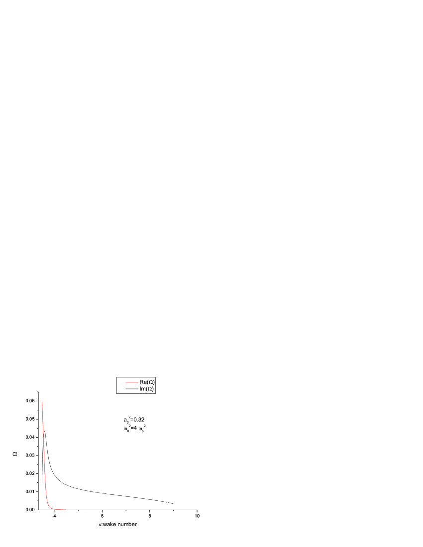
Figure 1: the growing rate when $n=\frac{1}{4}n_{0}$

.

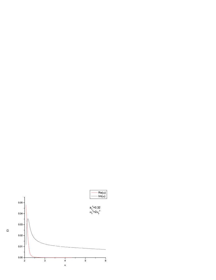
Figure 2: the growing rate when $n=\frac{1}{2}n_{0}$

.

Ignore the relativistic terms and the frequency-mixing terms, the dispersion relation $(\ref{bri_dispersion})$ returns to the non-relativistic four-wave dispersion relation of Brillouin scatter. We can solve the non-relativistic dispersion relation and compare the result with the relativistic result. All the results are plotted in figure 3. In which we can find the effects of relativity and frequency-mixing are: (1)move the peak value; (2)reduce the growing rate of instability. The reduction is larger in the plateau region of pure growing modes. So the Brillouin reflection rate will be reduced by the effects.

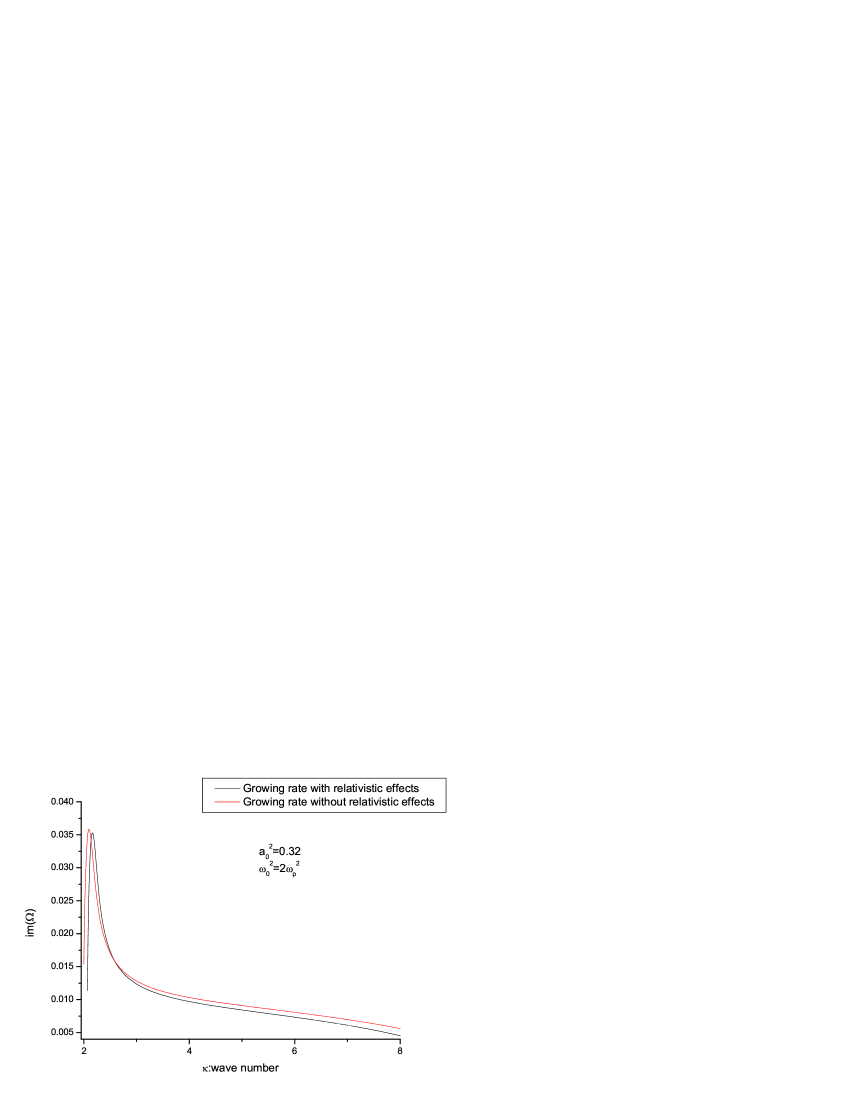
Figure 3: the comparison of relativistic and non-relativistic growing rates.

4 Conclusion

The present paper applied the quasi-periodic approximate method for the stable laser propagation in weak relativistic plasmas. The Stimulated Brillouin Scatter in relativistic region is investigated in detail. The growing rates are re-calculated numerically and the sideband-mixing effects are considered. The Brillouin instability is reduced by these effects. For the plateau region of pure growing modes, the reduction is more evidence.

reference

References

[1]Kruer W L 2000 Phy. Plasmas. 7 2270
[2]Sprangle P, Esarey E, Ting A 1990 Phys. Rev. Lett. 64 2011
[3]Sprangle P, Esarey E, Hafizi B 1997 Phys. Rev. E. 56 5894
[4]Schroeder C B, Esarey E, Shadwick B A,Leemans W P 2003 Phys. Plasmas. 10 285
[5]Hartemann F V etc al 1995 Phys. Rev. E. 51 4833
[6]Rubenchik A, Witkowski S 1991 Physics of Laser Plasma (Amsterdam
Elsevier Science Publishers)
[7]Hafizi B, Ting A, Sprangle P,Hubbard R F 2000 Phy. Rev. E. 62 4210
[8]Satyabrata Kar, Tripathi V K, Sawhney B K 2002 Phys. Plasmas. 9 576
[9]Mahmoud S T, Sharma R P 2001 Phy. Plasmas. 8 3419
[10]Antonsen T M, Mora P 1993 Phy. Plasma, 5 1440
[11]Antonsen T M, Mora P 1992 Phys. Rev. Lett. 69 2204
[12]Sprangle P, Esarey E, Hafizi B 1997 Phys. Rev. Lett. 79 1046
[13]Sprangle P, Essarey E, Krall J, Jopyce G 1992 Phys. Rev. Lett. 69 2200
[14]Kruer W L 1986 The Physics of Laser Plasma Interactions (Redwood City Addison-Wesley)
[15]Wang X F, Fedosejevs R, Tsakiris G D 1998 Opt. Commun. 146 363