Extending Granger causality to nonlinear systems

Abstract

We consider extension of Granger causality to nonlinear bivariate time series. In this frame, if the prediction error of the first time series is reduced by including measurements from the second time series, then the second time series is said to have a causal influence on the first one. Not all the nonlinear prediction schemes are suitable to evaluate causality, indeed not all of them allow to quantify how much the knowledge of the other time series counts to improve prediction error. We present a novel approach with bivariate time series modelled by a generalization of radial basis functions and show its application to a pair of unidirectionally coupled chaotic maps and to a physiological example.

I Introduction

Identifying causal relations among simultaneously acquired signals is an important problem in computational time series analysis and has applications in economy [1-2], EEG analysis tass , human cardiorespiratory system cardioresp , interaction between heart rate and systolic arterial pressure akselrod , and many others. Several papers dealt with this problem relating it to the identification of interdependence in nonlinear dynamical systems arnold , or to estimates of information rates schreiber ; palus . Some approaches modelled data by oscillators and concentrated on the phases of the signals rosemblum . One major approach to analyze causality between two time series is to examine if the prediction of one series could be improved by incorporating information of the other, as proposed by Granger granger in the context of linear regression models of stochastic processes. In particular, if the prediction error of the first time series is reduced by including measurements from the second time series in the linear regression model, then the second time series is said to have a causal influence on the first time series. By exchanging roles of the two time series, one can address the question of causal influence in the opposite direction. It is worth stressing that, within this definition of causality, flow of time plays a major role in making inference, from time series data, depending on direction. Since Granger causality was formulated for linear models, its application to nonlinear systems may not be appropriate. The question we address in this paper is: how is it possible to extend Granger causality definition to nonlinear problems?

In the next section we review the original approach by Granger while describing our point of view about its nonlinear extension; we also propose a method, exploiting radial basis functions, which fulfills the requirements a prediction scheme should satisfy to analyze causality. In section (III) we show application of the proposed method to simulated and real examples. Some conclusions are drawn in Section (IV).

II Granger causality

II.1 Linear modelling of bivariate time series.

We briefly recall the Vector AutoRegressive (VAR) model which is used to define linear Granger causality granger . Let $\{\bar{x}_{i}\}_{i=1,.,N}$ and $\{\bar{y}_{i}\}_{i=1,.,N}$ be two time series of $N$ simultaneously measured quantities. In the following we will assume that time series are stationary. For $k=1$ to $M$ (where $M=N-m$, $m$ being the order of the model), we denote $x^{k}=\bar{x}_{k+m}$, $y^{k}=\bar{y}_{k+m}$, ${\bf X}^{k}=(\bar{x}_{k+m-1},\bar{x}_{k+m-2},...,\bar{x}_{k})$, ${\bf Y}^{k}=(\bar{y}_{k+m-1},\bar{y}_{k+m-2},...,\bar{y}_{k})$ and we treat these quantities as $M$ realizations of the stochastic variables ($x$, $y$, ${\bf X}$, ${\bf Y}$). The following model is then considered nota1 :

$$\begin{array}[]{l}x={\bf W_{11}}\cdot{\bf X}+{\bf W_{12}}\cdot{\bf Y},\\ y={\bf W_{21}}\cdot{\bf X}+{\bf W_{22}}\cdot{\bf Y},\end{array}$$ (3)

$\{{\bf W}\}$ being four $m$-dimensional real vectors to be estimated from data. Application of least squares techniques yields the solutions:

$$\left(\begin{array}[]{c}{\bf W_{11}}\\ {\bf W_{12}}\end{array}\right)=\left(\begin{array}[]{cc}\Sigma_{xx}&\Sigma_{xy}\\ \Sigma_{yx}&\Sigma_{yy}\end{array}\right)^{-1}\left(\begin{array}[]{c}{\bf T_{11}}\\ {\bf T_{12}}\end{array}\right),$$

and

$$\left(\begin{array}[]{c}{\bf W_{21}}\\ {\bf W_{22}}\end{array}\right)=\left(\begin{array}[]{cc}\Sigma_{xx}&\Sigma_{xy}\\ \Sigma_{yx}&\Sigma_{yy}\end{array}\right)^{-1}\left(\begin{array}[]{c}{\bf T_{21}}\\ {\bf T_{22}}\end{array}\right),$$

where $\Sigma$ matrices and $T$ vectors are the estimates, based on the data set at hand, of the following average values:

$$\begin{array}[]{lll}\left[\Sigma_{xx}\right]_{\alpha\beta}=\langle X_{\alpha}X_{\beta}\rangle&={1\over M}\sum_{k=1}^{M}X_{\alpha}^{k}X_{\beta}^{k}&\alpha,\beta=1,...,m\\ \left[\Sigma_{xy}\right]_{\alpha\beta}=\langle X_{\alpha}Y_{\beta}\rangle&={1\over M}\sum_{k=1}^{M}X_{\alpha}^{k}Y_{\beta}^{k}&\alpha,\beta=1,...,m\\ \left[\Sigma_{yx}\right]_{\alpha\beta}=\langle Y_{\alpha}X_{\beta}\rangle&={1\over M}\sum_{k=1}^{M}Y_{\alpha}^{k}X_{\beta}^{k}&\alpha,\beta=1,...,m\\ \left[\Sigma_{yy}\right]_{\alpha\beta}=\langle Y_{\alpha}Y_{\beta}\rangle&={1\over M}\sum_{k=1}^{M}Y_{\alpha}^{k}Y_{\beta}^{k}&\alpha,\beta=1,...,m\\ \left[{\bf T_{11}}\right]_{\alpha}=\langle xX_{\alpha}\rangle&={1\over M}\sum_{k=1}^{M}x^{k}X_{\alpha}^{k}&\alpha=1,...,m\\ \left[{\bf T_{12}}\right]_{\alpha}=\langle xY_{\alpha}\rangle&={1\over M}\sum_{k=1}^{M}x^{k}Y_{\alpha}^{k}&\alpha=1,...,m\\ \left[{\bf T_{21}}\right]_{\alpha}=\langle yX_{\alpha}\rangle&={1\over M}\sum_{k=1}^{M}y^{k}X_{\alpha}^{k}&\alpha=1,...,m\\ \left[{\bf T_{22}}\right]_{\alpha}=\langle yY_{\alpha}\rangle&={1\over M}\sum_{k=1}^{M}y^{k}Y_{\alpha}^{k}&\alpha=1,...,m\par\end{array}$$ (12)

Let us call $\epsilon_{xy}$ and $\epsilon_{yx}$ the prediction errors of this model, defined as the estimated variances of $x-{\bf W_{11}}\cdot{\bf X}-{\bf W_{12}}\cdot{\bf Y}$ and $y-{\bf W_{21}}\cdot{\bf X}-{\bf W_{22}}\cdot{\bf Y}$ respectively. In particular

$$\begin{array}[]{l}\epsilon_{xy}={1\over M}\sum_{k=1}^{M}(x^{k}-{\bf W_{11}}\cdot{\bf X}^{k}-{\bf W_{12}}\cdot{\bf Y}^{k})^{2};\\ \epsilon_{yx}={1\over M}\sum_{k=1}^{M}(y^{k}-{\bf W_{21}}\cdot{\bf X}^{k}-{\bf W_{22}}\cdot{\bf Y}^{k})^{2}.\end{array}$$ (15)

We also consider AutoRegressive (AR) predictions of the two time series, i.e. the model

$$\begin{array}[]{l}x={\bf V_{1}}\cdot{\bf X},\\ y={\bf V_{2}}\cdot{\bf Y}.\end{array}$$ (18)

In this case the least squares approach provides ${\bf V_{1}}=\Sigma_{xx}^{-1}{\bf T_{11}}$ and ${\bf V_{2}}=\Sigma_{yy}^{-1}{\bf T_{22}}$. The estimate of the variance of $x-{\bf V_{1}}\cdot{\bf X}$ is called $\epsilon_{x}$ (the prediction error when $x$ is predicted solely on the basis of the knowledge of its past values); similarly $\epsilon_{y}$ is the variance of $y-{\bf V_{2}}\cdot{\bf Y}$. If the prediction of $x$ improves by incorporating the past values of $\{y_{i}\}$, i.e. $\epsilon_{xy}$ is smaller than $\epsilon_{x}$, then $y$ has a causal influence on $x$. Analogously, if $\epsilon_{yx}$ is smaller than $\epsilon_{y}$, then $x$ has a causal influence on $y$. Calling $c_{1}=\epsilon_{x}-\epsilon_{xy}$ and $c_{2}=\epsilon_{y}-\epsilon_{yx}$, a directionality index can be introduced:

$$D={c_{2}-c_{1}\over c_{1}+c_{2}}.$$ (19)

The index $D$ varies from $1$ in the case of unidirectional influence ($x\to y$) to $-1$ in the opposite case ($y\to x$), with intermediate values corresponding to bidirectional influence. According to this definition of causality, the following property holds for $N$ sufficiently large: if ${\bf Y}$ is uncorrelated with ${\bf X}$ and $x$, then $\epsilon_{x}=\epsilon_{xy}$. Indeed in this case $\Sigma_{xy}=\Sigma_{yx}=0$ and ${\bf T_{12}}=0$, therefore ${\bf W_{12}}=0$. This means that VAR and AR modelling of the $\{x_{i}\}$ time series coincide. Analogously if ${\bf X}$ is uncorrelated with ${\bf Y}$ and $y$, then $\epsilon_{y}=\epsilon_{yx}$. It is clear that these properties are fundamental and make the linear prediction approach suitable to evaluate causality. On the other hand, for nonlinear systems higher order correlations may be relevant. Therefore, we propose that any prediction scheme providing a nonlinear extension of Granger causality should satisfy the following property: (P1) if ${\bf Y}$ is statistically independent of ${\bf X}$ and $x$, then $\epsilon_{x}=\epsilon_{xy}$; if ${\bf X}$ is statistically independent of ${\bf Y}$ and $y$, then $\epsilon_{y}=\epsilon_{yx}$. In a recent paper chen , use of a locally linear prediction scheme farmer has been proposed to evaluate nonlinear causality. In this scheme, the joint dynamics of the two time series is reconstructed by delay vectors embedded in an Euclidean space; in the delay embedding space a locally linear model is fitted to data. The approach described in chen satisfies property P1 only if the number of points in the neighborhood of each reference point, where linear fit is done, is sufficiently high to establish good statistics; however linearization is valid only for small neighborhoods. It follows that this approach to nonlinear causality requires very long time series to satisfy P1. In order to construct methods working effectively with moderately long time series, in the next subsection we will characterize the problem of extending Granger causality as the one of finding classes of nonlinear models satisfying property P1.

II.2 Nonlinear models.

What is the most general class of nonlinear models which satisfy P1? The complete answer to this question is matter for further study. Here we only give a partial answer, i.e. the following family of models:

$$\begin{array}[]{l}x={\bf w_{11}}\cdot{\bf\Phi}\left({\bf X}\right)+{\bf w_{12}}\cdot{\bf\Psi}\left({\bf Y}\right),\\ y={\bf w_{21}}\cdot{\bf\Phi}\left({\bf X}\right)+{\bf w_{22}}\cdot{\bf\Psi}\left({\bf Y}\right),\end{array}$$ (22)

where $\{\bf w\}$ are four $n$-dimensional real vectors, ${\bf\Phi}=\left(\varphi_{1},...,\varphi_{n}\right)$ are $n$ given nonlinear real functions of $m$ variables, and ${\bf\Psi}=\left(\psi_{1},...,\psi_{n}\right)$ are $n$ other real functions of $m$ variables. Given ${\bf\Phi}$ and ${\bf\Psi}$, model (22) is a linear function in the space of features $\varphi$ and $\psi$; it depends on $4n$ variables, the vectors $\{\bf w\}$, which must be fixed to minimize the prediction errors

$$\begin{array}[]{l}\epsilon_{xy}={1\over M}\sum_{k=1}^{M}(x^{k}-{\bf w_{11}}\cdot{\bf\Phi}\left({\bf X}^{k}\right)-{\bf w_{12}}\cdot{\bf\Psi}\left({\bf Y}^{k}\right))^{2};\\ \epsilon_{yx}={1\over M}\sum_{k=1}^{M}(y^{k}-{\bf w_{21}}\cdot{\bf\Phi}\left({\bf X}^{k}\right)-{\bf w_{22}}\cdot{\bf\Psi}\left({\bf Y}^{k}\right))^{2}.\end{array}$$ (25)

We also consider the model:

$$\begin{array}[]{l}x={\bf v_{1}}\cdot{\bf\Phi}\left({\bf X}\right),\\ y={\bf v_{2}}\cdot{\bf\Psi}\left({\bf Y}\right),\end{array}$$ (28)

and the corresponding prediction errors $\epsilon_{x}$ and $\epsilon_{y}$.

Now we prove that model (22) satisfies P1. Let us suppose that ${\bf Y}$ is statistically independent of ${\bf X}$ and $x$. Then, for each $\mu=1,..,n$ and for each $\lambda=1,..,n$: $\psi_{\mu}\left({\bf Y}\right)$ is uncorrelated with $x$ and with $\varphi_{\lambda}\left({\bf X}\right)$. It follows that

$$\mbox{variance}\left[x-{\bf w_{11}}\cdot{\bf\Phi}\left({\bf X}\right)-{\bf w_{12}}\cdot{\bf\Psi}\left({\bf Y}\right)\right]=\mbox{variance}\left[x-{\bf w_{11}}\cdot{\bf\Phi}\left({\bf X}\right)\right]+\mbox{variance}\left[{\bf w_{12}}\cdot{\bf\Psi}\left({\bf Y}\right)\right].$$ (29)

As a consequence, for large $N$, at the minimum of $\epsilon_{xy}$ one has ${\bf w_{12}}=0$. The same argument may be used exchanging x and y. This proves that P1 holds.

The solution of least squares fitting of model (22) to data may be written in the following form:

$$\left(\begin{array}[]{c}{\bf w_{11}}\\ {\bf w_{12}}\end{array}\right)=\left({\bf S_{1}}\;\;\;{\bf S_{2}}\right)^{\dagger}{\bf t_{1}},$$

$$\left(\begin{array}[]{c}{\bf w_{21}}\\ {\bf w_{22}}\end{array}\right)=\left({\bf S_{2}}\;\;\;{\bf S_{1}}\right)^{\dagger}{\bf t_{2}},$$

where ^† denotes the pseudo-inverse matrix rao ; ${\bf S}$ matrices and ${\bf t}$ vectors are given by:

$$\begin{array}[]{ll}\left[{\bf S_{1}}\right]_{k\rho}=\varphi_{\rho}\left({\bf X}^{k}\right)&k=1,...,M,\rho=1,...,n\\ \left[{\bf S_{2}}\right]_{k\rho}=\psi_{\rho}({\bf Y}^{k})&k=1,...,M,\rho=1,...,n\\ \left[{\bf t_{1}}\right]_{k}=x^{k}&k=1,...,M\\ \left[{\bf t_{2}}\right]_{k}=y^{k}&k=1,...,M\end{array}$$ (34)

Solution of model (28) is given by ${\bf v_{1}}={\bf S_{1}}^{\dagger}{\bf t_{1}}$ and ${\bf v_{2}}={\bf S_{2}}^{\dagger}{\bf t_{2}}$.

II.3 Radial basis functions.

Radial basis functions (RBF) methods were initially proposed to perform exact interpolation of a set of data points in a multidimensional space (see, e.g., bishop ); subsequently an alternative motivation for RBF methods was found within regularization theory poggio . RBF models have been used to model financial time series hutch .

In this subsection we propose a strategy to choose the functions ${\bf\Phi}$ and ${\bf\Psi}$, in model (22), in the frame of RBF methods. Fixed $n\ll M$, $n$ centers $\{{\bf\tilde{X}}^{\rho}\}_{\rho=1}^{n}$, in the space of ${\bf X}$ vectors, are determined by a clustering procedure applied to data $\{{\bf X}^{k}\}_{k=1}^{M}$. Analogously $n$ centers $\{{\bf\tilde{Y}}^{\rho}\}_{\rho=1}^{n}$, in the space of ${\bf Y}$ vectors, are determined by a clustering procedure applied to data $\{{\bf Y}^{k}\}_{k=1}^{M}$. We then make the following choice:

$$\begin{array}[]{ll}\varphi_{\rho}\left({\bf X}\right)=\exp\left({-\|{\bf X}-{\bf\tilde{X}}^{\rho}\|^{2}/2\sigma^{2}}\right)&\rho=1,...,n,\\ \psi_{\rho}\left({\bf Y}\right)=\exp\left({-\|{\bf Y}-{\bf\tilde{Y}}^{\rho}\|^{2}/2\sigma^{2}}\right)&\rho=1,...,n,\end{array}$$ (37)

$\sigma$ being a fixed parameter, whose order of magnitude is the average spacing between the centers. Centers $\{{\bf\tilde{X}}^{\rho}\}$ are the prototypes of ${\bf X}$ variables, hence $\varphi$ functions measure the similarity to these typical patterns. Analogously, $\psi$ functions measure the similarity to typical patterns of ${\bf Y}$. Many clustering algorithm may be applied to find prototypes, for example in our experiments we use fuzzy c-means fcm .

Some remarks are in order. First, we observe that the models described above may trivially be adapted to handle the case of reconstruction embedding of the two time series in a delay coordinate space, as described in chen . Second, we stress that in (22) $x$ and $y$ are modelled as the sum of two contributions, one depending solely on ${\bf X}$ and the other dependent on ${\bf Y}$. Obviously better prediction models for $x$ and $y$ exists, but they would not be useful to evaluate causality unless they would satisfy P1. This requirement poses a limit to the level of detail at which the two time series may be described, if one is looking at causality relationships. The justification of the model we propose here, based on regularization theory, is sketched in the Appendix.

II.4 Empirical risk and generalization error.

In the previous subsections the prediction error has been identified as the empirical risk, although there is a difference between these two quantities as Statistical Learning Theory (SLT) vapnik-book-1998 shows. The deep connection between empirical risk and generalization error deserves a comment here. First of all we want to point out that the ultimate goal of a predictor and in general of any supervised machine $x=f({\bf X})$ nota2 is to generalize, that is to correctly predict the output values $x$ corresponding to never seen before input patterns ${\bf X}$ (for definiteness we consider the case of predicting $x$ on the basis of the knowledge of ${\bf X}$). A measure of the generalization error of such a machine $f$ is the risk $R[f]$ defined as the expected value of the loss function $V\left(x,f({\bf X})\right)$:

$$R[f]=\int dx\;d{\bf X}\;\;V\left(x,f({\bf X})\right)P(x,{\bf X}),$$ (38)

where $P(x,{\bf X})$ is the probability density function underlying the data. A typical example of loss function is $V\left(x,f({\bf X})\right)=\left(x-f({\bf X})\right)^{2}$ and in this case the function minimizing $R[f]$ is called the regression function. In general $P$ is unknown and so we can not minimize the risk. The only data we have are $M$ observations (examples) $S=\{(x^{k},{\bf X}^{k})\}_{k=1}^{M}$ of the random variables $x$ and ${\bf X}$ drawn according to $P(x,{\bf X})$. Statistical learning theory vapnik-book-1998 as well as regularization theory poggio provide upper bounds of the generalization error of a learning machine $f$. Inequalities of the following type may be proven:

$$R[f]\leq\epsilon_{x}+{\cal C},$$ (39)

where

$$\epsilon_{x}={1\over M}\sum_{k=1}^{M}\left(x^{k}-f({\bf X}^{k})\right)^{2}$$ (40)

is the empirical risk, that measures the error on the training data. ${\cal C}$ is a measure of the complexity of machine $f$ and it is related to the so-called Vapnik-Chervonenkis (VC) dimension. Predictors with low complexity guarantee low generalization error because they avoid overfitting to occur. When the complexity of the functional space where our predictor lives is small, then the empirical risk is a good approximation of the generalization error. The models we deal with in this work verify such constraint. In fact, linear predictors have a finite VC-dimension, equal to the size of the space where the input patterns live, and predictors expressed as linear combinations of radial basis functions are smooth. In conclusion empirical risk is a good measure of the generalization error for the predictors we are considering here and so it can be used to construct measures of causality between time series loo .

III Experiments.

In order to demonstrate the use of the proposed approach, in this section we study two examples, a pair of unidirectionally coupled chaotic maps and a bivariate physiological time series.

III.1 Chaotic maps.

Let us consider the following pair of noisy logistic maps:

$$\begin{array}[]{l}x_{n+1}=a\;x_{n}\;\left(1-x_{n}\right)+s\eta_{n+1},\\ y_{n+1}=e\;a\;y_{n}\;\left(1-y_{n}\right)+(1-e)\;a\;x_{n}\;\left(1-x_{n}\right)+s\xi_{n+1};\end{array}$$ (43)

$\{\eta\}$ and $\{\xi\}$ are unit variance Gaussianly distributed noise terms; parameter $s$ determines their relevance. We fix $a=3.8$, and $e\in[0,1]$ represents the coupling $x\to y$. In the noise-free case ($s=0$), a transition to synchronization ($x_{n}=y_{n}$) occurs at $e=0.37$. We evaluate the Lyapunov exponents by the method described in bremen : the first exponent is $0.43$, the second exponent depends on $e$ and is depicted in Fig. 1 for $e<0.37$ (it becomes negative for $e>0.37$). For several values of $e$, we have considered runs of $10^{5}$ iterations, after $10^{5}$ transient, and evaluated the prediction errors by (22) and (28), with $m=1$, $n=100$ and $\sigma=0.05$. In fig. 2a we depict, in the noise free case, the curves representing $c_{1}$ and $c_{2}$ versus coupling $e$. In figures 2b, 2c and 2d we depict the directionality index $D$ versus $e$, in the noise free case and for $s=0.01$ and $s=0.07$ respectively. In the noise free case we find $D=1$, i.e. our method revealed unidirectional influence. As the noise increases, also the minimum value of $e$, which renders unidirectional coupling detectable, increases.

III.2 Physiological data.

As a real example, we consider time series of heart rate and breath rate of a sleeping human suffering from sleep apnea (ten minutes from data set B of the Santa Fe Institute time series contest held in 1991, available in the Physionet data bank physionet ). There is a growing evidence that suggests a causal link between sleep apnea and cardiovascular disease roux , although the exact mechanisms that underlie this relationship remain unresolved somno . Figure 3 clearly shows that bursts of the patient breath and cyclical fluctuations of heart rate are interdependent. We fix $m=1$ and $n=50$; varying $\sigma$ we find that both $\epsilon_{x}$ ($x$ representing heart rate) and $\epsilon_{y}$ ($y$ representing breath) have a minimum at $\sigma$ close to $0.5$. In fig. 4 we depict the directionality index $D$ vs $\sigma$, around $\sigma=0.5$. Since we find $D$ positive, we may conclude that the causal influence of heart rate on breath is stronger than the reverse nota3 . This data have been already analyzed in schreiber , measuring the rate of information flow (transfer entropy), and a stronger flow of information from the heart rate to the breath rate was found. In this example, the rate of information flow entropy and Granger nonlinear causality give consistent results: both these quantities, in the end, measure the departure from the generalized Markov property schreiber

$$\begin{array}[]{ll}P(x\;|\;{\bf X})\;=\;P(x\;|\;{\bf X},{\bf Y}),\\ P(y\;|\;{\bf Y})\;=\;P(y\;|\;{\bf X},{\bf Y}).\end{array}$$ (46)

IV Conclusions.

The components of complex systems in nature rarely display a linear interdependence of their parts: identification of their causal relationships provides important insights on the underlying mechanisms. Among the variety of methods which have been proposed to handle this important task, a major approach was proposed by Granger granger . It is based on the improvement of predictability of one time series due to the knowledge of the second time series: it is appealing for its general applicability, but is restricted to linear models. While extending Granger approach to the nonlinear case, on one hand one would like to have the most accurate modelling of the bivariate time series, on the other hand the goal is to quantify how much the knowledge of the other time series counts to reach this accuracy. Our analysis is rooted on the fact that any nonlinear modelling of data, suitable to study causality, should satisfy the property P1, described in Section (II). It is clear that this property sets a limit on the accuracy of the model; we have proposed a class of nonlinear models which satisfy P1 and constructed an RBF like approach to nonlinear Granger causality. Its performances, in a simulated case and a real physiological application, have been presented. We conclude remarking that use of this definition of nonlinear causality may lead to discover genuine causal structures via data analysis, but to validate the results the analysis has to be accompanied by substantive theory.

Acknoledgements. The authors thank Giuseppe Nardulli and Mario Pellicoro for useful discussions about causality.

V Appendix.

We show how the choice of functions (37) arise in the frame of regularization theory. Let $z$ be a function of ${\bf X}$ and ${\bf Y}$. We assume that $z$ is the sum of a term depending solely on ${\bf X}$ and one depending on ${\bf Y}$: $z({\bf X},{\bf Y})=f({\bf X})+g({\bf Y})$. We also assume the knowledge of the values of $f$ and $g$ at points $\{{\bf\tilde{X}}^{\rho},{\bf\tilde{Y}}^{\rho}\}_{\rho=1,..,n}$:

$$\begin{array}[]{ll}f({\bf\tilde{X}}^{\rho})=f^{\rho}&\rho=1,...,n,\\ g({\bf\tilde{Y}}^{\rho})=g^{\rho}&\rho=1,...,n.\\ \end{array}$$ (49)

Let us denote $\hat{K}(\vec{\omega})$ the Fourier transform of $K(\vec{r})=\exp(-r^{2}/2\sigma^{2})$. The following functional is a measure of the smoothness of z(X,Y):

$${\cal S}[z]=\int d\vec{\omega}\;\;{|\hat{f}(\vec{\omega})|^{2}+|\hat{g}(\vec{\omega})|^{2}\over\hat{K}(\vec{\omega})}.$$ (50)

Indeed it penalizes functions with relevant contributions from high frequency modes. Variational calculus shows that the function that minimize ${\cal S}$ under the constraints (49) is given by:

$$z=\sum_{\rho=1}^{n}\mu_{\rho}\;K\left({\bf X}-{\bf\tilde{X}}^{\rho}\right)+\sum_{\rho=1}^{n}\lambda_{\rho}\;K\left({\bf Y}-{\bf\tilde{Y}}^{\rho}\right);$$ (51)

where $\{\mu\}$ and $\{\lambda\}$ are tunable Lagrange multipliers to solve (49). Hence model (22)-(37) corresponds to the class of the smoothest functions, sum of a term depending on ${\bf X}$ and a term depending on ${\bf Y}$, with assigned values on a set of $n$ points.

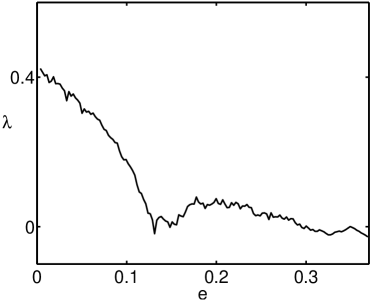
Figure 1: The second Lyapunov exponent of the coupled maps (43) is plotted versus coupling $e$.

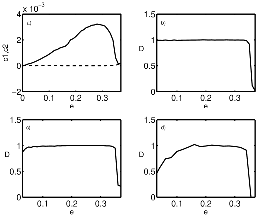
Figure 2: (a) For the noise free case of coupled maps (43), $c_{1}=\epsilon_{x}-\epsilon_{xy}$ (dashed line) and $c_{2}=\epsilon_{y}-\epsilon_{yx}$ (solid line) are plotted versus coupling $e$. (b) The directionality index $D$ (see the text) is plotted versus $e$ in the noise free case. (c) The directionality index $D$ is plotted versus $e$, $s=0.01$. (d) $D$ is plotted versus $e$, $s=0.07$.

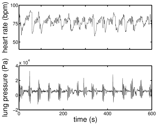
Figure 3: Time series of the heart RR (upper) and breath signal (lower) of a patient suffering sleep apnea. Data sampled at 2 Hz.

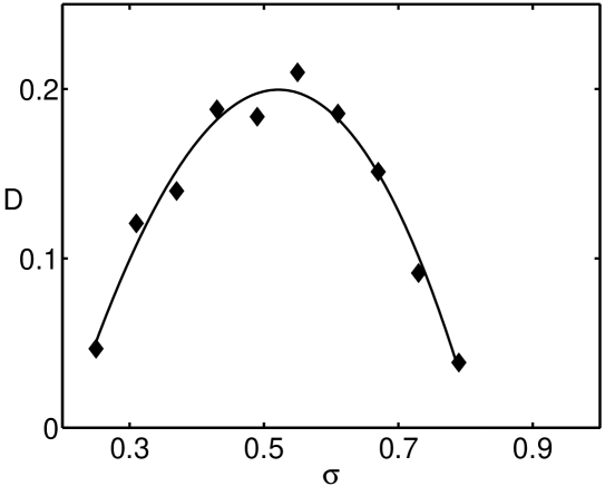
Figure 4: The directionality index $D$ is plotted versus $\sigma$ for the physiological application, around $\sigma=0.5$. Solid line is the $3th$-polynomial best fit of points, here shown only for illustrative purposes.

References

- (1) C.W.J. Granger, Econometrica 37, 424 (1969).
- (2) J.J. Ting, Physica A 324, 285 (2003).
- (3) P. Tass et al., Phys. Rev. Lett. 81, 3291 (1998); M. Le van Quyen et al., Brain Res. 792, 24 (1998); E. Rodriguez et al., Nature (London) 397, 430 (1999).
- (4) C. Ludwig, Arch. Anat. Physiol. 13, 242 (1847); C. Schafer et al., Phys. Rev. E 60, 857 (1999); M. G. Rosemblum et al., Phys. Rev. E 65, 41909 (2002).
- (5) S. Akselrod et al., Am. J. Physiol. Heart. Circ. Physiol. 249, H867 (1985); G. Nollo et al., Am. J. Physiol. Heart. Circ. Physiol. 283, H1200 (2002).
- (6) S. J. Schiff et al., Phys. Rev. E 56, 6708 (1996); J. Arnhold et al., Physica D 134, 419 (1999); R. Quian Quiroga et al., Phys. Rev. E 61, 5142 (2000); R. Quian Quiroga et al., Phys. Rev. E 65, 41903 (2002).
- (7) T. Schreiber, Phys. Rev. Lett. 85, 461 (2000).
- (8) M. Palus et al., Phys. Rev. E 63, 46211 (2001).
- (9) F. R. Drepper, Phys. Rev. E 62, 6376 (2000); M. G. Rosemblum et al., Phys. Rev. E 64, 45202R (2001).
- (10) Usually both times series are normalized in the preprocessing stage, i.e. they are linearly transformed to have zero mean and unit variance.
- (11) Y. Chen et al., Phys. Lett. A 324, 26 (2004).
- (12) J.D. Farmer and J.J. Sidorowich, Phys. Rev. Lett. 59, 845 (1987).
- (13) C. R. Rao and S.K. Mitra, Generalized Inverse of Matrices and Its Applications (John Wiley, New York, 1971).
- (14) C. M. Bishop, Neural networks for pattern recognition (Oxford University Press, New York, 1995).
- (15) T. Poggio, F. Girosi, Science 247, 978 (1990).
- (16) J. Hutchinson, A Radial Basis Function Approach to Financial Time Series Analysis, Ph.D. Thesis, Massachusetts Institute of Technology, Department of Electrical Engineering and Computer Science (1994).
- (17) J. C. Bezdek, Pattern Recognition with Fuzzy Objective Function Algorithms (Plenum Press, New York, 1981).
- (18) V. Vapnik, Statistical Learning Theory (John Wiley & Sons, INC., 1998).
- (19) Machine means ’algorithm which learns from data’ in the machine learning community.
- (20) In the general case, Leave-one-out (Loo) error provides a better estimate of the generalization error of (Luntz and Brailovsky theorem) than the empirical risk, given a finite number of training data. Loo-error is defined as the error variance when the prediction for the k-th pattern is made using the model trained on the M-1 other patterns; it needs predictors to be trained, where is the cardinality of the data set. Hence, Loo-error estimation is unfeasible to compute for large training sets. For linear predictors, like the ones we consider in this paper, the empirical risk is already a good estimate, due to the low complexity of these machines.
- (21) H. F. von Bremen et al., Physica D 101, 1 (1997).
- (22) http://www.physionet.org/
- (23) F. Roux et al., Am. J. Med. 108, 396 (2000).
- (24) H. W. Duchna et al., Somnologie 7, 101 (2003).
- (25) These results may also be due to coupling of the two signals to a common external driver.