MaxEnt assisted MaxLik tomography

Abstract

Maximum likelihood estimation is a valuable tool often applied to inverse problems in quantum theory. Estimation from small data sets can, however, have non unique solutions. We discuss this problem and propose to use Jaynes maximum entropy principle to single out the most unbiased maximum-likelihood guess.

1 Introduction

The role of the variational principles in science can hardly be overemphasized. Maximization or minimization of the appropriate functionals provides elegant solutions of rather complicated problems and contributes to the deeper philosophical understanding of the laws of Nature. Minimization of the optical path-Fermat principle or minimization of the action-Hamilton principle are two particular examples of such a treatment in optics and classical mechanics, respectively. In the thermodynamics and statistical physics an appropriate measure which deserves to be maximized was introduced by Boltzmann as entropy $S=-k_{b}\log\Gamma$, where $\Gamma$ denotes the volume in the phase space or the number of distinguishable states. The role of entropy as uncertainty measure in communication and information theory was recognized by Shannon. His definition $S=-\sum_{n}p_{n}\log p_{n}$ is unique in the sense that fulfills reasonable demands put on the information measure associated with a probability distribution $p_{n}$. Particularly, the uncertainty is maximized when all the outcomes are equally likely– the uniform distribution contains the largest amount of uncertainty. Its implications for physical and technical practice were noticed by Jaynes Jaynes , who proposed a variational method known as principle of Maximum Entropy (MaxEnt). According to this rule one should select such a probability distribution which fulfills given constraints and simultaneously maximizes Shannon entropy. This gives the most unbiased solution of the problem consistent with the given observations. On the philosophical level this corresponds to the celebrated Laplace’s Principle of Insufficient Reasoning. It states that if there is no reason to prefer among several possibilities, than the best strategy is to consider them as equally likely and pick up the average. This strategy appeared to be extremely useful in many applications covering the fields of statistical inference, communication problems or pattern recognition frieden .

But entropy is not the only important functional in probability theory The entropic measure known as Kullback-Leibler divergence Kullback or relative entropy $E(\{p_{i}\}|\{q_{i}\})=\sum_{i}p_{i}\log(p_{i}/q_{i})$ bears striking resemblance to the Shannon entropy, however it posses a different interpretation. It quantifies the distance in the statistical sense between two different distributions $p_{i}$ and $q_{i}$. Provided that one party ($p_{i}$ in our notation) are the sampled relative frequencies, the principle of minimum relative entropy coincides with the maximum likelihood (MaxLik) estimation problem fisher ; Helstrom . Similarly to the previous case of MaxEnt principle MaxLik is not a rule that requires justification - it does not need to be proved. At present there are many examples of successful application of this estimation technique for solving inverse problems, or recently, for quantification of such a fragile effect as entanglement.

Though both the celebrated principles, MaxEnt and MaxLik, rely on the notion of entropy, their usage and interpretation differ substantially. Whereas the former one provides the most conservative guess still consistent with the data, the later one is the most optimistic one fitting the given data in the best possible way frieden ; fisher . However, both the methods are suffering by certain drawbacks: MaxLik is capable of dealing with counted noisy data in realistic experiments but its interpretation usually requires a certain cut-off in the parameter space. Otherwise the solution may appear us under-determined. On the other hand, the MaxEnt principle removes this ambiguity by selecting the most unbiased solution, however realistic data may appear as inconsistent due to the fluctuations, and cannot be straightforwardly used as constraints. The purpose of this contribution is to unify both these concepts into a single estimation procedure capable of handling any data, and to provide the most likely and most unbiased solution without any cut-offs.

2 Maximum-likelihood quantum-state reconstruction

To address the problem of quantum state reconstruction VR ; St ; SBRF93 ; Ulf ; Welsch ; buzek ; banaszek let us consider a generic quantum measurement. The formulation will be developed for the case of finite dimensional quantum systems. The reader can think of a spin 1/2 system for the sake of simplicity.

Assume that we are given a finite number $N$ of identical samples of the system, each in the same but unknown quantum state described by the density operator $\rho$. Given those systems our task is to identify the unknown true state $\rho$ as accurately as possible from the results of measurements performed on them.

On most general level any set of measurements can be represented by a Probability Operator Valued Measure (POVM), $\{\Pi_{j}\},\,j=1\ldots M$. Its elements are semi-positive definite operators that sum up to unity operator, $\Pi_{j}\geq 0,\,\forall j$, $\sum_{j}\Pi_{j}=\hat{1}$. The last requirement is simply the consequence of the conservation of probability: The measured particle is always detected in one of the $M$ output channels, no particles are lost.

Let us assume, for concreteness, that $N$ particles prepared in the same state have been observed in $M$ different output channels of the measurement apparatus. For spin 1/2 particles those channels could be for instance the six output channels of a Stern-Gerlach apparatus subsequently oriented along $x$, $y$, and $z$ directions.

Provided that each particular output

$$\Pi_{j},\qquad j=1,\dots,M$$ (1)

has been registered $n_{j}$ times, $\sum_{j}n_{j}=N,$ the relative frequencies are given as $f_{j}=n_{j}/N.$ Using this data, the true state $\rho$ is to be inferred. The probabilities of occurrences of various outcomes are predicted by quantum mechanics as

$$p_{j}=\mathrm{Tr}\rho\Pi_{j},\quad j=1\ldots M$$ (2)

If the probabilities $p_{j}$ of getting a sufficient number of different outcomes $\Pi_{j}$ were known, it would be possible to determine the true state $\rho$ directly by inverting the linear relation (2). This is the philosophy behind the “standard” quantum tomographic techniques VR ; Ulf . For example, in the rather trivial case of a spin one half particle, the probabilities of getting three linearly independent projectors determine the unknown state uniquely. Here, however, a serious problem arises. Since only a finite number of systems can be investigated, there is no way how to find out those probabilities. The only data one has at his or her disposal are the relative frequencies $f_{j}$, which sample the principally unknowable probabilities $p_{j}$. It is obvious that for a small number of runs, the true probabilities $p_{j}$ and the corresponding detected frequencies $f_{j}$ may differ substantially. As a result of this, the modified realistic problem,

$$f_{j}=\mathrm{Tr}\Pi_{j}\rho$$ (3)

has generally no solution on the space of semi-positive definite hermitian operators describing physical states. This linear equation for the unknown density matrix may be solved for example by means of pattern functions, see e.g. Ulf ; Welsch , what could be considered as a typical example of the standard approach suffering from the above mentioned drawbacks.

Having measurements done and their results registered, the experimenter’s knowledge about the measured system is increased. Since quantum theory is probabilistic, it has little sense to ask the question: ”What quantum state is determined by that measurement?” More appropriate question is Bayes-class ; Bayes-quant ; zdenek_fund ; zdenek_nelin : ”What quantum states seem to be most likely for that measurement?”

Quantum theory predicts the probabilities of individual detections, see Eq. (2). From them one can construct the total joint probability of registering data $\{n_{j}\}$. We assume that the input system (particle) is always detected in one of $M$ output channels, and this is repeated $N$ times. Subsequently, the overall statistics of the experiment is multinomial,

$${\cal L}(\rho)=\frac{N!}{\prod_{i}n_{i}!}\prod_{j}\bigl{[}\mathrm{Tr}(\rho\Pi_{j})\bigr{]}^{n_{j}},$$ (4)

where $n_{j}=Nf_{j}$ denotes the rate of registering a particular outcome $j$. In the following we will omit the multinomial factor from expression (4) as it has no influence on the results. Physically, the quantum state reconstruction corresponds to a synthesis of various measurements done under different experimental conditions, performed on the ensemble of identically prepared systems. For example, the measurement might be subsequent recording of an unknown spin of the neutron (polarization of the photon) using different settings of the Stern Gerlach apparatus, or the recording of the quadrature operator of light in rotated frames in quantum homodyne tomography. The likelihood functional ${\cal L}(\rho)$ quantifies the degree of belief in the hypothesis that for a particular data set $\{n_{j}\}$ the system was prepared in the quantum state $\rho$. The MaxLik estimation simply selects the state for which the likelihood attains its maximum value on the manifold of density matrices.

To make the mathematics simpler we will maximize the logarithm of the likelihood functional,

$$L\propto\sum_{j}f_{j}\log p_{j},$$ (5)

rather then $\mathcal{L}$ itself. Notice that $L$ is a convex functional,

$$L[\alpha\rho_{1}+(1-\alpha)\rho_{2}]\geq\alpha L(\rho_{1})+(1-\alpha)L(\rho_{2}),$$ (6)

defined on the convex set of semi-positive definite density matrices $\rho$, $\rho\geq 0$, $\mathrm{Tr}\rho=1$. This ensures that there is a single global maximum or at most a closed set of equally likely quantum states.

The direct application of the variational principle to likelihood functional together with the convexity property yield the necessary and sufficient condition for its maximum in the form of a nonlinear operator equation Hradil1 ; Rehacek01 ,

$$R\rho=\rho,$$ (7)

where

$$R=\sum_{j}\frac{f_{j}}{p_{j}}\Pi_{j}$$ (8)

is a semi-positive definite operator. In particular, $R$ is unity operator provided the maximum-likelihood solution is strictly positive.

Let us now consider a tomographically incomplete measurement. In such a case, the inverse problem might have multiple solutions. This will happen, for example, when the set of normalized Hermitian operators $\sigma$ satisfying the constraints $p_{j}(\sigma)=f_{j},\,\forall j$ has a nonempty intersection with the set of density matrices. As will be illustrated below, two equally-likely solutions of an under-determined inverse problem can be very different. It is then a question which maximum-likely state should be picked up as the estimate of the true state.

We propose to use Jaynes MaxEnt principle to resolve this ambiguity. Information content of the set of MaxLik solutions can be quantified according to their entropy. A natural choice is then to select the state maximizing the entropy, which is the least biased state with respect to missing measurements.

Let us assume that there are two different density operators $\rho_{1}$ and $\rho_{2}$ maximizing the likelihood functional. The two operators satisfy the extremal equations (7),

$$\begin{split}R(\rho_{1})\rho_{1}&=\rho_{1},\\ R(\rho_{2})\rho_{2}&=\rho_{2}.\end{split}$$ (9)

The interpretation of the operator $R$ is the following: Denoting $f(\rho,\sigma,\alpha)\equiv L[(1-\alpha)\rho+\alpha\sigma]$ the likelihood of a convex combination of states $\rho$ and $\sigma$, and calculating its path derivative at $\rho$,

$$\begin{split}\frac{\partial}{\partial\alpha}f(\rho,\sigma,\alpha)&=\lim\limits_{\alpha\rightarrow 0}\frac{f(\rho,\sigma,\alpha)-f(\rho,\sigma,0)}{\alpha}\\ &=\mathrm{Tr}[R(\rho)\sigma]-1,\end{split}$$ (10)

we see that this derivative is given by the expectation value of $R(\rho)$ taken with $\sigma$. Expectation values of operator $R(\rho)$ define hyperplanes perpendicular to the gradient of the likelihood at $\rho$.

Since the likelihood cannot be increased by moving from $\rho_{1}$ toward $\rho_{2}$ and vice versa (both density matrices are maximum likely states) it follows that

$$\mathrm{Tr}[R(\rho_{1})\rho_{2}]=\mathrm{Tr}[R(\rho_{2})\rho_{1}]=1.$$ (11)

Expressing the two conditions in terms of probabilities $p_{1j}$ and $p_{2j}$ generated by $\rho_{1}$ and $\rho_{2}$, respectively we get

$$\begin{split}&\sum_{j}f_{j}\frac{p_{1j}}{p_{2j}}=1,\\ &\sum_{j}f_{j}\frac{p_{2j}}{p_{1j}}=1,\end{split}$$ (12)

which upon summing the left-hand sides yields condition

$$\sum_{j}f_{j}\frac{p_{1j}^{2}+p_{2j}^{2}}{2p_{1j}p_{2j}}=1.$$ (13)

Now since $(p_{1j}^{2}+p_{2j}^{2})/(2p_{1j}p_{2j})>1$ unless $p_{1j}=p_{2j}$ we obtain,

$$\mathrm{Tr}\rho_{1}\Pi_{j}=\mathrm{Tr}\rho_{2}\Pi_{j},\quad\forall j$$ (14)

which means that the probabilities, and so the operators $R(\rho_{1})$ and $R(\rho_{2})$ are identical. The two extremal equations therefore read,

$$\begin{split}R\rho_{1}&=\rho_{1},\\ R\rho_{2}&=\rho_{2}.\end{split}$$ (15)

Notice that both $\rho_{1}$ and $\rho_{2}$ commute with the common generator $R$.

3 Maximization of entropy

Having found a maximum of the likelihood functional, we still do not know whether this solution is unique or not. Provided a closed set of such states exists, we would like to maximize the entropy functional over it. In this way we will get the least biased maximum-likelihood guess.

The properties of the maximum-likelihood solutions discussed above simplify this problem a lot, because we know that all density matrices belonging to the maximum likely set generate the same probabilities.

We will take those probabilities as constraints of the new optimization problem: Maximize entropy,

$$E(\rho)=-\mathrm{Tr}(\rho\ln\rho),$$ (16)

subject to constraints

$$\mathrm{Tr}(\rho\Pi_{j})=\mathrm{Tr}(\rho_{\mathrm{ML}}\Pi_{j}),\quad j=0\ldots M,$$ (17)

where $\rho_{\mathrm{ML}}$ is a maximum likely state and where we defined $\Pi_{0}=\hat{1}$ to keep the normalization of the estimated state.

Problem Eq. (16) and (17) is known to have a unique solution Jaynes ,

$$\rho_{\mathrm{ME}}=\exp\Bigl{[}\sum_{j}\lambda_{j}\Pi_{j}\Bigr{]},\quad j=0\dots M,$$ (18)

where Lagrange multipliers $\lambda_{j}$ can be determined from the constraints.

The proposed approach combines good features of maximum-likelihood and maximum-entropy methods. From the set of density matrices that are most consistent with the observed data in the sense of maximum likelihood we select the least biased one. At the same time the positivity, and thus also physical soundness, of the result is guaranteed.

Let us remind the reader that a direct application of the maximum entropy principle to raw data (i.e. right hand sides in constraints Eq. (17) replaced by $f_{j}$) is not possible, because the constraints often cannot be satisfied with any semi-positive density operators due to the unavoidable presence of noise in the data.

For the rest of the paper let us restrict ourselves to the most simple case of commuting measurements $[\Pi_{j},\Pi_{k}]=0,\;\forall j,k$. Such tomographic scheme would correspond to the measurement of diagonal elements of the true density matrix. Although this may seem as an oversimplification, many inverse problems can be reduced to this form. Let us mention the neutron absorption tomography, or inefficient photo detection as two significant examples.

4 Example

We will illustrate the proposed reconstruction scheme on a simple example of commuting measurements. Denoting $\{|i\rangle\langle i|\}$ the common eigenbasis of POVM elements $\{\Pi_{j}\}$ we have that

$$\sum_{j}\lambda_{j}\Pi_{j}=\sum_{i}r_{i}|i\rangle\langle i|.$$ (19)

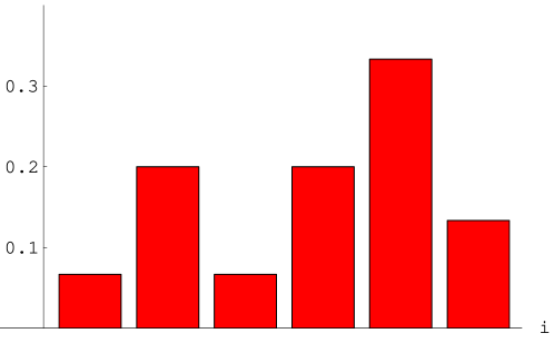
Figure 1: Diagonal representation of a particular true state.

The maximum entropy solution Eq. (18) will assume a diagonal form in this basis, its eigenvalues being,

$$\langle i|\rho_{\mathrm{ME}}|i\rangle=\exp\bigl{[}\sum_{j}\lambda_{j}\langle i|\Pi_{j}|i\rangle\bigr{]}.$$ (20)

Denoting $\rho_{i}=\langle i|\rho|i\rangle$ and $c_{ij}=\langle i|\Pi_{j}|i\rangle$ we finally get a nonlinear system of equations,

$$\sum_{i}e^{\sum_{j^{\prime}}\lambda_{j^{\prime}}c_{ij^{\prime}}}c_{ij}=\sum_{i}c_{ij}\rho_{\mathrm{ML},i}\quad,$$ (21)

that is to be solved for the unknown $M+1$ Lagrange multipliers $\lambda_{j}$.

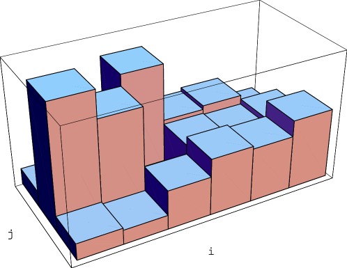
Figure 2: Randomly generated matrix $c_{ij}$ parameterizing a three element POVM.

A particular true six-dimensional vector $\rho_{\mathrm{true},i}$ is shown in Fig. 1. In a simulated experiment this state has been subject to randomly generated three element $POVM$; its elements $c_{ij}$ in the common diagonalizing basis are shown in Fig. 2.

The probabilities of observing results $j=1,2,3$ are as follows: $p_{j}=\sum_{i}c_{ij}\rho_{\mathrm{true},i}$. They are shown in Fig. 3 for our particular choice of $\rho_{\mathrm{true}}$ and $c_{ij}$.

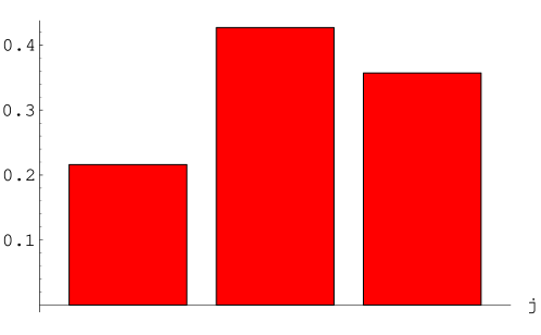
Figure 3: Relative frequencies of the outcomes of a thought tomographic measurement. For the true state and POVM elements, see Figs. 1 and 2.

Taking the probabilities as the input data, we solved the maximum-likelihood extremal equation iteratively starting from three different strictly positive density matrices. It is worth noticing that a quantum state reconstruction from compatible observations is a linear and positive problem. In this case the operator equation (7) reduces to a simple diagonal form which is suitable to iterative solving. This algorithm is sometimes called the expectation maximization algorithm in statistical literature and is known to converge monotonically from any strictly positive initial point dempster ; vardi .

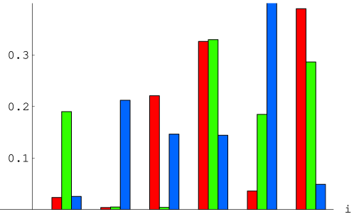
Figure 4: Three particular maximum-likelihood estimates based on the result of the though experiment described in the text.

As we can see, the three maximum-likely estimates represent very different system configurations. The simple POVM used was too rough to resolve those differences, and as a consequence, all the estimated states yield exactly the same probabilities of the three possible outcomes of the measurement.

In the next step, those probabilities were used as constraints for the entropy maximization, as we have discussed in the previous section. As a result, a unique state was selected out of the set of maximum-likely states. The result is shown in Fig. 5.

Figure 5: The result of entropy maximization over the set of maximum-likelihood estimates (three of which are shown in Fig. 4.)

Notice that this state is a good approximation to the original state of Fig. 1. Even though the two are smoothed out a bit, they can be clearly recognized in the reconstruction.

5 Conclusion

We have demonstrated the utility of the maximum-entropy principle for tomographically incomplete quantum state reconstruction schemes. Although the entropic principles cannot be directly applied to noisy experimental data due to the positivity of quantum states, they can be used to remove the ambiguity of maximum likelihood estimation. The proposed method could find applications in quantum homodyne detection and other related infinite-dimensional problems suffering from the lack of experimental data.

References

- (1) Jaynes, E. T., “Information Theory and Statistical Mechanics,” in 1962 Brandeis Summer Lectures, vol. 3, edited by K. W. Ford, Benjamin, New York, 1963, p. 181.
- (2) Frieden, B. R., Probability, Statistical Optics, and Data Testing, Springer-Verlag, Berlin, 1983.
- (3) Kullback, S., and Leibler, R. A., Ann. of Math. Stat., 22, 79 (1951).
- (4) Fisher, R. A., Proc. Camb. Phi. Soc., 22, 700 (1925).
- (5) Helstrom, C. W., Quantum Detection and Estimation Theory, Academic Press, New York, 1976.
- (6) Vogel, K., and Risken, H., Phys. Rev. A, 40, 2847 (1989).
- (7) Weigert, S., Phys. Rev. A, 45, 7688 (1992).
- (8) Smithey, D. T., Beck, M., Raymer, M. G., and Faridani, A., Phys. Rev. Lett., 70, 1244 (1993).
- (9) Leonhardt, U., Measuring of the Quantum State of Light, Cambridge Press, Cambridge, 1997.
- (10) Welsch, D.-G., Vogel, W., and Opatrný, T., “Homodyne Detection and Quantum State Reconstruction,” in Progress in Optics, vol. 39, edited by E. Wolf, North Holland, Amsterdam, 1999.
- (11) Buzek, V., and Derka, R., “Quantum observations,” in Coherence and Statistics of Photons and Atoms, edited by J. Peřina, Wiley, New York, 2001, pp. 198 - 261.
- (12) Banaszek, K., D’Ariano G. M., Paris M. G. A., and Sacchi, M. F., Phys. Rev. A, 61, 010304(R) (1999).
- (13) Bernardo, J. M, and Smith, A. F. M., Bayesian Theory, Wiley, Chichester, 1994.
- (14) Schack, R., Brun, T. A., and Caves, C. M., Phys. Rev. A, 64, 014305 (2001).
- (15) Hradil, Z., and Summhammer, J., J. Phys. A: Math. Gen., 33, 7607 (2000).
- (16) Hradil, Z., Summhammer, J., and Rauch, H., Phys. Lett. A, 261, 20 (1999).
- (17) Hradil, Z., Phys. Rev. A, 55, 1561(R) (1997).
- (18) Řeháček, J., Hradil, Z., and Ježek, M., Phys. Rev. A, 63, 040303(R) (2001).
- (19) Dempster, A. P., Laird, N. M., and Rubin, D. B., J. R. Statist. Soc. B, 39, 1 (1977).
- (20) Vardi Y., and Lee, D., J. R. Statist. Soc. B, 55, 569 (1993).