Data handling, reconstruction, and simulation for the KLOE experiment

Abstract

The broad physics program of the KLOE experiment is based on the high event rate at the Frascati $\phi$ factory, and calls for an up-to-date system for data acquisition and processing. In this review of the KLOE offline environment, the architecture of the data-processing system and the programs developed for data reconstruction and Monte Carlo simulation are described, as well as the various procedures used for data handling and transfer between the different components of the system.

, , , , , , , , , , , , , , , , , , , , , , , , , , , , , , , , , , , , , , , , , , , , , , , , , , , , , , , , , , , , , ,

1 Introduction

KLOE is a general-purpose experiment permanently installed at the Frascati $\phi$ factory, DAΦNE. The KLOE detector was designed for the study of $CP$ violation in the neutral-kaon system. The versatility of the experiment allows for a rich physics program, including measurements of radiative $\phi$ decays, numerous decays of charged and neutral kaons, and measurement of the hadronic cross section, among other topics.

The most interesting channels have branching ratios on the order of $10^{-3}$ or smaller. For precision measurement of these decays, the DAΦNE collider has been designed to achieve a luminosity of $5\times 10^{32}$ $\mathrm{cm}^{-2}\,\mathrm{s}^{-1}$. At this luminosity, the $\phi$ production cross section of about 3 $\mu\mathrm{b}$ translates into an event rate of 1.5 $\mathrm{kHz}$. Bhabha events within the acceptance, together with machine-background and cosmic-ray events, contribute a similar amount to the total acquisition rate. The average KLOE event size is 2.7 $\mathrm{kB}$. We therefore require a data-acquisition (DAQ) system capable of handling a throughput of 10 $\mathrm{MB}/\mathrm{s}$ with high efficiency, a data-processing environment with file servers that provide bandwidth on the order of 100 $\mathrm{MB}/\mathrm{s}$, and a data-storage system capable of handling on the order of a petabyte of data. These numbers are similar to those for other major experiments currently running, and place the design and implementation of the DAQ and offline systems among the more challenging projects in the high-energy physics community.

The high sensitivity needed for the study of $CP$-violation effects and quantum interference patterns in the neutral-kaon system requires that experimental systematics be kept under strict control. To this end, billions of events must be generated, with the most accurate simulation possible of the detector response and machine-background effects.

KLOE data taking for physics began in the year 2000. A total integrated luminosity of about 500 $\mathrm{pb}^{-1}$ was collected by the end of 2002. KLOE data collection is expected to resume at a rate of 10 $\mathrm{pb}^{-1}$/day in 2004.

In this paper, we discuss the KLOE offline data-processing system. We briefly describe the KLOE detector in Sec. 2. The main features of the data-processing environment and the operation of the computer farm are discussed in Sec. 3. The algorithms used in the reconstruction code and their implementation are described in Sec. 4. The KLOE Monte Carlo and its use in event-simulation campaigns is discussed in Sec. 5. In Sec. 6, we summarize and draw some conclusions from our experience.

2 The KLOE detector

For the discrimination of the $CP$-violating decays $K_{L}\to\pi^{+}\pi^{-}$ and $K_{L}\to\pi^{0}\pi^{0}$ from the much more abundant $K_{L}\to\pi\mu\nu$ and $K_{L}\to 3\pi^{0}$ decays, we require of the detector good momentum resolution for charged tracks, as well as full solid-angle coverage and excellent energy and time resolution for photons. Moreover, given the rather long mean decay length of the $K_{L}$ at DAΦNE (3.4 $\mathrm{m}$), a large detector is required in order to have reasonable geometrical acceptance.

The KLOE detector is composed of two subdetectors: a large drift chamber (DC) to measure charged tracks, and an electromagnetic calorimeter (EmC) to detect photons. Both are immersed in the 0.52 $\mathrm{T}$ field of a superconducting solenoid.

The drift chamber [1] is a cylinder of 25 (198) $\mathrm{cm}$ inner (outer) radius and 332 cm length; it contains $12\,582$ drift cells distributed in 58 cylindrical layers. For the 12 inner layers, the cell dimensions are $2\times 2~{}\mathrm{cm}^{2}$, while for the 46 outer layers, they are $3\times 3~{}\mathrm{cm}^{2}$. In order to provide uniform coverage throughout the chamber volume, all wires are stereo wires. The signs of the stereo angles (with respect to the beam axis) alternate from layer to layer, and the magnitude of the stereo angle for each layer gradually increases, from 60 $\mathrm{mrad}$ for the innermost layer to 150 $\mathrm{mrad}$ for the outermost. The total number of wires (sense + field + guard) is about $52\,000$. The spatial resolution in the $r\phi$ plane is about $150~{}\mu\mathrm{m}$; in the $z$ direction, the spatial resolution depends on the stereo angle and is about 2 $\mathrm{mm}$. The chamber is filled with a gas mixture of 90% helium and 10% isobutane. This low-$Z$ mixture has been chosen to reduce the effects of regeneration, photon conversion, and multiple scattering, where the latter has a particularly significant effect on the momentum resolution for tracked particles given the momenta involved in the experiment (100-500 MeV/$c$). The transverse-momentum resolution is $\sigma_{p_{t}}/p_{t}\,\raisebox{-2.58334pt}{$\stackrel{{\scriptstyle\textstyle{<}}}{{\sim}}$}\,0.4\%$ for large-angle tracks. Vertices inside the chamber are reconstructed with a spatial resolution of $\sim$$3$ $\mathrm{mm}$. The chamber was recently instrumented with ADCs to supplement the experiment’s particle-identification capability with $\d E/\d x$ information for reconstructed tracks.

The electromagnetic calorimeter [2] is of the sampling type, and is made of lead layers and scintillating fibers, with a volume proportion of lead:fiber:epoxy = 42:48:10. The total thickness of the EmC is 23 $\mathrm{cm}$, corresponding to about 15 $X_{0}$. The EmC is composed of a barrel and two endcaps. The barrel is divided into 24 modules. Each endcap is divided into 32 (vertical) modules, which have a C shape to close the solid angle as much as possible. The light from the fibers is viewed by a photomultiplier tube (PMT) at each end to determine the time of flight and impact point along the direction of the fibers. The readout is segmented in depth into 5 planes (each 4.4 cm thick, except for the outermost, which is 5.2 cm thick), and in the coordinate transverse to the fibers into columns 4.4 cm wide. In all, there are 4880 PMTs. To complete the coverage of the solid angle, two small calorimeters, QCAL [3], made of lead and scintillating tiles, are wrapped around the low-$\beta$ quadrupoles. The PMT signals (after an electronic delay of about 200 $\mathrm{ns}$) are sent to ADCs for amplitude analysis, to TDCs for time-of-flight measurement, and to the trigger modules. The energy resolution for photons is $\sigma_{E}/E=5.7\%/\surd E(\mbox{GeV})$ and the time resolution is $\sigma_{t}=[54/\surd E(\mbox{GeV})\oplus 50]$ $\mathrm{ps}$. The photon impact point is measured with a precision of $\mbox{$\sim$$1$}~{}\mathrm{cm}/\surd E(\mbox{GeV})$ along the fibers and $\sim$$1$ $\mathrm{cm}$ in the transverse coordinate.

The trigger [4] is based on energy deposits in 88 calorimeter sectors (formed by grouping adjacent readout elements) and on drift-chamber signals. The level-1 trigger, which starts data readout with minimal delay, requires energy deposits above threshold ($E>50$ MeV in the barrel, $E>150$ MeV in the endcaps) in two EmC sectors, or $\sim$$15$ DC wire signals within 250 $\mathrm{ns}$. Low-angle Bhabha events can be downscaled at this level. The level-2 trigger, which validates the level-1 trigger, requires further multiplicity or geometrical conditions for EmC energy deposits, or $\sim$$120$ DC wire signals within a 1.2 $\mu\mathrm{s}$ time window (the maximum drift time is 1–1.5 $\mu\mathrm{s}$, depending on cell size). A cosmic-ray veto is applied at level 2. The acquisition dead time is about 2.7 $\mu\mathrm{s}$ (corresponding to a $0.8\%$ loss at a typical rate of 3 $\mathrm{kHz}$). A level-3 trigger filter is implemented in software to review and enforce the cosmic-ray veto decision made at level 2.

The trigger is synchronized with a demultiplied DAΦNE radio-frequency signal that corresponds to every fourth bunch crossing. ($t_{\mathrm{sync}}=4t_{\mathrm{bunch}}=10.85$ $\mathrm{ns}$). The association of the event with the proper bunch crossing, or determination of the event-start time, is made during offline reconstruction.

The DAQ system [5] handles about $23\,000$ front-end channels (ADC, TDC and trigger modules) hosted in VME crates organized in ten chains. Sub-events from each chain are sent through an FDDI switch to the online farm for event building, formatting, and monitoring. The online farm consists of seven IBM 7026-H50 SMPs, each with four 332-$\mathrm{MHz}$ PowerPC 604e processors. The online servers write the raw-data files to 1.4 $\mathrm{TB}$ of locally mounted SSA disks. The readout system has been designed for a sustained rate of 10 $\mathrm{MB}/\mathrm{s}$. At a typical luminosity of $5\times 10^{31}$ $\mathrm{cm}^{-2}\,\mathrm{s}^{-1}$ during 2002, the trigger rate was 1.6 $\mathrm{kHz}$ and the average event size was 2.7 $\mathrm{kB}$, leading to a sustained data acquisition rate of 4.3 $\mathrm{MB}/\mathrm{s}$, which was managed using three out of seven online nodes.

3 The offline computing environment

Raw data from the online systems are reconstructed on the KLOE offline farm. In this section, we first give an overview of the procedure by which raw data are reconstructed, divided into analysis streams, and then further reduced into data-summary tape (DST) streams. (Monte Carlo production is also performed on the offline farm; the processing of Monte Carlo events is described in Sec. 5.) We then describe the offline hardware environment, the data-handling system (which is common to both the online and offline environments), and the offline software environment.

3.1 Overview of data processing

The event-builder processes running on the online farm write raw events to the online disk pool in 1-$\mathrm{GB}$ files. Data taking is divided into runs of approximately equal integrated luminosity (200 $\mathrm{nb}^{-1}$ in year 2002). Typically, about 20 raw-data files are written per run. For each run, the run number is used to uniquely associate to the events

• a set of calibration constants;

• values for machine parameters such as energy, beam position, etc.;

• quantities related to the detector status such as high- and low-voltage settings, trigger thresholds, drift-chamber gas parameters, dead-channel lists, etc.

All data are permanently stored in a tape library as described in Sec. 3.3. Raw-data files are kept on disk until calibration and reconstruction are completed. The archival of raw-data files and the availability of free space on the online disk pool are managed by the data-handling system as described in Sec. 3.4.

For the drift-chamber calibration [6], two procedures are in use. The first and most commonly used procedure performs a fast analysis to test the validity of the most recent values of the calibration constants. This program runs concurrently with data taking, using cosmic-ray events selected and buffered by the DAQ system. The second procedure performs a complete analysis of cosmic-ray muon tracks in the DC to update the calibration constants; it is launched only if the existing calibrations fail to describe the detector performance. This typically happens only a few times during an entire data-taking period, essentially when the atmospheric pressure changes by more than 1$\%$. The drift-chamber calibration procedures are further described in Sec. 4.2.

For the calorimeter, the calibration procedure [2] is started at the end of each run and lasts about two hours. The procedure uses Bhabha and $\gamma$$\gamma$ events selected by the DAQ system: the 500 MeV photons are used to set the absolute energy and time scales, while the higher-statistics sample of 500 MeV electrons and positrons allows the equalization of the energy scale between different calorimeter columns. With an integrated luminosity of 200 $\mathrm{nb}^{-1}$, the time scale is determined to within 10 $\mathrm{ps}$, and the energy scale is accurate at the percent level.

Various other processes running on the online servers perform on-the-fly reconstruction of selected events to monitor the status of the detector and data-taking conditions (such as hardware efficiencies, noise rates, machine energy, and beam-spot position). The slow-control system combines these data with hardware-status information (such as high- and low-voltage settings and dead-channel maps); it also receives information from the DAΦNE control systems on machine parameters (such as beam currents and number of bunches) and sends information on the status of the experiment to the DAΦNE operators. Monitoring information from all of these sources is summarized and written to the central KLOE database described in Sec. 3.4. Geometry files and calibration constants, as well as some information on long-term detector conditions, are stored using the CERN HEPDB database [7].

Event reconstruction is performed on the offline farm. The reconstruction program datarec starts immediately after the completion of the calibration jobs for the run. Each of the 20 or so raw-data files making up the run are processed in parallel by a separate reconstruction job. Each job produces one reconstructed file for each analysis stream.

In practice, a single job manager periodically interrogates the database, identifies new runs ready for processing, and starts jobs on the free CPUs of the offline farm. The status of these jobs and the overall status of the offline farm itself are monitored via the web interface to the slow-control system. The reconstruction jobs provide additional data-quality and monitoring information, a summary of which is available from the slow-control web interface.

The reconstruction program datarec consists of several modules that perform the following tasks:

• loading of DC and EmC calibration constants;

• EmC cluster reconstruction from single cells and determination of deposited energy and time of flight;

• determination of the correct bunch crossing;

• rejection of machine-background and cosmic-ray events;

• pattern recognition and track fitting for charged particles in the DC;

• vertex reconstruction for charged particles;

• association of DC tracks with EmC clusters;

• event classification.

The algorithms developed for these tasks are described in Sec. 4.

The processing path for event reconstruction has been designed to filter out machine-background and cosmic-ray events at an early stage, before tracking in the DC, which is the most CPU-intensive reconstruction task. The filter algorithm, filfo, is based only on information from the EmC, and is able to cut out a significant portion of background events.

For easier and faster access to the data sample, the last step of the reconstruction procedure is the classification of events on the basis of topological information into different files (or streams), to be used for different physics analyses. Currently, five streams are defined, containing Bhabha scattering events, $\phi$ decays into charged kaons, $\phi$ decays into neutral kaons, $\phi\to\pi^{+}\pi^{-}\pi^{0}$ decays, and radiative $\phi$ decays.

The latter four streams undergo a further level of data reduction, in which only the information used in the final stages of physics analysis is retained. The resulting set of data-summary tapes (DSTs) is about six times smaller in size than the corresponding set of reconstruction output files, and can be kept largely on disk for easy access by any user program. DST production is automatically launched once a run has been completely reconstructed. Besides data reduction itself, other tasks needed for the optimization of the reconstruction of each stream are performed during DST production. For example, a refined track fit is performed for events containing charged kaons. This fit properly uses the kaon mass in the treatment of energy loss and multiple scattering for identified kaon tracks.

Because of the continuous improvement in our understanding of the performance of the detector and the increasing statistical sensitivity afforded by the growth of the data set, the calibration procedures and reconstruction algorithms are in constant evolution. To allow physics analyses to benefit from the corresponding improvements in reconstruction quality, we periodically reprocess raw data that was originally processed with an earlier version of the reconstruction code. During the first four months of 2002, the data sample of $\sim$$180$ $\mathrm{pb}^{-1}$ collected in 2001 was completely reprocessed to include improvements to the timing calibration of the calorimeter, the background filter, and the selection criteria for charged and neutral kaons. The 2001 and 2002 data were thus reconstructed using an identical path and homogeneous code.

3.2 Offline farm

The configuration of the KLOE computing hardware is schematically represented in Fig. 1.

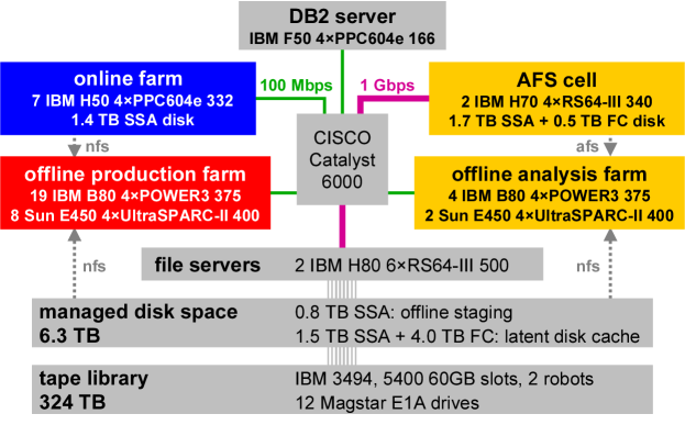
Figure 1: KLOE computing hardware configuration during 2001–2002.

The offline farm consists of a mix of IBM 7026-B80 SMPs running AIX, each with four 375-$\mathrm{MHz}$ Power3 CPUs; and Sun E450 SMPs running Solaris, each with four 400-$\mathrm{MHz}$ UltraSPARC II CPUs. In all, 23 B80s and 10 E450s are available, and provide a total processing power equivalent to about $110$ of the processors installed in the B80s, or about $30\,000$ SPECint2000.

The CPU time needed for data reconstruction and simulation is summarized in Table 1. Here and throughout this paper, all CPU times are referred to a single processor on one of the B80 servers. The CPU time needed for data reconstruction depends on the effectiveness of the filfo filter in rejecting background events in the presence of variable data-taking conditions. The entries in the table reflect the data-taking conditions in 2002, when filfo was able to reduce the input rate by 60%. Such events are rejected immediately after reconstuction in the EmC, which takes only 5 $\mathrm{ms}$. For events passing the filter, DC reconstruction takes about 40 $\mathrm{ms}$, where this number is a sample-weighted average of the reconstruction times for Bhabha events ($\sim$$30$ $\mathrm{ms}$), $\phi$-decay events ($\sim$$120$ $\mathrm{ms}$), and a small fraction of unrejected background events (15–40 $\mathrm{ms}$). Averaged over all input events, then, the time needed to reconstruct an event is 20 $\mathrm{ms}$.

Task	CPU time/event (ms)	CPU time/$\mathrm{fb}^{-1}$ (days)
Data reconstruction	20	9600
Data simulation ($\phi$ decays)	200	6650
Monte Carlo reconstruction	175	5100

Table 1: CPU-time consumption for reconstruction and Monte Carlo simulation on the KLOE offline farm. All CPU times refer to a single processor on one of the B80 servers.

Currently, about 80% of the processing power is used for production-related tasks; the remainder is allocated to physics analysis tasks. Additional machines can be opened to user batch and interactive sessions as the need arises. In this configuration, the total processing power allocated to production is adequate for the purposes of data reconstruction in parallel with acquisition. Fig. 2 illustrates the progress of the 2002 data-taking campaign. The growth of the reconstructed data set closely follows that of the acquired data set. From the point of view of both hardware and software, the operation of the offline systems is seen to be smooth and reliable.

Figure 2: a) Integrated luminosity per week in 2002. b) Total integrated luminosity vs. data-taking week in 2002. Histograms refer to the data taking; triangles refer to the reconstructed sample.

The time needed for DST production varies from stream to stream. This is in part because of the different abundances of selected events, and in part because the algorithms applied vary in CPU intensity (as noted in Sec. 3.1, $K^{+}$$K^{-}$ events are completely re-reconstructed at the DST production stage). DST-production rates range from $50~{}\mathrm{nb}^{-1}/\mbox{CPU~{}hour}$ for the $K^{+}$$K^{-}$ stream, to $600~{}\mathrm{nb}^{-1}/\mbox{CPU~{}hour}$ for the radiative $\phi$-decay stream. Processing of all four streams proceeds at $40~{}\mathrm{nb}^{-1}/\mbox{CPU~{}hour}$.

During the past three years of operation, the power of the offline farm has grown in parallel with the demands of the experiment, from 16 B80 CPU equivalents in the year 2000, to the 110 currently available. As part of an offline-system upgrade for the year 2004, ten new IBM p630 servers, each with four 1.45-$\mathrm{GHz}$ Power4+ processors, are currently being installed. This increases the total CPU power of the offline farm to about 225 B80 equivalents, or about $60\,000$ SPECint2000. The upgrade will provide CPU power sufficient for reconstruction, DST processing, and Monte Carlo production, simultaneously and in parallel with the acquisition of data at an average luminosity of $1\times 10^{32}$ $\mathrm{cm}^{-2}\,\mathrm{s}^{-1}$.

3.3 Data storage, data access, and networking

Data are permanently stored in an IBM 3494 tape library. The library has 12 Magstar 3590 tape drives which can read and write at 14 $\mathrm{MB}/\mathrm{s}$, dual active accessors, and space for about 5400 60-$\mathrm{GB}$ cartridges, for a maximum capacity of about 324 $\mathrm{TB}$. The library is maintained using IBM’s Tivoli Storage Manager [8]. The library usage is summarized in Table 2. Note that the specific volume of the raw data ($\mathrm{TB}/\mathrm{pb}^{-1}$) decreases from year to year because of background reduction due to better software filters and improved DAΦNE operations. During the running period scheduled for 2004, we expect that DAΦNE upgrades recently completed will allow us to collect a data set of about 2 $\mathrm{fb}^{-1}$. To store the new data, we will need at least an additional 300 $\mathrm{TB}$ of long-term storage capacity. To satisfy this need, we are currently in the process of ordering a second tape library.

Year	Int. Lum. ($\mathrm{pb}^{-1}$)	Raw (TB)	Recon. (TB)	MC (TB)	DST (TB)
2000	20	21	7	5	-
2001	180	47	18	7	3
2002	288	33	27	12	4
Total	488	101	52	24	7

Table 2: KLOE tape library usage at the end of 2002. The entries for DSTs include MC DSTs. DSTs were not produced for the 2000 data. A total of 184 $\mathrm{TB}$ are currently occupied.

A 6.3-$\mathrm{TB}$ offline-disk pool is used for data transfers to and from the library. The disk pool consists of 4.0 $\mathrm{TB}$ of Fibre Channel (FC) and 2.3 $\mathrm{TB}$ of SSA disks, configured in striping mode. Two IBM 7026-H80 SMPs running AIX, each with six 500-$\mathrm{MHz}$ RS64-III CPUs and 2 $\mathrm{GB}$ of RAM, locally mount the offline-disk pool and tape library and are used as file servers. With the two file servers working in concert, aggregate I/O rates of over 100 $\mathrm{MB}/\mathrm{s}$ have been obtained.

Analysis jobs usually use DSTs as input. For the 2001–2002 data, the set of DSTs occupies 4 $\mathrm{TB}$; MC DSTs occupy an additional 3 $\mathrm{TB}$. About 5.5 $\mathrm{TB}$ of the offline disk pool is used to cache files recalled from the tape library by the data-handling system; copies of the bulk of the DSTs reside in this cache for prompt access. The output from analysis jobs is written to user and working-group areas on the KLOE AFS cell. The AFS cell is served by two IBM 7026-H70 SMPs, each with four 340-$\mathrm{MHz}$ RS64-III CPUs, 850 $\mathrm{GB}$ of SSA disks, and 250 $\mathrm{GB}$ of FC disks, for a total cell capacity of 2.2 $\mathrm{TB}$. Users can access the AFS cell from PCs running Linux on their desktops to perform the final stages of their analyses.

Network connections are routed through a Cisco Catalyst 6000 switch. The file and AFS servers are connected to the switch via Gigabit Ethernet. Connections to all other nodes are via Fast Ethernet.

3.4 Data handling

A diagram of the data-handling scheme is presented in Fig. 3.

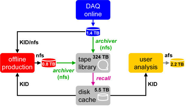
Figure 3: Schematic layout of KLOE data handling.

When new data are acquired, the online servers write the raw files to the online-disk pool. These files are then asynchronously archived to the tape library over an NFS mount by the archiver daemon. The archiving processes are tailored to minimize the number of tape mounts while guaranteeing enough space on the disk pool.

Normally, reconstruction is performed while the raw files are still resident on disk. For input to the reconstruction processes from the online disk, events are either read across an NFS mount or served by the data-handling system using a custom TCP/IP protocol, which is provided by the KLOE Integrated Dataflow package (kid) [9]. Reconstruction output is written via NFS to the offline-disk pool, from which it is asynchronously archived to tape. DSTs for each run are produced from the reconstruction output files, usually immediately after the run has been completely reconstructed. In this case, the reconstructed events may be read back in across the NFS mount for DST production. When files already archived and deleted from the online- or offline-disk pools must be processed on the offline farm, the recalld daemon restores the files from tape to the recall disk cache, from where they are served to the offline processes using the kid protocol. The spacekeeper daemon ensures the availability of disk space in the staging areas by deleting files that have been archived. The successful completion of calibration, reconstruction, and archival are signaled by flags in the database (see below).

The same model for data access used for reconstruction applies to user analysis jobs running on the offline farm. In principle, users may need to analyze raw, reconstructed, or DST files. If the files requested are resident on the online- or offline-disk pools, they are copied to the recall disk cache by recalld to be served to the user processes; otherwise, they are restored to the recall disk cache from tape. A filekeeper daemon ensures the availability of free space in the recall areas, deleting old files when necessary to make space for newly recalled data.

A central database based on IBM’s DB2 [10] is used to keep track of the locations of the several million files comprising the data set [11]. Each file is logged in the database when it is created. The database entry contains the reconstruction status of the file, allowing files that require processing to be easily identified. This database also contains run-by-run information on data-taking conditions and operational parameters of the detector, as noted in Sec. 3.1.

The backbone of the data-handling system is the kid package, which consists of two pieces: a centralized data-handling daemon, which coordinates the distributed file-moving services; and a client library, with an easy-to-use URL-based interface that allows access to files independent of their locations. kid URLs may incorporate SQL queries used to interrogate the file database. Examples of such URLs include:

• All raw files in the stated run range that have not yet been reconstructed:
  dbraw:run_nr between 23000 and 24000 and analyzed is not null

• All reconstructed files in the $K_{S}$$K_{L}$ stream for a given run:
  dbdatarec:run_nr = 23015 and stream_code = ksl

3.5 Software environment

The datarec program is built upon the framework provided by the analysis_control (a_c) package developed at FNAL [12]. a_c provides the tools for building the executable from KLOE analysis modules, as well as a user interface that allows the processing sequence and choice of enabled streams to be specified at run time. In order to use a_c in the KLOE environment, numerous customizations of the library have been implemented; in particular, the kid package (Sec. 3.4) has been seamlessly interfaced. The source code versions for analysis modules used in the datarec program are tracked using cvs [13].

The data format consists of independent collections of tabular data structures, or banks, for each event. They are read and written using the ybos package [14], which provides tools for platform-independent memory management and for the definition of tabular data structures that can be manipulated in Fortran code.

An interface to the zlib library [15] has also been added to a_c to allow reading and writing of compressed data. The compression/decompression routines are transparently called from a_c internals. A compression factor of about 0.6 is obtained for reconstructed output.

3.6 Analysis considerations

In addition to production jobs, user analysis jobs also run on the offline farm. In 2003, about 20% of the offline CPU power was avaliable to users for the production of histograms and Ntuples. About two-thirds of the machines open to user sessions were reserved for batch jobs, with queues managed by IBM’s LoadLeveler [16].

As an example of the execution time for user jobs, consider the analysis of the 2001–2002 $K_{S}$$K_{L}$ data set, which consists of $4.5\times 10^{8}$ events in 1.4 $\mathrm{TB}$ of DSTs, the majority of which are resident on disk in the recall disk cache for prompt access. With six batch jobs running in parallel (the default per-user maximum), the entire data set can be analyzed in six days elapsed. The output size ranges from 10 to 100 $\mathrm{GB}$, which can be accessed in situ on the AFS cell or copied off to a user’s desktop PC.

4 Reconstruction program and algorithms

4.1 Reconstruction algorithms for the drift chamber

The track-reconstruction algorithms [17] are based on the program developed for the ARGUS drift chamber [18]. This program has been adapted to the all-stereo geometry of the KLOE DC and tuned to the specific topology of KLOE events to optimize the efficiency of vertex reconstruction throughout the DC volume. The detailed DC geometry, the space-time ($s$–$t$) relations for the different types of drift cells, and the map of the magnetic field are described in detail in the database. Event reconstruction is performed in three steps: 1) pattern recognition, 2) track fitting, and 3) vertex fitting. Each step is handled separately and produces the input information for the subsequent step; this information is stored in ybos banks.

The first step of the track-reconstruction chain is pattern recognition (PR). The PR algorithm searches for track candidates and provides rough estimates of their parameters. Track segments are first searched for in the $xy$ plane; then the $z$ projections are obtained. In an axial drift chamber, the particle trajectory in the $xy$ plane is well approximated by a circle (except for corrections due to energy loss and multiple scattering, which are negligible at the PR stage). In the KLOE DC, since the wires are strung with a stereo angle, a particle leaves a pattern that appears as two nearby circles, one for each stereo view. The PR algorithm first searches for track candidates in each stereo view. Starting from the outermost layer, hit chains are built up by associating hits close in space on the basis of curvature compatibility. In order to resolve left-right ambiguities, a minimum of four hits in at least two wire layers are required to create a single-view track candidate.

At the end of the hit-association stage for each view, a filter exclusively assigns hits shared between track candidates to the better candidate. Each track candidate is then fitted and its parameters are computed. The track candidates from the two views are then combined in pairs according to their curvature values and geometrical compatibility. Finally, the $z$ projection for each pair is determined from a three-dimensional fit to all associated hits. At the PR stage, the magnetic field is assumed to be homogeneous, multiple scattering and energy loss are not treated, and rough $s$–$t$ relations (see Sec. 4.2) are used.

The track-fitting (TF) procedure minimizes a $\chi^{2}$ function based on the comparison between the measured and expected drift distances for each hit. Recurrent tracing relations are used at each step to determine the positions of successive hits from the estimated track parameters and the rough $s$–$t$ relations; the drift distance is then corrected using more refined $s$–$t$ relations that depend on the track parameters. Drift distances are recalculated with each iteration of the fit to make use of the previous determination of the track orientation with respect to the cell.

Tracks are described by connected helical segments. Local variations in the magnetic field are taken into account at each step, together with the effects of energy loss and multiple scattering. The momentum loss between consecutive hits is computed assuming the pion mass. Multiple scattering is accounted for by dividing the track into segments such that the estimated transverse displacement due to multiple scattering over the length of the segment is smaller than the spatial resolution. The values of the effective scattering angles in the transverse and longitudinal planes are then treated as additional parameters in the track fit.

After a first iteration, a number of procedures improve the quality of the track fit. In particular, dedicated algorithms are used to

• check the sign assignment of the drift distance hit by hit;

• add hits that were missed by the PR algorithm;

• reject hits wrongly associated to the track by the PR algorithm;

• identify split tracks and join them;

• identify kinked tracks and split them.

As an example of the performance of the TF procedure, in Fig. 4 we illustrate the momentum resolution for Bhabha events as a function of the polar angle $\theta$. Over a large range in $\theta$, $\sigma_{p}/p$ is $\sim$$0.3$%. The deterioration of the resolution at low angle is in accordance with the expected $\cot{\theta}$ behavior.

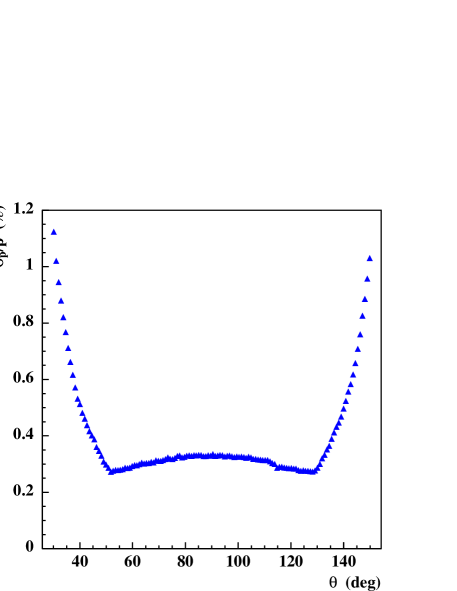
Figure 4: Momentum resolution $\sigma_{p}/p$ as a function of polar angle $\theta$, for Bhabha events.

At the end of the DC-reconstruction chain, the tracks from the TF procedure are used to search for primary and secondary vertices. For each track pair, a $\chi^{2}$ function is evaluated from the distances of closest approach between tracks; the covariance matrices from the TF stage are used to evaluate the errors. The vertex position is determined by minimizing this $\chi^{2}$. To reduce the number of combinations, the tracks are first extrapolated to the beam-crossing point in the transverse plane and primary vertices are searched for using tracks with an impact parameter smaller than 10% of their radius of curvature. Secondary vertices are then searched for among tracks not associated to any other vertex. For tracks that intersect the beam-pipe or inner DC walls, in the extrapolation, the track momentum is corrected for energy loss and the effect of multiple scattering is taken into account in the covariance matrix. The pion mass is assumed for the evaluation of these corrections.

For vertices inside the beam pipe, the vertex-position resolution is about 2 $\mathrm{mm}$ in $x$, $y$, and $z$. In Fig. 5, we show the distribution of the vertex-position residuals in $x$ for MC $K_{S}\to\pi^{+}\pi^{-}$ decays. The $\pi$$\pi$ invariant-mass distributions for $K_{S}\to\pi^{+}\pi^{-}$ decays in data and MC samples are compared in Fig. 6. The mass resolution for this decay is seen to be $\sim$$0.8$ MeV/$c^{2}$.

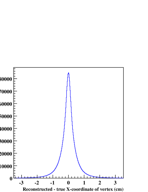
Figure 5: Distribution of vertex-position residuals in $x$ for MC $K_{S}\to\pi^{+}\pi^{-}$ events.

Figure 6: Invariant mass distributions for $K_{S}\to\pi^{+}\pi^{-}$ events. Points and histogram show the distributions for data and MC events, respectively.

Work is in progress on an algorithm to calculate the specific ionization $\d E/\d x$ for reconstructed tracks on the basis of the charge measurements from the ADCs recently added to the DC readout electronics.

4.2 Calibration of the space-time relations

Several effects influence the time response of the KLOE DC. The drift velocity of the helium-based gas mixture does not saturate with the electric field, so the relation between the drift time and the impact parameter of the track is not linear. Moreover, due to the geometry of the drift cells, the electric field configuration changes along the wire. This effect produces a dependence of the space-time ($s$–$t$) relations upon the orientation of the track and its position along the wire.

Simulations have shown that the $s$–$t$ relations can be parameterized in terms of the angles $\beta$ and $\tilde{\phi}$ defined in Fig. 7 [19]. Six cells with different values of $\beta$ have been chosen as reference cells. For each reference cell, the $s$–$t$ relations are parameterized for 36 bins in $\tilde{\phi}$, each 10^∘ wide. Since only the upper half of the cell is deformed, in 20 of the bins in $\tilde{\phi}$, the $s$–$t$ relations are the same for all six reference cells. There are therefore a total of $16\times 6+20=116$ parameterizations for the small cells, and 116 for the large cells. Each $s$–$t$ relation is represented as a 5^th-order Chebyshev polynomial [20], $t_{\mathrm{drift}}=P_{\mathrm{Cheb}}(C_{i}^{k},d)$, where $t_{\mathrm{drift}}$ is the measured time, $d$ is the impact parameter, and the $6\times 232$ coefficients $C_{i}^{k}$ ($k=1,\ldots,232$ and $i=0,\ldots,5)$ parameterize the “fine” $s$–$t$ relations as described above.

Figure 7: Definition of the angles $\beta$ and $\tilde{\phi}$.

The $s$–$t$ relations are determined using cosmic-ray events, which illuminate the chamber volume nearly uniformly and cover the entire range in the angle $\tilde{\phi}$. At the PR level, the values of $\tilde{\phi}$ and $\beta$ for each cell are unknown, since the trajectory of the particle has not yet been determined. At this level, the cell response is therefore described by a single $s$–$t$ relation, which is an average over all track orientations and drift-cell shapes. This “raw” $s$–$t$ relation is parameterized by the sum of three polynomials.

There are four contributions to the signal arrival time for each wire:

$$t=t_{\mathrm{TOF}}+t_{\mathrm{wire}}+t_{\mathrm{drift}}+t_{0}.$$ (1)

Here, $t_{\mathrm{TOF}}$ is the particle time of flight up to the wire hit, $t_{\mathrm{wire}}$ is the propagation time of the signal along the wire, $t_{\mathrm{drift}}$ is the drift time, and $t_{0}$ is a time offset. The offsets $t_{0}$ are calculated using cosmic-ray events at the beginning of each data-taking period (i.e., every few months), or whenever the readout electronics are reconfigured. About 10⁷ events are required in order to obtain the $t_{0}$ estimates. The $t_{\mathrm{drift}}+t_{0}$ terms are isolated by computing $t_{\mathrm{TOF}}$ and $t_{\mathrm{wire}}$ event-by-event, approximating cosmic-ray tracks by straight lines [6].

Calibration of the $s$–$t$ relations is performed by an iterative procedure which reconstructs tracks, checks the residuals (the difference between the impact parameters estimated using the existing $s$–$t$ relations and those given by the track fit), and, if required, produces a new set of calibration parameters. The procedure starts by reconstructing a calibration sample (typically, cosmic-ray events) with the standard PR and TF algorithms. The mean residuals as a function of reconstructed impact parameter are then obtained for each set of hits corresponding to each of the 232 $s$–$t$ relations. The impact parameters estimated from the drift time of each hit are then corrected by the corresponding value of the mean residual, and the tracks are reconstructed again. The iteration is halted when for each of the $232$ parameterizations, the corrections are smaller than 40 $\mu\mathrm{m}$ for hits in the central part of the drift region of their cells. Finally, the 232 fine $s$–$t$ relations are fitted, and the new coefficients $C^{k}_{i}$ are calculated.

The calibration program is incorporated into the KLOE online system. A synchronous procedure automatically starts at the beginning of each run, and selects $80\,000$ cosmic-ray events from the event-building nodes using kid. These events are then tracked using the existing $s$–$t$ relations, and the absolute value of the average of the residuals for hits in the central part of the drift region is monitored. If this value exceeds 40 $\mu\mathrm{m}$, $300\,000$ cosmic-ray events are collected, and the asynchronous procedure described above produces a new set of calibration constants. Depending on background conditions, the filters on the farm select events at a rate between 25 and 30 $\mathrm{Hz}$. The event collection therefore takes therefore about 3 hours, and a comparable amount of time is needed for the analysis [6]. A complete recalibration is only necessary a few times per data-taking period, essentially when the atmospheric pressure changes by more than 1%.

Fig. 8 shows the resolution averaged over all wires as a function of the reconstructed impact parameter. The spatial resolution is better than 200 $\mu\mathrm{m}$ over a large part of the drift cell.

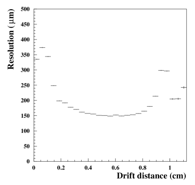
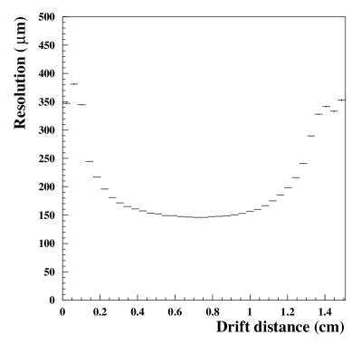
Figure 8: Spatial resolution as a function of the impact parameter for small (left) and large (right) cells.

4.3 Momentum calibration

The calibration of the absolute momentum scale was performed with the 2.4 $\mathrm{pb}^{-1}$ data sample collected in 2000 [21], in parallel with a survey of the mechanical distortions of the chamber and calibration of the space-time relations. Two- and three-body processes such as $e^{+}e^{-}\to e^{+}e^{-}$, $e^{+}e^{-}\to\mu^{+}\mu^{-}$, $e^{+}e^{-}\to\pi^{+}\pi^{-}\pi^{0}$, $K_{S}\to\pi^{+}\pi^{-}$, $K_{L}\to\pi^{+}\pi^{-}$, $K_{L}\to\pi\ell\nu$, $K_{L}\to\pi^{+}\pi^{-}\pi^{0}$, $K^{\pm}\to\pi^{\pm}\pi^{0}$, and $K^{\pm}\to\mu^{\pm}\nu$ were employed. Depending on the process, the invariant mass, missing mass, or secondary momentum in the rest frame of the decaying particle was reconstructed; deviations from the nominal values of these quantities were used as benchmarks for the calibration procedure. This approach allowed the investigation of distortion effects over the entire volume of the detector and the full range of momentum. Initially, the reconstructed momenta of low-angle Bhabha electrons deviated from the expected values by as much as 8 MeV/$c$. In general, the deviations showed a complex dependence on momentum, polar angle, azimuthal angle, and production point of the tracked particle.

Two main sources of distortions were identified:

1. Measurement artifacts in the magnetic-field map
   The magnetic field was mapped with a mechanical system for the positioning of an array of Hall probes at nominal field values of 0.3, 0.45, and 0.6 $\mathrm{T}$ before the DC was inserted into the solenoid [22]. In 2001, the maps were reexamined, with extra terms introduced to account for distortions due both to misalignment of the Hall probes with respect to their nominal positions on the arm spanning the solenoid volume, and to rotations and translations of the arm with respect to its nominal position in the KLOE reference system. Most of these geometrical effects could be isolated because the measurements were performed twice: first with the measurement arm moving from one end of the solenoid to the other, and then in the opposite direction, with the orientation of the measuring device reversed. Artifact field components thus appeared in the sum or difference of measurements performed by the same probe or by two neighboring probes. The typical size of artifact field components in the transverse plane was about 0.004 $\mathrm{T}$.

2. Saturation of the magnetic field
   For optimum DAΦNE performance, KLOE must work at a nominal field value of about 0.52 $\mathrm{T}$. A comparison of the maps at the three different nominal field values showed evidence for saturation. The effect was also found in a set of very precise measurements of the field as a function of current performed on the solenoid axis using an NMR probe. The NMR data showed deviations from linearity as large as 1%, increasing with distance from the solenoid axis and decreasing with distance from the endplates. Global corrections for the saturation of the longitudinal field component were applied using the shape of the excitation curve obtained by the NMR probe; local corrections were applied by interpolation of the three maps. Unfortunately, global saturation corrections for the transverse field components could not be computed. These corrections are thought to be on the order of 0.001 $\mathrm{T}$ in magnitude.

With these corrections, low-angle Bhabha electrons are reconstructed with systematic momentum deviations of less then 500 keV/$c$, or approximately 0.1%. Similar accuracy is found for all benchmark modes. The residual systematic differences can be ascribed to interpolation error in the saturation correction.

4.4 Reconstruction algorithms for the calorimeter

The calorimeter is segmented into 2440 cells, which are read out by PMTs at each end (referred to as sides $A$ and $B$ in the following). Both charges $Q_{\mathrm{ADC}}^{A,B}$ and times $t_{\mathrm{TDC}}^{A,B}$ are recorded. For each cell, the particle arrival time $t$ and the impact point $s$ along the fiber direction are reconstructed using the times at the two ends as

$$\begin{array}[]{l}t={1\over 2}(t^{A}+t^{B}-t_{0}^{A}-t_{0}^{B})-\frac{L}{2v},\\ s={v\over 2}(t^{A}-t^{B}-t_{0}^{A}+t_{0}^{B}),\end{array}$$ (2)

with $t^{A,B}=c^{A,B}\,t_{\mathrm{TDC}}^{A,B}$, where $c^{A,B}$ are the TDC calibration constants, $t_{0}^{A,B}$ are the overall time offsets, and $L$ and $v$ are the cell length and the light velocity in the fibers. The impact position in the transverse direction is provided by the locations of the readout elements.

The energy signal $E_{i}$ on each side of cell $i$ is determined as

$$E_{i}=\kappa_{E}\,g_{i}(s){S_{i}\over S_{\mathrm{mip},\,i}},$$ (3)

where $S=Q_{\mathrm{ADC}}-Q_{0,\,\mathrm{ADC}}$ is the charge collected after subtraction of the zero-offsets, and $S_{\mathrm{mip}}$ is the response to a minimum-ionizing particle crossing the calorimeter center. The correction factor $g(s)$ accounts for light attenuation as a function of the impact position $s$ along the fiber, while $\kappa_{E}$ is the overall energy scale factor. The final value of $E_{i}$ for the cell is taken as the mean of the determinations at each end.

The calibration constants related to minimum-ionizing particles, $S_{\mathrm{mip}}$ and $g$, are acquired with a dedicated trigger before the start of each long data-taking period. The time offsets $t_{0}^{A,B}$ and the light velocity $v$ in the fibers are evaluated every few days using high-momentum cosmic rays selected using drift-chamber information. In this iterative procedure, the tracks reconstructed in the drift chamber are extrapolated through the calorimeter, and the residuals between the expected and measured times for each cell are minimized. Finally, a procedure to determine the value of $\kappa_{E}$ and to refine the values of $t_{0}^{A,B}$ runs online [5]; it uses Bhabha and $e^{+}e^{-}\to\gamma\gamma$ events to establish a new set of constants each 100–200 $\mathrm{nb}^{-1}$ (i.e., approximately every 2 hours during normal data taking). The procedures used to calibrate the calorimeter are further discussed in Ref. 2.

Calorimeter reconstruction starts by applying the calibration constants to convert the measured quantities $Q_{\mathrm{ADC}}$ and $t_{\mathrm{TDC}}$ to the physical quantities $S$ and $t$. Position reconstruction and energy/time corrections vs. $s$ are then performed for each fired cell. Next, a clustering algorithm searches for groups of cells belonging to a given particle. In the first step, cells contiguous in $r\phi$ or $xz$ are grouped into pre-clusters. In the second step, the longitudinal coordinates and arrival times of the pre-clusters are used for further merging and/or splitting. The cluster energy, $E_{\mathrm{cl}}$, is the sum of the energies for all cells assigned to a cluster. The cluster position, $(x,y,z)_{\mathrm{cl}}$, and time, $t_{\mathrm{cl}}$, are computed as energy-weighted averages over the contributing cells. Cells are included in the cluster search only if times and amplitudes are available on both sides; otherwise, they are listed as “incomplete” cells. The available information from most of the incomplete cells is added to the existing clusters at a later stage by comparison of the $(x,y)$ positions of such cells with the cluster centroids.

The production of fragments from electromagnetic showers has been studied by comparing data and Monte Carlo samples of $e^{+}e^{-}\to\gamma\gamma$ events, with tight selection cuts applied to the two highest-energy clusters in the event (the “golden photons”). The distribution of the minimum distance $|\Delta\mathbf{x}|$ between the golden photons and any of the other clusters is characterized by reasonable agreement between data and MC at large values of $|\Delta\mathbf{x}|$; at low values of $|\Delta\mathbf{x}|$ an appreciable discrepancy is observed. In this latter case, a similar discrepancy is observed for the distribution of the difference in time, $\Delta t$, between the selected clusters. The multiplicity of fragments in data exceeds that in MC events by about a factor of two and is dominated by clusters with energy below 50 MeV. We attribute these discrepancies to small inaccuracies in the descriptions of the shower development and time response in the Monte Carlo, so that the longitudinal cluster-breaking procedure performs differently for data and MC events. For this reason, depending upon the multiplicity of photons in the event, a split-cluster recovery procedure is applied at the analysis level to merge close clusters depending on their values of $|\Delta\mathbf{x}|$, $\Delta t$, and energy.

The energy, timing, and position resolutions for photons are measured using $e^{+}e^{-}\to\pi^{+}\pi^{-}\pi^{0}$ and radiative Bhabha samples. In both cases, the energy $E_{\gamma}$ and direction $\mathbf{\hat{p}}_{\gamma}$ of one of the photons are predicted with high precision using only tracking information. The calorimeter response and resolution as a function of the photon polar angle $\theta_{\gamma}$ and energy $E_{\gamma}$ can therefore be parameterized, and the photon detection efficiency can be measured with high accuracy.

The energy response as a function of $E_{\gamma}$ shows a linearity better than 1% down to 60 MeV, while a drop in the response of $\sim$$3$% is observed at low energy. This is mostly due to imperfect recovery of the “incomplete” cells. The energy resolution is dominated by sampling fluctuations and is well parameterized as $5.7\%/\surd E(\mbox{GeV})$. The light yield has been estimated by looking at the fluctuations in the ratio of the energy response at each side, $E^{A}/E^{B}$, and corresponds to $\sim$$700$ photoelectrons per side for 1 GeV photons impinging at the center of the calorimeter [$\sigma_{E}/E,\mbox{p.e. stat.}\approx 2.7\%/\surd E(\mbox{GeV})$]. The timing resolution has also been determined; the stochastic term is dominated by the light yield, and scales as $54~{}\mathrm{ps}/\surd E(\mbox{GeV})$, while a constant term of 140 $\mathrm{ps}$ must be added in quadrature to account for the jitter introduced by rephasing the KLOE trigger with the machine RF. The contribution due to the precision of the channel-by-channel calibration is estimated to be $\sim$$50$ $\mathrm{ps}$. In the transverse coordinates, the position resolution is dominated by the readout granularity, and is $\mbox{$\sim$$4.4$}/\surd 12$ $\mathrm{cm}$, while in the longitudinal coordinate, $s$, it shows the expected $1.2~{}\mathrm{cm}/\surd E(\mbox{GeV})$ energy dependence. The reconstruction of the masses of neutral mesons ($\pi^{0}$, $\eta$, $K_{S}$, $K_{L}$) decaying to $n$-photon final states shows that, at KLOE energies, the mass resolution is completely dominated by the energy resolution, while the mass scale is set with an accuracy better than 1%. In Fig. 9, we compare the distributions of reconstructed $\pi^{0}$ and $K_{S}$ masses for $K_{S}\to\pi^{0}\pi^{0}$ events from data and MC.

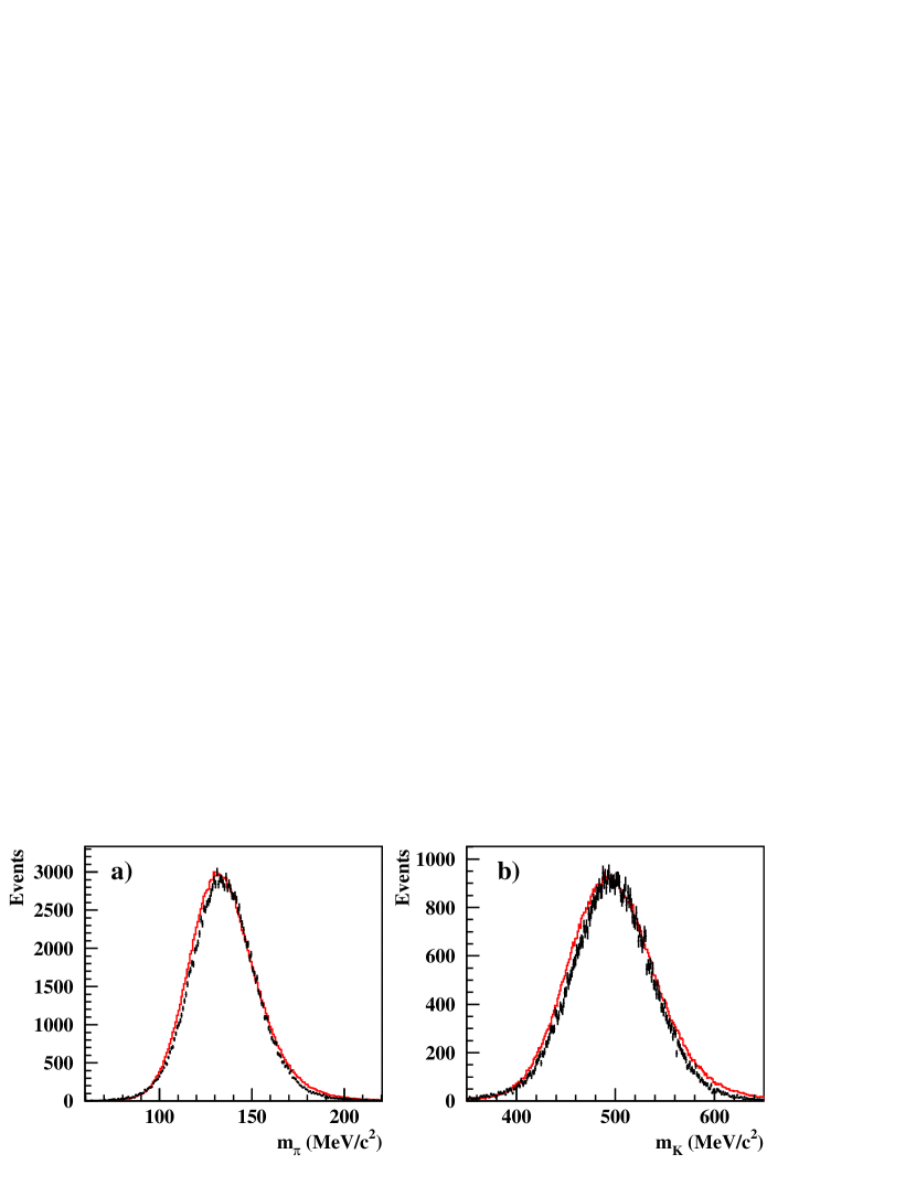
Figure 9: Reconstructed invariant-mass distributions for a) $\pi^{0}$’s and b) $K_{S}$’s from $K_{S}\to\pi^{0}\pi^{0}$ events. Points are for data; solid line is for MC.

4.5 Determination of the absolute time scale and event-start time

To run at the design luminosity, DAΦNE can operate with 120 bunches per ring, which corresponds to a bunch-crossing period equal to the machine RF period, $t_{\mathrm{RF}}=2.715$ $\mathrm{ns}$. Due to the large spread of the particle arrival times and short bunch-crossing period, the trigger time does not identify the bunch crossing that produced an event; the time at which this bunch crossing occurred must therefore be determined offline. In order not to spoil the excellent EmC time resolution, the start to the TDC system is obtained by synchronizing the level-1 trigger with a clock that is phase-locked to the DAΦNE radiofrequency signal. The clock period is $4t_{\mathrm{RF}}=10.85~{}\mathrm{ns}$. The calorimeter times are measured in common-start mode and are given by the TDC stops from the discriminated PMT signals:

$$t_{\mathrm{cl}}=t_{\mathrm{TOF}}+\delta_{\mathrm{c}}-N_{\mathrm{BC}}\,t_{\mathrm{RF}},$$ (4)

where $t_{\mathrm{TOF}}$ is the time of flight of the particle from the event origin to the calorimeter, $\delta_{\mathrm{c}}$ is the sum of all offsets due to electronics and cable delays, and $N_{\mathrm{BC}}\,t_{\mathrm{RF}}$ is the time needed to generate the TDC start (see Fig. 10).

The quantities $\delta_{\mathrm{c}}$ and $t_{\mathrm{RF}}$ are determined using $e^{+}e^{-}\to\gamma\gamma$ events. For such events, the distribution of $\Delta_{\mathrm{TOF}}=t_{\mathrm{cl}}-r_{\mathrm{cl}}/c$ shows well-separated peaks corresponding to the different values of $N_{\mathrm{BC}}$ for events in the sample (see Fig. 11a). We define $\delta_{\mathrm{c}}$ as the position of the largest peak in the distribution, and obtain $t_{\mathrm{RF}}$ from the distance between peaks. This is done by calculating the discrete Fourier transform of the $\Delta_{\mathrm{TOF}}$ distribution and fitting the peak around $\nu=1/t_{\mathrm{RF}}$ (see Fig. 11b). The absolute TDC time scale is obtained by imposing $t_{\mathrm{RF}}(\mathrm{fit})=t_{\mathrm{RF}}$. Both $\delta_{\mathrm{c}}$ and $t_{\mathrm{RF}}$ are determined with precision better than 4 $\mathrm{ps}$ for every 200 $\mathrm{nb}^{-1}$ accumulated.

Figure 10: Timing scheme for bunch-crossing signal, calorimeter signals, and level-1 trigger formation.

Figure 11: Calibration of EmC time scale using $e^{+}e^{-}\to\gamma\gamma$ events: a) Distribution of $\Delta_{\mathrm{TOF}}$, b) Detail of the peak at $\nu=1/t_{\mathrm{RF}}$ in the discrete Fourier transform of the $\Delta_{\mathrm{TOF}}$ distribution, c) $\Delta_{\mathrm{TOF}}$ as a function of $z_{\mathrm{cl}}$, d) $\Delta_{\mathrm{TOF}}$ as a function of $z_{\mathrm{cl}}$ for a single peak in the $\Delta_{\mathrm{TOF}}$ distribution, corresponding to a single value of $N_{\mathrm{BC}}$.

While measuring the ratio $\mathrm{BR}(K_{S}\to\pi^{+}\pi^{-})$/$\mathrm{BR}(K_{S}\to\pi^{0}\pi^{0})$, we found it necessary to apply an absolute correction of $\sim$$0.8$% to the time scale to eliminate an observed dependence of $\beta^{*}_{K}$ on the trigger-formation time [23, 24]. The error on the time scale was found to originate from two cooperating effects:

• As seen from the distribution of $\Delta_{\mathrm{TOF}}$ as a function of $z_{\mathrm{cl}}$ in Fig. 11c, the characteristic value of $N_{\mathrm{BC}}$ in $e^{+}e^{-}\to\gamma\gamma$ events varies as a function of longitudinal position along the barrel. This is due to the light-propagation time in the fibers, which is the dominant delay in trigger-signal formation.

• Because of a residual slewing effect, for any given value of $N_{\mathrm{BC}}$, $\Delta_{\mathrm{TOF}}$ depends on $z_{\mathrm{cl}}$, as seen from Fig. 11d.

When taken together, these two effects lead to an error in determining the distance between the peaks in the $\Delta_{\mathrm{TOF}}$ distribution. Since 2001, we have corrected for the dependence of $\Delta_{\mathrm{TOF}}$ on $z_{\mathrm{cl}}$ using an ad hoc procedure before calibrating the calorimeter. This provides a stable $-0.7\%$ correction to the time scale.

Since we want the cluster times to correspond to particle times of flight, a time offset $t_{0,\,\mathrm{evt}}\equiv\delta_{\mathrm{c}}-N_{\mathrm{BC}}\,t_{\mathrm{RF}}$ must be subtracted from all cluster times (see Eq. [4]). The trigger-formation time $N_{\mathrm{BC}}\,t_{\mathrm{RF}}$ varies on an event-by-event basis; it is determined offline at different points of the reconstruction path. A zeroth-order value for $N_{\mathrm{BC}}$ (and hence $t_{0,\,\mathrm{evt}}$) is obtained by assuming that the earliest cluster in the event is due to a prompt photon from the interaction point. By imposing $t_{\mathrm{TOF}}=r_{\mathrm{cl}}/c$ for this cluster, we obtain

$$t_{0,\,\mathrm{evt}}=\delta_{\mathrm{c}}-\mbox{Nint}\!\left[\frac{r_{\mathrm{cl}}/c-t_{\mathrm{cl}}+\delta_{\mathrm{c}}}{t_{\mathrm{RF}}}\right]t_{\mathrm{RF}},$$ (5)

where $\mbox{Nint}[\,]$ stands for the nearest integer to the quantity in brackets. We refer to $t_{0,\,\mathrm{evt}}$ as the event-start time.

Soft clusters coming from the accidental coincidence of machine-background events with the $e^{+}$$e^{-}$ collision can arrive earlier than the fastest cluster from the collision event itself. To increase the reliability of the estimate of $t_{0,\,\mathrm{evt}}$, the cluster used for its evaluation must also satisfy the conditions $E_{\mathrm{cl}}>50$ MeV and $(x_{\mathrm{cl}}^{2}+y_{\mathrm{cl}}^{2})^{1/2}>60$ $\mathrm{cm}$.

4.6 Track-to-cluster association

The track-to-cluster association module establishes correspondences between tracks in the drift chamber and clusters in the calorimeter.

The procedure starts by assembling the reconstructed tracks and vertices into decay chains and isolating the tracks at the ends of these chains. For each of these tracks, the measured momentum and the position of the last hit in the drift chamber are used to extrapolate the track to the calorimeter. The extrapolation gives the track length $L_{\mathrm{ex}}$ from the last hit in the chamber to the calorimeter surface, and the momentum $\mathbf{p}_{\mathrm{ex}}$ and position $\mathbf{x}_{\mathrm{ex}}$ of the particle at the surface. The resulting impact point is then compared with the positions $\mathbf{x}_{\mathrm{cl}}$ of the reconstructed cluster centroids. A track is associated to a cluster if the distance to the centroid in the plane orthogonal to the direction of incidence of the particle on the calorimeter, $D_{\mathrm{tcl}}=\left|(\mathbf{x}_{\mathrm{cl}}-\mathbf{x}_{\mathrm{ex}})\,\mbox{\boldmath{$\times$}}\,\mathbf{p}_{\mathrm{ex}}/\!\left|\mathbf{p}_{\mathrm{ex}}\right|\right|$, is less than 30 $\mathrm{cm}$. For each track, the associated clusters are ordered by ascending $D_{\mathrm{tcl}}$ values.

Various event-classification algorithms classify clusters as due to neutral or charged particles. Most of these algorithms treat clusters as due to neutral particles if no associated tracks are identified by the track-to-cluster association module.

While the standard track-to-cluster association algorithm provides the information necessary to estimate the arrival time for a charged particle at the surface of the calorimeter, the interval between the time of particle incidence and the measured cluster-centroid time, $\Delta t_{\mathrm{EmC}}$, can be significant, and must be taken into consideration in time-of-flight based particle-identification schemes. For example, for $\pi^{+}$’s which interact deeply (25–30 $\mathrm{cm}$) in the calorimeter, $\Delta t_{\mathrm{EmC}}$ can be as much as 1 $\mathrm{ns}$, as compared to a time of flight of $\sim$$8$ $\mathrm{ns}$. This time interval directly reflects the temporal profile of the energy deposition for the incident particle, and varies by particle species. For each species ($e^{+}$, $e^{-}$, $\mu^{+}$, $\mu^{-}$, $\pi^{+}$, and $\pi^{-}$), a simple, linear parameterization can be used to relate $\left<\Delta t_{\mathrm{EmC}}\right>$ to the depth of the centroid along the direction of particle incidence. Because of residual differences between the temporal shower profiles observed in data and simulated in the Monte Carlo, these parameterizations have been performed separately using data and MC events. They are available for use in calculating expected particle times of flight at the analysis level.

4.7 Event classification

The KLOE event-classification library is composed of different modules for the identification of the major physics channels at DAΦNE. The main classification algorithms include those for the identification of

• generic background: beam background, cosmic-ray muons, and fragments of small-angle Bhabhas;

• large-angle Bhabhas and $e^{+}e^{-}\to\gamma\gamma$ events;

• tagged $K_{L}$ or $K_{S}$ decays;

• tagged $K^{+}$ or $K^{-}$ decays;

• $\phi\to\pi^{+}\pi^{-}\pi^{0}$ decays;

• $\pi^{+}\pi^{-}+n\gamma$ and fully neutral $n\gamma$ final states coming from various primary processes such as $e^{+}e^{-}\to\pi^{+}\pi^{-}\gamma$, $e^{+}e^{-}\to\phi\to\eta\gamma$ or $\eta^{\prime}\gamma$, $e^{+}e^{-}\to\phi\to f_{0}(980)\gamma$ or $a_{0}(980)\gamma$, etc.

Background events are discarded, while all of the other samples are separately archived (see also Sec. 3.1). In the following, we discuss the criteria used to identify events in each of these categories.

The background-rejection algorithm is based on calorimeter clustering and DC hit counting, so that background events can be eliminated before DC reconstruction, which is the most CPU-intensive section of our reconstruction program. For the identification of background events, cuts are applied on the number of clusters; the number of DC hits; the total energy in the calorimeter; the average polar angle, position, and depth of the (two) most energetic cluster(s); and the ratio between the number of hits in the innermost DC layers and the total number of DC hits. These cuts have been studied to minimize losses for physics channels. Additionally, a simple cut on anomalously high total energy deposits in the calorimeter is included to reject rarer machine-background topologies due to sporadic DAΦNE beam-loss events.

The KLOE trigger system includes a veto for cosmic-ray muons that uses dedicated thresholds on the energy deposition in the outermost layer of the calorimeter. Cosmic-ray events that survive the trigger veto ($\sim$$0.6$ $\mathrm{kHz}$ out of $\sim$$3$ $\mathrm{kHz}$) are rejected by the background filter by identification of at least one cluster pair with relative timing, total energy deposition, and energy released in the outermost calorimeter layer consistent with those expected for a relativistic muon.

Small-angle Bhabha electrons can strike the focusing quadrupoles and shower inside the magnets and/or the QCAL calorimeter. Fragments from these showers are sometimes sufficient to trigger the experiment. Events of this type are identified by the presence of spatially concentrated clusters on the endcap calorimeters that arrive within a narrow time window.

Large-angle Bhabha and $e^{+}e^{-}\to\gamma\gamma$ events are selected to calibrate the calorimeter and to evaluate the luminosity. These events are identified using only calorimetric information. They must have at least two clusters with energy $300~{}\mbox{MeV}<E_{\mathrm{cl}}<800~{}\mbox{MeV}$ and polar angle between $45^{\circ}<\theta<135^{\circ}$. These clusters must arrive within a narrow time window and have $|180^{\circ}-\theta_{1}-\theta_{2}|<10^{\circ}$. A stringent cut on the angle between the two most energetic clusters, $\mathbf{x}_{1}\mbox{\boldmath{$\cdot$}}\mathbf{x}_{2}/\!\left|\mathbf{x}_{1}\right|\!\left|\mathbf{x}_{2}\right|<-0.975$, is used to separate $\gamma\gamma$ events from Bhabhas.

A more precise measurement of the integrated luminosity is obtained by refining the large-angle Bhabha event selection with track reconstruction information. In particular, the two tracks in the event with the greatest number of associated DC hits must be of opposite charge and have momenta $p>400~{}\mbox{MeV}/c$ and polar angles $55^{\circ}<\theta<125^{\circ}$. The agreement obtained for the distributions of important quantities such as the energy and angle of the Bhabha clusters for data and Monte Carlo events (generated with babayaga [25, 26]) demonstrates that the event counting in the fiducial angular region is accurate to the same level as the precision of the generator itself.

At KLOE, it is possible to tag $K_{S}$, $K_{L}$, $K^{+}$, and $K^{-}$ beams: the presence of a $K_{S}$ ($K_{L}$) signals the presence of a $K_{L}$ ($K_{S}$) on the opposite side of the detector, and the same applies for $K^{+}$’s and $K^{-}$’s. Pure $K_{L}$ beams are tagged by the identification of the $K_{S}\to\pi^{+}\pi^{-}$ decay. One charged vertex from two particles originating near the interaction point (IP) is required. Loose cuts on vertex position, particle momenta, and invariant mass are applied. The reconstruction of the $K_{S}$ decay allows the $K_{L}$ momentum to be predicted with a precision of better than 2 MeV/$c$. The overall tagging efficiency is $\sim$$70$%. $K_{S}$ beams are tagged by $K_{L}$ interactions in the calorimeter barrel. These interactions are signaled by high-energy clusters with typical arrival times of 30 $\mathrm{ns}$ due to the low momentum (110 MeV/$c$) of the kaons produced at DAΦNE. $K_{L}$ clusters used to tag $K_{S}$’s must have energy $E_{\mathrm{cl}}>100$ MeV and velocity $0.17<\beta<0.28$, and must not be associated to any tracks in the drift chamber. The $K_{S}$ momentum is determined with a precision of better than 2 MeV/$c$, as is also the case for the $K_{L}$ beam. A $K_{S}$ beam can also be tagged by looking for $K_{L}\to\pi^{+}\pi^{-}\pi^{0}$ decays, which are identified by the presence of a vertex in the DC satisfying kinematic cuts, and two clusters from the $\pi^{0}\to\gamma\gamma$ decay. These clusters must satisfy opening-angle and time-of-flight cuts and must not be associated to any tracks in the DC.

At KLOE, since the $K_{S}$$K_{L}$ pairs from $\phi$ decay are initially in a pure, antisymmetric state, the final-state decay products show characteristic interference patterns. By studying the relative-time distributions for decays to different final states, it is possible to measure various $CP$- and $CPT$-violation parameters [27]. The most interesting events for this type of analysis are those in which the $K_{S}$ and $K_{L}$ decays occur in close proximity to each other, i.e., both occur near the IP. In order to maximize the selection efficiency for such topologies, a dedicated algorithm has been developed. This algorithm searches for the presence of any combination of pairs of track and photon vertices that represent a possible pair of $K_{S}$ and $K_{L}$ decay modes. Good track vertices must have exactly two tracks of opposite charge.

Events are selected for the charged-kaon sample by the identification of either a pair of candidate kaon tracks originating near the IP, or a $K\to\mu\nu$ or $K\to\pi\pi^{0}$ decay in the DC. In the first case, two tracks of opposite charge with total momentum compatible with the $\phi$ decay kinematics are required. In the second case, the kaon decay is recognized as a charged vertex with two connected tracks of the same sign of charge. The vertex must lie within $40<R_{xy}<150$ $\mathrm{cm}$, and the momentum of the secondary in the rest frame of the kaon must be within the range $180<p^{*}<270$ MeV/$c$.

The $\phi\to\pi^{+}\pi^{-}\pi^{0}$ sample is obtained by searching for a vertex near the IP ($R_{xy}<8$ $\mathrm{cm}$, $\left|z\right|<15$ $\mathrm{cm}$) with two connected tracks of opposite charge. Cuts on the sum of the track momenta, $p_{\mathrm{sum}}=\left|\mathbf{p}_{1}\right|+\left|\mathbf{p}_{2}\right|$, the missing momentum, $p_{\mathrm{miss}}$, and the missing energy, $E_{\mathrm{miss}}$, are used to isolate the sample (see Fig. 12).

Figure 12: Distribution of $\left|\mathbf{p}_{1}\right|+\left|\mathbf{p}_{2}\right|$ vs. $cp_{\mathrm{miss}}-E_{\mathrm{miss}}$. a) $\phi\to\pi^{+}\pi^{-}\pi^{0}$ decays are in the bottom-left region of the plot, while $\pi^{+}\pi^{-}(\gamma)$, $\mu^{+}\mu^{-}(\gamma)$, and $e^{+}e^{-}(\gamma)$ events are concentrated in the top-right region. b) Enlarged view of the top-right region, showing the contributions from $\pi^{+}\pi^{-}(\gamma)$, $\mu^{+}\mu^{-}(\gamma)$, and $e^{+}e^{-}(\gamma)$ events.

The search for the final states $(\pi^{+}\pi^{-},\ \mu^{+}\mu^{-},\ e^{+}e^{-})+n\gamma$ requires one charged vertex near the IP with $p_{\mathrm{sum}}<1020$ MeV/$c$, $m_{\pi\pi}>90$ MeV, and $cp_{\mathrm{miss}}-E_{\mathrm{miss}}>-50$ MeV. Different windows in $p_{\mathrm{sum}}$ and the quantity $cp_{\mathrm{miss}}-E_{\mathrm{miss}}$ are used to separate $\pi/\mu/e$ final states, as seen in Fig. 12.

Fully neutral $n\gamma$ final states are identified by the presence of at least three clusters in the calorimeter that are not associated to tracks in the DC, and which have times of flight consistent with photon travel from the IP.

4.8 Redetermination of the event-start time

As explained in Sec. 4.5, the event-start time $t_{0,\,\mathrm{evt}}$, or equivalently, the integer number of bunch crossings $N_{\mathrm{BC}}$ needed for trigger formation, must be determined offline by analysis of the cluster times. Before tracking and event classification, $N_{\mathrm{BC}}$ is obtained by assuming that the earliest qualifying cluster in the event is due to a photon coming from the IP. This first determination allows the event to be reconstructed and classified by physics channel. However, many physics channels contain no prompt photons in the final state, so this determination of $N_{\mathrm{BC}}$, and therefore, the corrected cluster times $t_{\mathrm{cl}}^{(0)}$, may differ from the actual times of flight by an integer number of bunch crossings $\Delta N_{\mathrm{BC}}$:

$$t_{\mathrm{cl}}^{(0)}=t_{\mathrm{TOF}}-\Delta N_{\mathrm{BC}}\,t_{\mathrm{RF}}.$$ (6)

For such events, it is usually possible to obtain the remaining correction term using a recognized topology associated to a cluster. The term needed is then

$$\Delta N_{\mathrm{BC}}\,t_{\mathrm{RF}}=\frac{L}{\beta c}-t_{\mathrm{cl}}^{(0)},$$ (7)

where $L$ is the estimated path length from the origin to the selected cluster, and $\beta$ is evaluated using the relevant mass hypothesis. For example, if $\Delta N_{\mathrm{BC}}$ is evaluated from a primary track, $\beta$ is evaluated from the track momentum. If the track associated to the cluster comes from a secondary vertex, the term $L/\beta c$ becomes $\sum_{i}L_{i}/\beta_{i}c$, where the sum is over the contributions from primary and secondary particles (including possibly photons). The times of all clusters in the event are then reevaluated as $t_{\mathrm{cl}}=t_{\mathrm{cl}}^{(0)}+\Delta N_{\mathrm{BC}}\,t_{\mathrm{RF}}$. This procedure has been implemented for events classified as

• charged kaons, by the identification of a $K\to\pi\pi^{0}$ or $K\to\mu\nu$ decay;

• neutral kaons, by the identification of a $K_{S}\to\pi^{+}\pi^{-}$ decay;

• neutral radiative decays.

For charged-kaon events, if the $K\to\pi\pi^{0}$ topology is recognized, the extrapolations to the calorimeter of the clusters from the $\pi^{0}\to\gamma\gamma$ decay and the charged-pion track can be used to determine $\Delta N_{\mathrm{BC}}$. If instead the $K\to\mu\nu$ topology is recognized, $\Delta N_{\mathrm{BC}}$ is estimated from the momenta and lengths of the kaon and muon tracks. For neutral-kaon events with $K_{S}\to\pi^{+}\pi^{-}$ decays, $\Delta N_{\mathrm{BC}}$ is determined using the first pion to reach the calorimeter. Neutral radiative decays do contain prompt photons; the goal in redetermining the event-start time in this case is to correct situations in which $N_{\mathrm{BC}}$ is at first incorrectly determined because of the accidental coincidence of (a) beam-background cluster(s). For such events, if the second cluster with $E_{\mathrm{cl}}>50$ MeV and $R_{xy}>60$ $\mathrm{cm}$ arrives more than 4 $\mathrm{ns}$ after the first, $\Delta N_{\mathrm{BC}}$ is calculated using the second cluster.

4.9 Reconstruction of photon vertices in $K_{L}$ decays

The positions of photon vertices from $K_{L}$ decays are obtained from the cluster times. Each photon defines a time-of-flight triangle: the first side is the segment from the IP to the $K_{L}$ decay vertex, $\mathbf{L}_{K}$; the second is the segment from the $K_{L}$ decay vertex to the centroid of the calorimeter cluster, $\mathbf{L}_{\gamma}$; and the third is the segment from the IP to the cluster centroid, $\mathbf{L}$. The direction $\mathbf{\hat{L}}_{K}$ is initially known because the $K_{L}$ decay is tagged. The photon-vertex position is specified by the distance $L_{K}$, which is determined from

$$L^{2}+L_{K}^{2}-2\mathbf{L}\,\mbox{\boldmath{$\cdot$}}\,\mathbf{L}_{K} = L_{\gamma}^{2},$$

$$L_{K}/\beta_{K}+L_{\gamma} = ct_{\gamma},$$ (8)

where $t_{\gamma}$ is the cluster time and $\beta_{K}$ is the $K_{L}$ velocity.

For the evaluation of $L_{K}$, the $K_{L}$ decay must be tagged by a $K_{S}\to\pi^{+}\pi^{-}$ decay. The direction of the $K_{L}$ is given by $\mathbf{p}_{K_{L}}=\mathbf{p}_{\phi}-\mathbf{p}_{K_{S}}$, where $\mathbf{p}_{\phi}$ is the mean $\phi$ momentum as determined from Bhabha events in the same run. The position of the IP is obtained by backward extrapolation along the $K_{S}$ flight path.

$L_{K}$ is evaluated for each neutral cluster with energy $E_{\mathrm{cl}}>7$ MeV. The energy-weighted average of the values of $L_{K}$ for each cluster is used as the final $L_{K}$ measurement.

The accuracy in the location of the photon vertex has been studied using $K_{L}\to\pi^{+}\pi^{-}\pi^{0}$ decays, in which the decay position can be independently determined using clusters and tracks, with much greater precision in the latter case. The dependence of the position resolution on decay distance is illustrated in Fig. 13.

Figure 13: Resolution $\sigma(L_{K})$ on the determination of the $K_{L}$ decay length using photon vertices, as a function of $L_{K}$, in $K_{L}\to\pi^{+}\pi^{-}\pi^{0}$ events. The contributions from the uncertainties on the point of photon incidence on the calorimeter, the cluster time, and the $K_{L}$ flight direction are shown as the dot-dashed, dashed, and dotted lines, respectively.

5 Monte Carlo: physics generators and detector simulation

The KLOE Monte Carlo program, geanfi, is based on the geant 3.21 library [28, 29] widely used in current high-energy and astroparticle physics experiments. geanfi incorporates a detailed description of the KLOE apparatus, including

• the interaction region: the beam pipe, the low-$\beta$ quadrupoles, and the QCAL calorimeters;

• the drift chamber;

• the endcap and barrel calorimeters;

• the superconducting magnet and the return yoke structure.

A set of specialized routines has been developed to simulate the response of each detector, starting from the basic quantities obtained from the geant particle-tracking and energy-deposition routines. In Secs. 5.3 and 5.4, we discuss various aspects of the simulation of the DC and EmC response and compare performance results obtained using data and Monte Carlo events.

5.1 Generators for continuum processes and $\phi$ production

geanfi contains the code to generate the physics of interest at DAΦNE. The cross sections for the relevant processes in $e^{+}$$e^{-}$ collisions at $\surd s=1.02$ GeV are listed in Table 3.

Process	Polar angle	$\sigma$ ($\mu\mathrm{b}$)
$e^{+}e^{-}\to e^{+}e^{-}(\gamma)$	$20^{\circ}<\theta<160^{\circ}$	6.2
	$55^{\circ}<\theta<125^{\circ}$	0.46
$e^{+}e^{-}\to\mu^{+}\mu^{-}(\gamma)$	$20^{\circ}<\theta<160^{\circ}$	0.085
$e^{+}e^{-}\to\pi^{+}\pi^{-}(\gamma)$	$20^{\circ}<\theta<160^{\circ}$	0.080
$e^{+}e^{-}\to\gamma\gamma(\gamma)$	$20^{\circ}<\theta<160^{\circ}$	0.30
$e^{+}e^{-}\to\omega\pi^{0}$		0.008
$e^{+}e^{-}\to\phi$		3.1

Table 3: Cross sections for several $e^{+}$$e^{-}$ interaction processes at $\surd s=1.02$ GeV. For the process $e^{+}e^{-}\to\phi$, the visible cross section is listed.

A precise Bhabha-event generator is required for the measurement of the DAΦNE luminosity. To reach an accuracy of a few per mil for the effective cross section, radiative corrections must be properly treated. bhagen, an exact $\mbox{O}\left(\alpha\right)$ generator based on the calculations of Ref. 30, has been implemented in geanfi from the very beginning. More recently, the babayaga generator [25, 26] has been interfaced with geanfi. This generator is based on the application to QED of the parton-shower method originally developed for perturbative QCD calculations. The generator takes into account corrections due to initial-state radiation (ISR), final-state radiation (FSR), and ISR-FSR interference, and has an estimated accuracy of 0.5%. babayaga can also be used to generate $e^{+}e^{-}\to\mu^{+}\mu^{-}$ and $e^{+}e^{-}\to\pi^{+}\pi^{-}$ events.

KLOE can measure $\sigma(e^{+}e^{-}\to\pi^{+}\pi^{-})$ using $e^{+}e^{-}\to\pi^{+}\pi^{-}\gamma$ events in which the photon is radiated from the initial state. For this analysis, we use the phokhara 3 generator [31], which includes leading-order (LO) and next-to-leading-order (NLO) treatment of the ISR and FSR terms. NLO effects have been shown to have an impact on the precision achievable for the KLOE measurement of $\sigma(e^{+}e^{-}\to\pi^{+}\pi^{-})$. A previous generator developed by the same authors, eva [32], was based on LO calculations of the ISR and FSR diagrams, supplemented by an approximate inclusion of additional collinear radiation based on structure functions. KLOE can also generate events with eva. The possibility of changing the structure functions has been used in our analyses of radiative $\phi$ decays.

The process $e^{+}e^{-}\to\omega\pi^{0}$ is simulated with all $\omega$ decay modes enabled, the $\omega$ width taken into account, and a $1+\cos^{2}\theta$ dependence assumed for the $\omega\pi^{0}$ angular distribution. In particular, the process $e^{+}e^{-}\to\omega\pi^{0}$ with $\omega\to\pi^{0}\gamma$ is one of the background channels for the analysis of the decays $\phi\to f_{0}(980)\gamma$ and $a_{0}(980)\gamma$; it is treated according to the VDM matrix element described in Ref. 33.

The simulation of $\phi$-meson production and decay includes the production of ISR photons by the interacting beams. The ISR generator is based on the Kleiss formalism discussed in Ref. 34, in which it is shown that the $\mbox{O}\left(\alpha\right)$ radiative corrections completely factorize from the lowest-order interaction cross section. The effects of hard, soft, and virtual bremsstrahlung photons are taken into account (hard photons, with $E>1$ MeV, are explicitly simulated) by multiplying a photon-emission factor with the nonradiative cross section evaluated at an effective CM energy that depends on the hardness of the ISR photon. The MC dependence on $\surd s$ of the cross section for $\phi$ production followed by decay into each of the dominant modes ($K^{+}$$K^{-}$, $K_{S}$$K_{L}$, $\rho$$\pi$, and $\eta$$\gamma$) is shown in Fig. 14 and compared with KLOE measurements conducted in 2002.

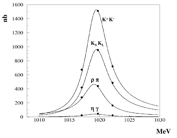
Figure 14: Dependence on $\surd s$ of the cross section for $\phi$-meson production and decay into each of the major modes, $K^{+}$$K^{-}$, $K_{S}$$K_{L}$, $\rho$$\pi$, and $\eta$$\gamma$. Curves show the parameterization used in the MC; points are KLOE measurements from 2002.

5.2 Generators for meson decays

The routines in the geant library simulate two- and three-body decays according to pure phase-space distributions. Only the main decay modes of muons, pions, kaons, and $\eta$ mesons are simulated. We have enriched the list of simulated particle-decay modes to include rare decays and refined the kinematic distributions of the secondaries to include the correlations expected from the matrix elements for the different decay processes.

The generator for $\phi$ events discussed in Sec. 5.1 selects the $\phi$ decay channel and declares the decay products to geant. Initial-state reactions and the beam-energy spread of the machine ($\Delta E_{\mathrm{beam}}/E_{\mathrm{beam}}=0.04\%$ at DAΦNE) are taken into account event by event in the simulation of the decay kinematics.

For $\phi\to K^{+}K^{-}$ and $K_{S}K_{L}$ decays, the kaons are distributed as $\d N/\d\cos\theta\propto\sin^{2}\theta$ in the polar angle.

In the $\phi\to\rho\pi$ channel, the $\rho$ decays dominantly to $\pi\pi$; other possible $\rho$ decays are to $\pi\gamma$, $\eta\gamma$, and $\pi^{\pm}\eta$. The three-body phase space of the secondaries is modified assuming a Breit-Wigner shape for the $\rho$ resonance, with $m_{\rho}=776.1$ MeV/$c^{2}$ and $\Gamma_{\rho}=145.6$ MeV/$c^{2}$ for all three $\rho$ charge states. In $\phi\to\rho\pi$ decays with $\rho\to\pi\pi$, the contribution from direct $\phi\to 3\pi$ decay and the interference between direct and $\rho$-mediated process are simulated, using the values measured by KLOE for the relative contributions from each term [35].

Scalar mesons from radiative $\phi$ decays are distributed as $\d N/\d\cos\theta\propto 1+\cos^{2}\theta$ in the polar angle and are generated by a separate set of routines, which in some cases (e.g., the eva generator, customized for KLOE) offer a choice of production models.

Besides the major modes, the list of neutral-kaon decays simulated includes rare decays such as $K_{S}\to\pi\ell\nu$, $K_{S}\to\pi^{+}\pi^{-}\pi^{0}$, and $K_{S}\to\pi^{0}\pi^{0}\pi^{0}$.

For the simulation of semileptonic kaon decays, kaon decays into two pions, and leptonic decays of charged kaons, radiative corrections are taken into account. In order to avoid problems with divergences at low radiated-photon energy, we use the method of Ref. 36 to sum the amplitudes for virtual and real radiative processes to all orders of $\alpha$. We have verified that the soft-photon approximation used in this treatment is valid for the entire range of photon energies in the kaon decays of interest. Whenever a decay is generated in which the radiated energy is more than 0.1 MeV, a final-state photon is explicitly simulated.

The Dalitz plots for the $K\to 3\pi$ decays are generated according to the form $\left|M\right|^{2}=1+gu+hu^{2}+jv+kv^{2}$, where $u=(s_{3}-s_{0})/m_{\pi^{+}}^{2}$ and $v=(s_{1}-s_{2})/m_{\pi^{+}}^{2}$, while $s_{i}=(P_{K}-P_{i})^{2}$ and $s_{0}=(1/3)\sum s_{i}$. The values of the parameters $g$, $h$, $j$, and $k$ used in the simulation are those published by the PDG [37].

The $\pi^{0}$ decays simulated include the Dalitz decay $\pi^{0}\to e^{+}e^{-}\gamma$. All decay modes of the $\eta$ and $\eta^{\prime}$ mesons are simulated.

5.3 Drift chamber simulation

The chamber geometry as simulated consists of a cylindrical carbon-fiber and aluminum inner wall, a cylindrical carbon-fiber outer wall, and two spherical carbon-fiber endplates. The average material burden contributed by the readout electronics installed on the endplates is also taken into account. The two stiffening rings at the edges of the endplates and the 12 carbon-fiber struts are simulated as well. In order to reduce CPU time consumption, the $52\,000$ wires are not described in the geant geometry as volumes, but their presence is taken into account at the tracking level. All parameters used to describe the chamber geometry are stored in the database.

Tracking in the drift chamber is performed by a dedicated package that uses standard geant routines for particle propagation and for interactions in the medium. The cell geometry is calculated for each tracking step using the wire positions and stereo angles stored in the database; the wire sags are also taken into account. When a particle hits a wire, a multiple-scattering simulation using the appropriate wire material is performed. The energy loss in each cell is also computed.

For each cell crossed, the program computes the distance of closest approach between the track helix and the nearest sense wire. These distances are converted to drift times using $s$–$t$ relations that are parameterized as described in Sec. 4.2. The constants describing the $s$–$t$ relations used for this conversion are obtained from a detailed simulation of the electron drift performed with the garfield program [38].

At the digitization stage, the TDC-signal arrival time is calculated, with the drift time, the particle time of flight, and the propagation time of the signal along the wire taken into account. For cells crossed by more than one particle (or more than once by the same particle), only the signal coming from the first hit is registered. The raw signal arrival times are then written to output banks that serve as the input to the reconstruction program. An algorithm for digitization of the charge values for each wire to simulate the measurements from the recently installed ADCs is currently under development.

The drift-chamber reconstruction of simulated data is essentially identical to that of real data, with two notable exceptions. First, a dedicated reconstruction module allows hits on dead channels to be deleted (the configuration of dead channels during data taking is stored in the database run by run). Second, the $s$–$t$ relations used for the track reconstruction are obtained by the calibration procedure described in Sec. 4.2, using simulated cosmic-ray events.

5.4 Calorimeter simulation

In order to reduce CPU consumption, the geant representation of the calorimeter geometry does not include a detailed description of the individual fibers embedded in the grooved lead plates. An approximate geometry consisting of thin, alternating layers of lead and scintillator is used instead.

The starting point for the simulation of the EmC response is the energy deposition of the incident particle in the active material, $\Delta E$. The light yield collected at each end of a calorimeter module is calculated by correcting $\Delta E$ as a function of the point of impact along the fibers to account for light attenuation. The resulting energy is converted into a number of photoelectrons, $N_{\mathrm{pe}}$, using an average value for the light-yield conversion constant, $Y_{\mathrm{MC}}$, and applying Poisson statistics to simulate the fluctuations.

To each photoelectron, a time is assigned by adding scintillation and light-propagation times to the arrival time of the particle. The number of photoelectrons and the photoelectron times are accumulated for each detector cell, i.e., for the entire volume viewed by each individual PMT. The energy measured for each PMT is obtained by dividing the total number of photoelectrons by $Y_{\mathrm{MC}}$. The final PMT time measurement is obtained from the time distribution of the photoelectrons collected. In order to simulate the behavior of the constant-fraction discriminators used in the experiment, this time is set to the value corresponding to the integration of 15% of the complete signal.

We have made extensive use of $\phi\to\pi^{+}\pi^{-}\pi^{0}$ events in tuning the simulation of the calorimeter. In such events, the energy and momentum of one of the photons can be accurately predicted from the reconstruction of the $\pi^{+}$$\pi^{-}$ vertex and the position alone of the cluster from the other photon. No other calorimetric information is needed.

To establish the thickness of the lead and scintillator planes in the simulated geometry, we have minimized the differences between the shower shapes for photons in data and MC events. Using $\phi\to\pi^{+}\pi^{-}\pi^{0}$ events in the data set, the distribution of the depth of the first plane fired by incident photons of given energy $E_{\gamma}$ and polar angle $\theta_{\gamma}$ has been fit with a discretized exponential function with mean-depth parameter $\lambda$. In Fig. 15a, the dependence of $\lambda$ on $E_{\gamma}$ is shown for different values of $\theta_{\gamma}$. The distributions flatten above 200 MeV, as expected when the cross section for $e^{+}e^{-}$-pair creation approaches the plateau limit corresponding to an interaction length of $7/9\,X_{0}$. The plateau values of the interaction length for different $\theta_{\gamma}$ intervals shown in Fig. 15b correspond to values for $X_{0}$ of $\sim$$1.2$ $\mathrm{cm}$. This is in reasonable agreement with the radiation length estimated a priori from the known composition of the calorimeter modules [2]. Using the same technique, we have also measured the effective radiation length in the Monte Carlo and varied the relative thickness of the lead and scintillator planes in order to establish agreement with data. This procedure leads to a representation of the calorimeter module as 220 layers of 480 $\mu\mathrm{m}$ of lead plus 620 $\mu\mathrm{m}$ of scintillator.

Figure 15: a) Mean interaction-length parameter $\lambda$ as a function of photon energy $E_{\gamma}$ for different intervals in the photon polar angle $\theta_{\gamma}$. b) Limiting (plateau) values of $\lambda$ for different intervals in $\theta_{\gamma}$.

To calibrate the calorimeter response, we have used $\phi\to\pi^{+}\pi^{-}\pi^{0}$ events with particles crossing the center of the calorimeter modules ($s=s_{0}$) to determine the average light-yield conversion constant for data, $Y$, as a function of the energy of the incident particle. The relation between $Y$ and $Y_{\mathrm{MC}}$ is $Y_{\mathrm{MC}}=Yg_{i}(s_{0})/f_{e}$ (recall that $g_{i}$ is the correction factor for light attenuation in the fibers of the $i^{\mathrm{th}}$ cell; $f_{e}$ is the sampling fraction for electromagnetic showers). If Poisson statistics dominate the fluctuations in the energy response, we expect the distributions of the ratios $E^{A}/\!E^{B}$ and $(E^{A}-E^{B})/(E^{A}+E^{B})$, where the values $E^{A,B}$ refer to the energy measurement at each side of the module, to have variances $\sigma=\surd 2/N_{\mathrm{pe}}$. We obtain $Y=0.6$–0.7 $\mathrm{p.e.}$/MeV per side. This has led us to set $Y_{\mathrm{MC}}=19$ $\mathrm{p.e.}$/MeV in the most recent version of the MC. After these adjustments, reasonable agreement between MC and data is observed for the energy response and resolution as a function of $E_{\gamma}$ (see Fig. 16).

Figure 16: Energy response and resolution determined using $\phi\to\pi^{+}\pi^{-}\pi^{0}$ events with photons incident on the calorimeter barrel: a) relative linearity of energy response, $\Delta E_{\gamma}/E_{\gamma}$, as a function of $E_{\gamma}$; b) relative energy resolution, $\sigma(E_{\gamma})/E_{\gamma}$, as a function of $E_{\gamma}$. Solid (open) circles are for data (MC).

With the geometry and response of the calorimeter thus simulated, assuming that the visible energy follows the spectrum of energy loss inside the scintillator, we obtain sampling fractions $f_{e}=11\%$ for electromagnetic showers, and $f_{\mu}=18\%$ for minimum-ionizing particles. The ratio $f_{e}/\!f_{\mu}=0.6$ is 20% lower than the value measured using a test beam. The same discrepancy between MC and data has been found for the position of the minimum-ionizing peak from the most energetic pions in $\phi\to\pi^{+}\pi^{-}\pi^{0}$ events. Samples of $e^{+}e^{-}\to\mu^{+}\mu^{-}(\gamma)$ and $\phi\to\pi^{+}\pi^{-}\pi^{0}$ events in data are currently being used to adjust the average energy loss of pions and muons in the scintillator in order to obtain good MC-data agreement on the calorimeter energy response over the entire momentum range of interest.

The effect of the cracks between the barrel modules is illustrated in Fig. 17, which shows the ratio $(E_{\mathrm{cl}}-E_{\gamma})/E_{\gamma}$ as a function of azimuthal distance from the module boundaries for photons from $\phi\to\pi^{+}\pi^{-}\pi^{0}$ events. A clear deterioration in the response is observed within $\pm 1^{\circ}$ of the module boundaries. This effect is due to fibers broken during the final milling of the modules, and it is not easy to include in the MC given the representation of the geometry in use. We simulate this effect during event reconstruction by weighting the reconstructed energies with a function of the azimuthal positions of the generated hits. A similar effect is observed in the endcaps; in this case, the magnitude of the effect is smaller, and it is not yet corrected for.

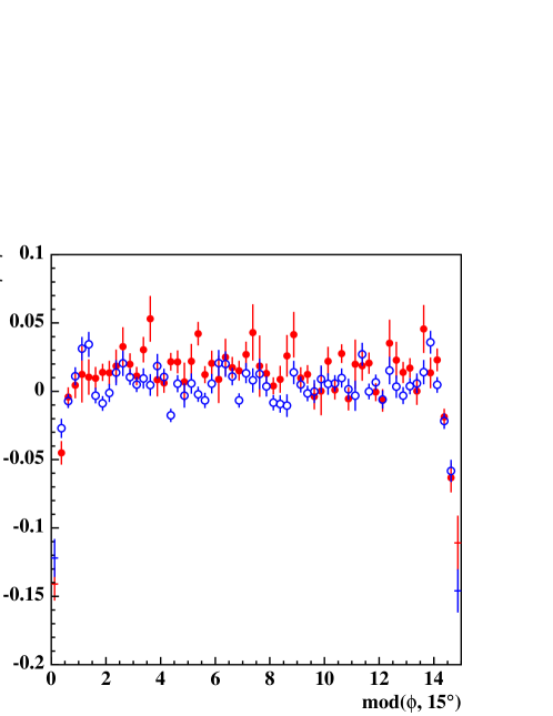
Figure 17: Energy response as a function of the azimuthal distance from the boundaries between modules of the barrel calorimeter. Solid (open) circles are for data (MC).

For the time simulation, the scintillation curve for single photoelectrons has been tuned to reproduce the stochastic contribution to the timing resolution of $54~{}\mathrm{ps}/\surd E(\mbox{GeV})$. The MC-data agreement after the adjustment is reasonable. The constant contribution to the timing resolution observed in data, $\mbox{$\sim$$140$}~{}\mathrm{ps}$, is mostly due to jitter introduced when rephasing the trigger with the machine RF signal. To simulate this effect, an offset sampled from a Gaussian with a width of 140 $\mathrm{ps}$ is added in common to all time signals in the event.

5.5 Trigger simulation

The KLOE trigger is emulated in software during event reconstruction. Non-triggering events are retained in the output, but the result of the trigger emulation is encoded in the data stream, allowing MC estimates of the trigger efficiency to be obtained.

For the emulation of the EmC trigger, the energy deposited in each calorimeter element and the PMT-signal arrival times are first read out. For each trigger sector, the energies of all cells fired within a coincidence window of 3.5 $\mathrm{ns}$ are summed, where this interval approximately corresponds to the width of the actual PMT signals. By comparison to a set of discriminators reproducing the hardware circuitry, these sums are transformed into logic signals of 70-$\mathrm{ns}$ duration. Three different sets of thresholds are used to distinguish $\phi$ decays, Bhabha events, and cosmic-ray events. The threshold values are determined from the analysis of real data on a run-by-run basis. The resulting logic signals are used to compute the multiplicity of hit sectors on the barrel and each of the two endcaps, and finally combined to produce the $\phi$, Bhabha, and cosmic-ray trigger signals.

The signals from the DC wires are read out and shaped at 250 $\mathrm{ns}$. As in the hardware, the signals from wires in different groups of adjacent DC planes are summed. These “superlayer” signals are then summed in turn to get the effective DC multiplicity as a function of time. A level-1 DC trigger is set whenever this sum exceeds a given threshold. The sum is then integrated over a 1.2 $\mu\mathrm{s}$ interval and compared to another threshold to define the level-2 DC signal. The values of these two thresholds are determined from the analysis of real data on a run-by-run basis.

Finally, the DC- and EmC-trigger signals are combined to deliver the final level-1 and level-2 trigger decisions with the correct timing relative to the start of the event as generated. Once the trigger time has been simulated, it is rounded to the next highest multiple of $4t_{\mathrm{RF}}$ to simulate the rephasing of the experiment’s level-1 trigger with the machine clock. A time interval corresponding to an integer number of bunch crossings from one to four is then subtracted from the rephased trigger time; this corresponds to randomly specifying the particular bunch crossing that produced the event. The result is the simulated value of $t_{0,\,\mathrm{evt}}$; this value is then applied to the times of all calorimeter and drift-chamber hits.

5.6 Machine background simulation

A detailed simulation of detector activity from the accidental coincidence of hits from machine background is required in order to obtain the high precision and careful control of systematics needed for most KLOE physics analyses. This activity consists mainly of noise hits in the DC and low-energy clusters in the EmC, mostly at small angles. Background hits in the chamber and calorimeter are added to the simulated events at the reconstruction stage.

For the 2001–2002 data, this background was obtained from $e^{+}e^{-}\to\gamma\gamma$ events satisfying specific topological cuts. These events are selected from KLOE data with a cross section of $\sim$$40$ $\mathrm{nb}$. Since $e^{+}e^{-}\to\gamma\gamma$ events are fully neutral, all DC hits in these events are considered background, in addition to all EmC clusters not identified as belonging to the $\gamma\gamma$ topology (care is taken to correctly distinguish clusters from initial state radiation or from cluster splitting, which actually belong to the $\gamma\gamma$ topology, from those due to machine background).

A file containing background hits is created for each raw file in the data set. As discussed in Sec. 5.7, an MC run corresponds to a set of raw files in data. We insert the hits from each event in the set of background files into multiple events in the corresponding MC run, with a reuse factor chosen to ensure that all background events are used roughly the same number of times. This ensures reproduction of the time-variable background spectrum in the simulated output.

For both the EmC and DC, when hits are inserted, their timing relative to the start time of the $\gamma\gamma$ event from which they were extracted is preserved. The insertion takes place before the trigger simulation is performed, so that simulated and inserted hits are temporally aligned. Hit-blocking effects are reproduced. In the drift chamber, a background hit that arrives earlier than a simulated hit on the same wire causes the simulated hit to be removed from the event, and vice versa. On the calorimeter, if both a background hit and a simulated hit occupy the same cell, the earlier arrival time on each side of the cell is retained, while the energy read out at each side is taken from the sum of the two hits. The trigger simulation is then performed, and the simulated and inserted hits are then $t_{0}$-smeared simultaneously using the algorithm of Sec. 5.5.

For the drift chamber, the $s$–$t$ relations used for simulated events and for real data are sufficiently similar so that all hits—simulated and inserted—can be reconstructed with the MC $s$–$t$ relations. A correction is made to the energy scale when calorimeter hits are inserted. This correction ensures that the inserted calorimeter hits reconstruct with the same energy that they had in the data event from which they were extracted.

5.7 Monte Carlo production campaigns

An extensive simulation campaign for the 2001–2002 KLOE data set is currently near completion. This campaign is focused on the production of general-purpose samples, such as samples in which all decays of the $\phi$ are present in proportion to their natural branching ratios, or in which the $\phi$ always decays to $K_{S}$$K_{L}$ but all possible final states are present. Such samples are particularly useful for understanding backgrounds in studies of rare decays. The production procedure is geared towards providing high-statistics samples. The total number of events in each sample is established using an effective luminosity scale factor, which ranges from 0.2 for general-purpose simulations such as $\phi\to\mbox{all}$ (peak cross section $\sim$$3.1$ $\mu\mathrm{b}$), to 5 for dedicated simulations such as $e^{+}e^{-}\to\pi^{+}\pi^{-}\gamma$ (cross section $\sim$$50$ $\mathrm{nb}$). In all, current plans call for the production of about $10^{9}$ events.

In order to track run-by-run variations in the operating conditions of the collider and detector, an MC sample is generated for each run in the data set, with the number of events proportional to the integrated luminosity of the run under simulation, and such parameters as machine energy, momentum of the collision center-of-mass, beam-spot position, map of dead detector elements, and trigger thresholds set to correspond to the run conditions. Background hits in the EmC and DC are inserted with special care in order to ensure reproduction of the background spectra resulting from variations with time within each run (see Sec. 5.6). As a result of these procedures, time-variable conditions are correctly averaged in the sample of MC events corresponding to any given group of runs in the data set.

For the production of a given sample, one job is submitted for each run in the data set. A production job handles generation, reconstruction, and DST creation. In order to have intermediate files of reasonable size, it is usually necessary to split the generation into several processes. A reconstruction process immediately follows each generation process. DSTs are made after all generation and reconstruction is complete. Production is started by submitting a large number of jobs to a batch queue managed by IBM’s LoadLeveler utility [16].

When MC events are reconstructed, several algorithms intended to complete the simulation are run before any of the actual reconstruction algorithms. Background hits in the EmC and DC are first inserted. Hits on dead wires of the drift chamber are next removed. The trigger emulator is then run, after which hits on hot drift-chamber wires can be removed (in the reconstruction of real data, they are removed at the input stage). Finally, the $t_{0}$-smearing algorithm is applied. After these steps, the same algorithms used for the reconstruction of real data are run, in the same order described in Sec. 3.1.

The only other special treatment given to MC events concerns the behavior of the machine-background filter and the event-classification module. Like the trigger emulator, these modules only record their decisions in the output file; they do not actually suppress events. In particular, MC events are not divided up into streams at the reconstruction stage; only one reconstruction output file is produced from each generator output file.

The reconstruction output file contains enough information to allow recovery of the events as generated, before the introduction of background hits. Therefore, only the reconstructed output files are archived; generator output files are discarded.

In the last stage of the production job, DSTs are produced. The same five types of DSTs as for real data can be produced for MC events, with the application of the same stream-specific algorithms described in Sec. 3.2. However, for the production of dedicated MC samples (e.g., for the process $e^{+}e^{-}\rightarrow\pi^{+}\pi^{-}\gamma$), only the DST types of interest are produced. Event streaming is performed at the DST-production stage. In addition to all events classified on the basis of reconstructed quantities, each MC DST stream contains all events with topologies as-generated relevant to the physics of the stream. MC DSTs also contain a minimal set of information about the true event topology. All information in the geant KINE and VERT banks is present in the DSTs, but there is no information about individual hits. In place of the hit banks themselves, the correspondences between reconstructed topologies (clusters, tracks) and simulated particles (KINE tracks) are kept. Like data DSTs, MC DSTs are archived and recalled to the NFS-mounted disk cache for prompt access.

Table 4 gives a statistical summary of the Monte Carlo production campaigns completed to date. In the two general-purpose production campaigns, $\phi\rightarrow\mathrm{all}$ and $\phi\rightarrow K_{S}K_{L}$, the entire 2001–2002 data set ($\sim 450~{}\mathrm{pb}^{-1}$) was simulated at luminosity scale factors of 0.2 and 1, respectively. Events such as these require 200 $\mathrm{ms}$ to generate and 175 $\mathrm{ms}$ to reconstruct on the CPUs in the B80 servers; the running times in the table were obtained with 60 CPUs. For the $e^{+}e^{-}\rightarrow\pi\pi\gamma$ campaign, only the 2001 data were simulated ($\sim 170~{}\mathrm{pb}^{-1}$), at a luminosity scale of 5. In these three campaigns, a total of $7\times 10^{8}$ events were produced in about three months of real time.

Program	Events ($10^{6}$)	CPU time (days)	Output size (TB)
$\phi\rightarrow\mathrm{all}$	255	1100	6.9
$\phi\rightarrow K_{S}K_{L}$	410	1800	11.0
$e^{+}e^{-}\rightarrow\pi\pi\gamma$	36	110	0.8

Table 4: Statistics for some Monte Carlo production campaigns completed to date

6 Conclusions

The high event rate at DAΦNE—1.5 $\mathrm{kHz}$ of $\phi$ decays accompanied by a similar yield of Bhabha events within the acceptance, which must be downscaled, and of machine-background and cosmic-ray events, which must be rejected—has required us to design and operate a large, complex, and reliable system for data acquisition and offline data processing.

The DAQ system described in Ref. 5 has guaranteed a bandwidth of 3 $\mathrm{kHz}$ during data taking, while simultaneously handling various tasks related to data-quality control and subdetector calibration and monitoring. At present, the mass-storage and data-handling systems manage over 100 $\mathrm{TB}$ of raw data and a comparable amount of reconstructed data both from the detector and from the experiment’s Monte Carlo.

We have carefully designed and optimized the offline software environment to ensure that data is reconstructed immediately following acquisition. As part of this effort, we have developed various tools for detector calibration, access to reconstructed data, process scheduling, and the like. We have placed special emphasis on maximizing the efficiency and precision of the reconstruction program. As a result, the performance specifications of the detector—momentum and vertex resolution for the drift chamber and energy and time resolution for the calorimeter—have been fully satisfied.

At the same time, we have implemented a continuing series of improvements to the simulation of the detector response, the representation of machine background, and the accuracy of the physics generators in the experiment’s Monte Carlo. As a result of this development program, excellent agreement between data and Monte Carlo has been obtained for the distributions of key variables, and the Monte Carlo has become a reliable and important tool for physics analysis.

We have dedicated a significant amount of work to the construction of a stable, scalable data-processing system with the flexibility to exploit all of the available resources. During the past four years of operation, we have implemented a series of important upgrades to keep pace with the growing demands of the experiment. With the upgrades already scheduled for 2004, the environment will be well suited to handle predicted increases in the DAΦNE luminosity.

References

- [1] M. Adinolfi, et al., The tracking detector of the KLOE experiment, Nucl. Instrum. Meth. A 488 (2002) 51.
- [2] M. Adinolfi, et al., The KLOE electromagnetic calorimeter, Nucl. Instrum. Meth. A 482 (2002) 364.
- [3] M. Adinolfi, et al., The QCAL tile calorimeter of KLOE, Nucl. Instrum. Meth. A 483 (2002) 649.
- [4] M. Adinolfi, et al., The trigger system of the KLOE experiment, Nucl. Instrum. Meth. A 492 (2002) 134.
- [5] A. Aloisio, et al., Data acquisition and monitoring for the KLOE detector, Nucl. Instrum. Meth. A 516 (2004) 288.
-
[6]
G. Cabibbo, et al., The calibration of the space-time relations in the KLOE
drift chamber, KLOE Note 175 (2002).
URL http://www.lnf.infn.it/kloe/pub/knote/kn175.ps -
[7]
L. Williams, et al., HEPDB, reference manual, version 1.19, CERN Program
Library Long Writeup Q180 (1995).
URL http://wwwasdoc.web.cern.ch/wwwasdoc/hepdb_html3/hdbmai%n.html -
[8]
IBM Tivoli Storage Manager.
URL http://www.ibm.com/software/tivoli/products/storage-mgr -
[9]
KLOE Collaboration, I. Sfiligoi, et al., KID - KLOE Integrated
Dataflow, in: Proceedings of CHEP 2001 (Beijing, 3–7 Sep. 2001),
Science Press, Beijing, 2001.
URL http://www.lnf.infn.it/kloe/pub/doc/ka082.pdf -
[10]
DB2 Product Family.
URL http://www.ibm.com/software/data/db2 -
[11]
I. Sfiligoi, KLOE database - the bookkeeping and computing system catalogue,
KLOE Note 184 (2003).
URL http://www.lnf.infn.it/kloe/pub/knote/kn184.pdf -
[12]
E. Sexton-Kennedy, M. Shapiro, D. R. Quarrie, A beginner’s guide to
Analysis_Control and Build_Job, CDF Note 384 (1996).
URL http://www-cdf.fnal.gov/offline/a_c/a_c.html -
[13]
Concurrent Versions System.
URL http://www.cvshome.org -
[14]
D. R. Quarrie, B. Troemel, YBOS programmer’s reference manual (1992).
URL http://www-cdf.fnal.gov/offline/ybos/murat/ybos.01.html -
[15]
J. Gailly, M. Adler, zlib 1.1.4 manual (2002).
URL http://www.gzip.org/zlib/manual.html -
[16]
LoadLeveler V2.2.
URL http://www.ibm.com/servers/eserver/ecatalog/us/software - [17] A. Antonelli, et al., Short description of the track reconstruction program with the KLOE drift chamber, KLOE Memo 194 (1998).
- [18] H. Albrecht, et al., Nucl. Instrum. Meth. A 275 (1989) 1.
- [19] P. De Simone, et al., Cell response parameterization, KLOE Note 98 (1994).
-
[20]
M. Primavera, S. Spagnolo, Parametrization of the time to distance
relations and resolution in the KLOE drift chamber, KLOE Note 165 (1997).
URL http://www.lnf.infn.it/kloe/pub/knote/kn165.ps - [21] A. Antonelli, et al., Momentum calibration of the KLOE drift chamber, KLOE Memo 231 (2001).
- [22] A. Antonelli, et al., The KLOE field map revisited, KLOE Memo 233 (2001).
- [23] KLOE Collaboration, A. Aloisio, et al., Phys. Lett. B 538 (2002) 21.
-
[24]
M. Palutan, T. Spadaro, P. Valente, Measurement of
with
KLOE 2000 data, KLOE Note 174 (2002).
URL http://www.lnf.infn.it/kloe/pub/knote/kn174.ps.gz - [25] C. M. Carloni Calame, et al., Nucl. Phys. B 584 (2000) 459.
- [26] C. M. Carloni Calame, et al., The BABAYAGA event generator, hep-ph/0312014 (2003).
- [27] C. D. Buchanan, et al., Phys. Rev. D 45 (1992) 4088.
- [28] R. Brun, et al., GEANT3, CERN-DD/EE/84-1 (1984).
- [29] R. Brun, et al., GEANT: Simulation program for particle physics experiments, user guide and reference manual, CERN-DD-78-2-REV (1978).
- [30] F. A. Berends, R. Kleiss, Nucl. Phys. B 228 (1983) 537.
- [31] H. Czyż, et al., The radiative return at - and -factories: FSR at next-to-leading order, hep-ph/0308312 (2003).
- [32] F. Binner, J. H. Kühn, K. Melnikov, Phys. Lett. B 459 (1999) 279.
- [33] N. N. Achasov, V. V. Gubin, Phys. Rev. D 63 (2001) 094007.
- [34] F. A. Berends, R. Kleiss, Nucl. Phys. B 260 (1985) 32.
- [35] KLOE Collaboration, A. Aloisio, et al., Phys. Lett. B 561 (2003) 55.
- [36] S. Weinberg, Phys. Rev. 140 (1965) 516.
- [37] Particle Data Group, K. Hagiwara, et al., Phys. Rev. D 66 (2002) 010001.
- [38] R. Veenhof, et al., GARFIELD, a drift-chamber simulation program, User’s guide, version 5.05, CERN Program Library (1994).