The Capabilities of the EISCAT Svalbard Radar for Inter-hemispheric Coordinated Studies

Abstract

In this article we want to present the EISCAT Svalbard Radar (ESR) in some detail, as well as some of the instruments of interest for ionospheric and magnetospheric research that are located in the vicinity of it. We particularly describe how this instrument cluster, close to the geomagnetic conjugate point of the Chinese Antarctic Zhongshan station, can contribute to inter-hemispheric coordinated studies of the polar Ionosphere.

Keywords: EISCAT, Incoherent Scatter Radar, Conjugate studies

1 The Incoherent Scatter Technique

The use of incoherent scatter radars as a powerful ground-based diagnostic tool for studying the near-Earth space environment began with the first theoretical predictions by Gordon (1958), and the first observations by Bowles (1958) a few months later. There are several comprehensive reviews of the Incoherent Scatter technique, (e.g. Evans, 1969, 1975; Bauer, 1975; Beynon and Williams, 1978), while an overview of the early history of Incoherent Scatter, as well as an updated description of the theory, instruments and signal processing involved can be found in (Farley, 1996).

The term Incoherent Scatter (IS) from an ionized gas refers to the extremely weak scatter from fluctuations in plasma density caused by the random thermal motion of the ions and electrons. Due to the very low radar scattering cross section of an individual electron, only about $1.0\times 10^{-28}\,\mathrm{m^{2}}$, the total cross section of all the electrons in ten cubic kilometers — a typical volume probed in an experiment — of the ionosphere with a maximum density of the order of $10^{12}\,\mathrm{m^{-3}}$ is only about $10^{-6}\,\mathrm{m^{2}}$. To detect signal from this weak source, we need a radar capable of detecting a coin at $300\,\mathrm{km}$ distance!

Incoherent Scatter Radars (ISR) therefore consist of large antennas, powerful transmitters, and sensitive and sophisticated receiver systems, since in addition to measuring the signal and its power we also need to measure the full Doppler power spectrum or equivalently the auto correlation function (ACF) of the back-scattered signal.

When the radar frequency, ${\omega}_{\mathrm{radar}}$ is much higher than the plasma frequency ${\omega}_{p}$, the radar wave travels almost unperturbed through the very dilute ionospheric plasma. A small fraction of the wave energy is deposited into the acceleration of the electrons, which radiates back as small dipoles. The ions also absorb energy in this process, but due to their relatively high mass, their radar scattering cross section is a factor $(m_{e}/m_{i})^{2}$ smaller than the electron radar scattering cross section, and their contribution to the scattered signal is negligible.

In the pioneering work by Gordon, he assumed that one would see “true” incoherent scattering from the individual free electrons. This would result in a back-scattered power spectrum with a width proportional to the electron thermal velocity. The first experiments, however, showed a power spectrum with a width proportional to the ion thermal velocity, with the power contained in a much narrower frequency range than predicted. This dramatically improved the signal to noise ratio within this frequency range. Despite the fact that the electrons are the scattering particles in this process, they are, due to their low mass, highly mobile and will therefore easily follow the heavier ions through electromagnetic interactions. The typical scale size of these interactions is called the Debye length. For a typical incoherent scatter radar configuration, the radar wavelength is much larger than the Debye length of the ionospheric plasma, and the power spectrum of the received signal carries information about the plasma as a whole, with the electron dynamics strongly influenced by the ions. For the situation with the radar wavelength shorter than the Debye length, we have “true” incoherent scattering, and the electrons scatter as free particles, with a received power spectrum typical for the electron velocity distribution function.

The scattered signal contains information about the plasma density, the electron and ion temperatures, the ion composition, the bulk plasma motion, and various other parameters and properties of the probed plasma.

A number of different approaches all lead to the same result for the incoherent scatter power spectral shape (Fejer, 1960; Dougherty and Farley, 1960; Salpeter, 1960; Rosenbluth and Rostoker, 1962; Rostoker, 1964; Trulsen and Bjørnå, 1975), and this back-scattered power spectrum can be given by the equation:

$$\begin{split}S(\boldsymbol{k},{\omega})={}&N_{e}\left|1-\frac{{\chi}_{e}(\boldsymbol{k},{\omega})}{{\epsilon}(\boldsymbol{k},{\omega})}\right|^{2}\int d\boldsymbol{v}f_{e}(\boldsymbol{v}){\delta}({\omega}-\boldsymbol{k}\cdot\boldsymbol{v})\\ &{}+\sum_{i}N_{i}\left|\frac{{\chi}_{e}(\boldsymbol{k},{\omega})}{{\epsilon}(\boldsymbol{k},{\omega})}\right|^{2}\int d\boldsymbol{v}f_{i}{\delta}({\omega}-\boldsymbol{k}\cdot\boldsymbol{v})\end{split}$$ (1)

where the electric susceptibility ${\chi}_{{\alpha}}(\boldsymbol{k},{\omega})$ for species $\alpha$ is given by

$${\chi}_{{\alpha}}(\boldsymbol{k},{\omega})=\frac{{\omega}_{pe}^{2}}{k^{2}}\int_{L}\frac{\boldsymbol{k}\cdot{\delta}_{\boldsymbol{v}}f_{{\alpha}}(\boldsymbol{v})}{{\omega}-\boldsymbol{k}\cdot\boldsymbol{v}}\,d\boldsymbol{v},$$ (2)

the dielectric constant function ${\epsilon}(\boldsymbol{k},{\omega})$ is given by

$${\epsilon}(\boldsymbol{k},{\omega})=1+{\Sigma}_{{\alpha}}{\chi}_{{\alpha}}(\boldsymbol{k},{\omega}),$$ (3)

and $f_{{\alpha}}(\boldsymbol{v})$ the velocity distribution function for the species ${\alpha}$.

Equation (1) gives rise to two parts of the power spectrum, the ion line (from the second term) and the plasma line (from the first term) respectively. The portions of the power spectrum with small Doppler shifts is often referred to as the ion line. It can be viewed as two very broadened overlapping lines corresponding to damped ion-acoustic waves traveling parallel and anti-parallel to the $\boldsymbol{k}$-vector determined by the radar system; toward and away from the radar for a mono-static system. The lines have Doppler shifts corresponding to the frequency of ion-acoustic waves, which are solutions of equation (1) in the low frequency range. From the ion-line we are able to determine a range of plasma parameters:

The electron density, $N_{e}$ can be found from the total back-scattered power. The constant of proportionality between the electron density and the back-scattered power depends on the electron and ion temperature ($T_{e}$ and $T_{i}$).
The temperature ratio, $T_{e}/T_{i}$ can be determined from the ratio of the peaks to the dip in the ion spectra (shown in figure 1, panel 1) due to the $T_{e}/T_{i}$ dependence in the ion-acoustic damping term.
The ion temperature to mass ratio, $T_{i}/m_{i}$ can be found from the width of the ion spectra. If $m_{i}$ is known (e.g. from a model), $T_{i}$ can be found, and hence $T_{e}$.
Line-of-sight ion velocity can be determined from the Doppler shift of the ion spectra (shown in figure 1, panel 2). By using a tristatic radar, the drift can be determined in three directions, and hence the full ion velocity vector can be found.

The analysis is done by fitting all parameters simultaneously in an iterative process. Behind this fitting routine, the most severe assumptions are the homogeneity and stationarity assumed over the whole scattering volume and the whole integration time. For quiet conditions these assumptions are sufficiently fulfilled, but during active and disturbed periods, the returned power is sometimes increased by one or two order of magnitude, the plasma is driven out of thermal equilibrium, and the ion-line can be strongly asymmetric with one or both of the ion-acoustic shoulder enhanced (Sedgemore-Schulthess and St.-Maurice, 2001, and references therein). During these periods, the fitting process does not work, since it assumes the plasma to be in thermal equilibrium, and we are not able to determine the plasma parameters from the spectra. The processes behind these “anomalous” ion spectra are not yet fully understood, and more work has to be done in order to understand them, before we will be able to to analyse data also from these periods.

For much higher frequencies, two narrow less damped lines, the plasma lines are found, one up- and one down-shifted. They are high frequency solutions of equation (1). Their frequency depends directly on the electron density, with a small correction from electron temperature, and they can therefore be used to determine these plasma parameters when measured.

Figure 1: Figure a) shows the $T_{e}/T_{i}$ dependence on the ion spectra, and figure b) shows the effect of plasma drift.

2 EISCAT and the ESR

EISCAT was founded by the six European countries France, Great Britain, Germany, Norway, Finland and Sweden in 1975 for the purpose of constructing an ISR at high latitude; right underneath the auroral zone. The EISCAT UHF radar — situated outside Tromsø, Norway — was inaugurated in 1981. It is a tristatic system, the only one in operation in the world today, meaning that in addition to the transmitter and receiver in Tromsø, there are passive receivers on two other sites: Sodankylä in Finland and Kiruna in Sweden. The three sites give the radar its unique capability of obtaining true vector velocities in a single common volume. The EISCAT VHF radar, co-located with the UHF radar, became operational in 1985, and extended the capabilities of the EISCAT system in the extreme low- and high-altitude regimes. The mainland EISCAT radars were described in (Folkestad et al., 1983), but the UHF transmitters and all receiver systems have since been totally redesigned, so this description is now out of date. A summary of the EISCAT mainland radars’ capabilities as of the summer of 2001 is given in table 1.

The EISCAT Svalbard Radar (ESR) was inaugurated in August 1996, the same year that Japan became the seventh member of EISCAT. It is situated on top of Mine 7 on the Breinosa mountain $12\,\mathrm{km}$ outside Longyearbyen, the biggest settlement in the Svalbard archipelago. The ESR System is described in detail in (Wannberg et al., 1997). Since then, the transmitter has been upgraded to $1\,\mathrm{MW}$ peak power, and a second antenna, $42\,\mathrm{m}$ in diameter and fixed to point along the geomagnetic field, has been added. A summary of the ESR parameters is given in table 2.

Location	Tromsø		Kiruna	Sodankylä
Geograph. Coordinates	69°35´N		67°52´N	67°22´N
	19°14´E		20°26´E	26°38´E
Geomagn. Inclination	77°30´N		76°48´N	76°43´N
Invariant Latitude	66°12´N		64°27´N	63°34´N
Band	VHF	UHF	UHF	UHF
Frequency (MHz)	224	929	929	929
Max. TX bandwith (MHz)	3	4	-	-
Transmitter	2 klystrons	2 klystrons	-	-
TX Channels	8	8	-	-
Peak power (MW)	$2\times 1.5$	2.0	-	-
Average power (MW)	$2\times 0.19$	0.3	-	-
Pulse duration (msec)	.001–2.0	.001–2.0	-	-
Phase coding	binary	binary	binary	binary
Min. interpulse (msec)	1.0	1.0	-	-
System temp. (K)	250-350	70-80	30-35	30-35
Receiver	analog-digital	analog-digital
Digital processing	14 bit ADC,
	Lag profiles 32 bit complex
Antenna	cylinder	dish	dish	dish
	$120\,\mathrm{m}\times 40\,\mathrm{m}$	$32\,\mathrm{m}$	$32\,\mathrm{m}$	$32\,\mathrm{m}$
Feed system	line feed,	Cassegrain	Cassegrain	Cassegrain
	128 crossed dipoles
Gain (dBi)	46	48	48	48
Polarization	circular	circular	any	any

Table 1: Table summarising the EISCAT mainland radars

Location		Longyearbyen
Geograph. Coordinates		78°09´N
		16°02´E
Geomagn. Inclination		82°06´N
Invariant Latitude		75°18´N
Band		UHF
Frequency (MHz)		500
Max. TX bandwith (MHz)		10
Transmitter		16 klystrons
TX Channels		Continuously tuneable
Peak power (MW)		1.0
Average power (MW)		0.25
Pulse duration (msec)		$<.001-2.0$
Phase coding		binary
Min. interpulse (msec)		0.1
Receiver		analog-digital
System temp. (K)		55-65
Digital processing		12 bit ADC,
		lag profiles 32 bit complex
	Antenna 1		Antenna 2
Antenna	dish		dish
	$32\,\mathrm{m}$		$42\,\mathrm{m}$ Fixed
Feed system	Cassegrain		Cassegrain
Gain (dBi)	42.5		45
Polarization	circular		circular

Table 2: Table summarising the EISCAT Svalbard radars

The EISCAT mainland radars situated in the Auroral zone and the ESR in the vicinity of the Cusp and Polar Cap boundary, constitute an ideal system for the exploration of the Arctic Ionosphere. The ESR is the world’s most modern IS radar, with capabilities matching or exceeding all others. Although some other radars can boast larger antennas or more powerful transmitters, and hence higher sensitivity, the ESR with its TV-type transmitter is capable of higher duty cycle than any other IS radar, which helps to make up for a smaller instrument. The modern receiver system has a flexibility and programmability which gives users a large number of options when it comes to creating their own experiments. This is particularly true of the new hardware upgrade of the mainland radars, which will soon be installed on Svalbard as well. The experiment catalogue for the radars contain experiments which cover the entire Ionosphere from $70$ to $>1200\,\mathrm{km}$, with new experiments under development.

Despite most radar scientists’ discussion of the (power) spectra of the incoherent scattering, the quantity actually measured (or estimated) by the radar is its Fourier transform equivalent, the autocorrelation function (ACF) of the scattering through lagged products of samples of the scattered signal. The EISCAT radars, instead of forming ACF estimates from each of a given number of ranges (called gates), sum and store all such lagged products in a lag profile matrix. Any sufficiently advanced analysis can then use the information from all lagged products that contribute to the scattering from a given range to infer the macroscopic plasma parameters at this range. When such analysis is done on an entire ionospheric profile at once, this is called full profile analysis (Holt et al., 1992). Although full profile analysis has been demonstrated (Holt et al., 1992; Lehtinen et al., 1996), it is not yet in common use for IS radar data.

The spectra that are presented in the following section are formed from the lag profile matrix by summing lagged products in such a way that the regions contributing to the measurement are roughly equivalent for the different lags of the autocorrelation function, thus producing a spectrum from a fairly well-defined and limited region of space.

2.1 Examples of observations

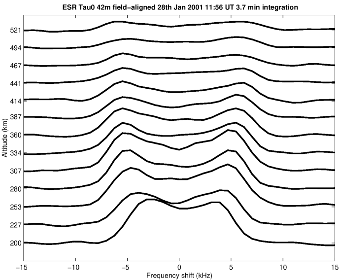
Figure 2: Example of spectra taken using the tau0 experiment on the $42\,\mathrm{m}$ (field-aligned) antenna of the ESR. These spectra have been obtained using $3.7\,\mathrm{min}$ integration.

The mainland EISCAT radars were situated in a valley in order to eliminate the problem of unwanted scattering from the ground, so-called ground clutter. The close-in mountains scatter only at such short ranges that the receiver has not yet been opened, while shielding any solid scatterers at longer ranges. With its location on a mountain, the ESR has no such shielding and, for its first few years of operation, the problem of eliminating ground clutter restricted the lower range of its observations to approximately $150\,\mathrm{km}$ beyond the range of the farthest mountain visible from the site. During this period, an experiment consisting of four long pulses (uncoded) called gup0 was used almost exclusively.

With the solution of the ground clutter problem (Turunen et al., 2000), a new experiment called gup3 was introduced as the standard experiment in 1999. This experiment combines long pulses and alternating codes (Lehtinen and Häggström, 1987), with the alternating codes covering the $E$ and lower $F$ regions, and the long pulses extending coverage into the topside Ionosphere.

More recently, an experiment called tau0, using alternating codes exclusively, has been adopted as the standard experiment at the ESR. This experiment provides coverage from $90$ to $1100\,\mathrm{km}$, and is typically used with $6.4\,\mathrm{s}$ time resolution, although $12.8$ and $3.2\,\mathrm{s}$ have been used on occasion. In figure 2, we show a typical example of tau0 spectra at $F$-region altitudes, using $3.7\,\mathrm{min}$ integration. We observe how the width of the spectra increase with altitude, indicating higher ion temperatures, and how the scattering power decreases, indicating lower electron densities.

2.2 Analysed data

As discussed above, we can infer a number of macroscopic plasma parameters from the power spectrum or ACF of the scattering. This process is called the analysis of the (raw) data, and the result is called analysed data. The program used for analysis of EISCAT data is called GUISDAP, or Grand Unified Incoherent Scatter Design and Analysis Program (Lehtinen and Huuskonen, 1996).

In colour plate 1, we have plotted $96\,\mathrm{hours}$ of an 18-day continuous experiment conducted on February 5.–23., 2001. This experiment illustrates the reliability of the radar and its capability of obtaining long time series observations. In the plate, we can see how the electron density and temperature decreases during nighttime, and the extreme variability of the polar ionosphere. Such data are available from the online analysed data archive at www.eiscat.uit.no, through the MADRIGAL database.

3 Other instrumentation on Svalbard

The excellent facilities of the ESR are further strengthened by a number of instruments located in the immediate vicinity of the ESR or with overlapping fields of view. Also mentioned here are instruments in the vicinity of the magnetic conjugate point of the ESR.

The University of Tromsø owns an optical aurora station operated by the University courses on Svalbard (UNIS) in Adventdalen, outside Longyearbyen, and many universities and institutions around the world have their instruments at the station. In particular the Optics Group at the Geophysical Institute, University of Alaska contribute both with instruments and finances. Amongst the instruments hosted at the station are various all-sky cameras, a Meridian Scanning Photometer (MSP), an Auroral Spectrograph, a Michelson Interferometer, several Eber-Fastie Spectrometers, and magnetometers. Sigernes et al. (2002). Correspondingly, the Zhongshan station is equipped with all-sky TV cameras (e.g. Hu Hongqiao et al., 1999),

In 1995, an $8\times 8$ beam Imaging Riometer for Ionospheric Studies (IRIS) was installed in Adventdalen, close to the auroral station, with contributions from the Danish Meteorological Institute (DMI), the National Institute of Polar Research of Japan (NIPR), UNIS of Longyearbyen and the University of Tromsø. Equivalent instruments are also installed at the South Pole station, at the Antarctic Syowa and Zongshan stations, at Equaliut in Canada, Søndre Strømfjord and Danmarkshavn on Greenland, Tjørnes on Iceland, Kilpisjärvi in Finland and outside Ny-Ålesund on Svalbard (Stauning, 1998). The riometer measures the absorption of cosmic radiation, an absorption usually caused by energetic precipitation penetrating to the lower Ionosphere. The instrument has 64 antennas which are used to form 64 beams covering an area of $240\times 240\,\mathrm{km}$ at $90\,\mathrm{km}$ altitude, and the instrument obtains a full image every second. A closer description of the instrument and its operations is given in (Detrick and Rosenberg, 1990).

The SOUSY HF radar is situated at the foot of the mountain of the ESR. It is a phased-array system using 356 Yagi antennas with a 4° wide beam at the zenith, or 5° zenith angle in either of the NE, NW, SE or SW directions, and an operating frequency of $53.5\,\mathrm{MHz}$ (Röttger, 2000). Being an MST radar, it is suited for observations of the stratosphere, mesosphere and thermosphere, and in particular Polar Mesospheric Summer Echoes (PMSE)

Svalbard is also covered by the CUTLASS pair of the Arctic Dual Auroral Radar Network (SuperDARN). The Arctic SuperDARN network covers most of the Auroral zone (except Siberia), and provides good wide-area convection pattern coverage around Svalbard (Greenwald et al., 1995). In the Antarctic, another network of SuperDARN radars is under development, with the Eastward field of view of the Syowa station covering the area around the Zhongshan and Davis stations (Ogawa, 1996).

The University of Leicester, UK, operated an ionosonde in Longyearbyen until recently. The instrument is not operational at the moment, but it will be moved to the SPEAR (described below) site for reactivation shortly.

In addition, a heating facility called Space Plasma Exploration by Active Radar (SPEAR) is under construction beside the ESR (Wright et al., 2000). Like the heating facility outside Tromsø, this facility can be used for ionospheric modification experiments, induced plasma lines, and to produce $E$-region irregularities which will act as scatterers for the SuperDARN HF radars.

Ny Ålesund, $\approx 150\,\mathrm{km}$ Northwest (magnetically almost North) of Longyearbyen is a busy research community, and in addition to the instruments already mentioned, it hosts a rocket launching facility (SvalRak) which is used for the launch of ionospheric research rockets; since the launch site is at 79° North it is ideally located for scientific exploration of the dayside aurora and processes in the magnetospheric boundary layer (Maynard et al., 2000). The Alfred Wegener Institute for Polar and Marine Research operates a multiwavelength Lidar facility at Ny Ålesund, which monitors mainly the middle atmosphere, but which can link temperature measurements from the ionosphere with those from the neutral atmosphere at the mesopause (Neuber et al., 1998).

4 The University Courses on Svalbard (UNIS)

The four Universities of Norway have cooperated to establish the University courses on Svalbard, offering courses and degrees to students from all of the world in four areas: Arctic Biology, Arctic Geology, Arctic Geophysics and Arctic Technology. Each year, 100 students are admitted to the undergraduate programmes, and 35 different courses are given. The programme in Arctic Geophysics includes a course on the upper polar atmosphere, and the instruments at the Adventdalen station and the EISCAT Svalbard Radar is used in this course.

5 Conjugate studies

By magnetically conjugate, we usually mean two points of the Earth’s ionosphere that are connected by a magnetic field line. At the magnetic latitude of Longyearbyen ($\approx$ 75°N), the field lines will usually be open to the interplanetary magnetic field (IMF) or close far back in the geomagnetic tail. For open field lines, conjugate points are usually taken to be points that would be connected by a field line in the absence of the IMF. In either case, no conjugacy through direct linkage along magnetic field lines should be expected at such high latitudes. Rather, coordinated inter-hemispheric studies should be used to explore the extent to which magnetospheric symmetry is maintained or breaks down during substorms and auroral displays. Asymmetries between the nighttime and daytime ionosphere can also be investigated.

An early systematic conjugate study of visual aurora was a comparison of all-sky camera images from Alaska and the Antarctica at $L\approx 4$ (DeWitt, 1962). Later, a comparison of all-sky camera images from the Antarctic Syowa station and Reykjavik was made, concluding that the situation was less clear at this higher latitude $L\approx 6$ than at the lower latitude (Wescott, 1966). The famous conjugate flights carried out between 1967 and 1974 (Belon et al., 1969; Stenbaek-Nielsen et al., 1972, 1973) resulted in excellent night-time conjugate auroral all-sky images on a number of occations, results which are further discussed in (Stenbaek-Nielsen and Otto, 1997).

Riometers have also been used extensively to study conjugate phenomena. Initially, single wide-beam riometers were used (e.g. Leinbach and Basler, 1963; Eriksen et al., 1964), while more recent studies have used riometers with multiple narrow beams (e.g. Lambert et al., 1992), which enables the derivation of velocity vectors for the motion of absorption regions. Lately, a series of imaging riometers have been established in the Southern and Northern auroral zones (Nishino et al., 1999), and conjugate observations combining imaging riometers and TV cameras have been reported (Yamagishi et al., 1998).

As the Earth’s magnetic field is perturbed by external influences, the point magnetically conjugate to any given location moves around. For the Antarctic Zhongshan station, the conjugate point usually lies to the West of Svalbard, towards Greenland. (Yamagishi et al., 1998). For phenomena with larger footprints, like magnetic field disturbances measured on the ground, it it more appropriate to talk of a conjugate region. Conjugate studies should therefore always employ instruments with a wide field of view (all-sky cameras, imaging riometers, scanning photometers) or instruments which measure extended phenomena (e.g. magnetometers). Satellite instruments can also help through large-scale imaging of auroral forms and in-situ measurements of particle fluxes and magnetic field vectors. Incoherent scatter radars measure in only one direction at a time, but they supply information on the physical parameters as a function of range along this direction, instead of the integrated quantities available through most of the other instruments discussed here. This can provide details on the entire energy spectrum of precipitating particles otherwise unattainable from the ground. With real-time determination of conjugacy from optical or imaging riometer observations, the radar can be pointed in the direction of the conjugate region for pinpointed observations. ISR is also capable of operating during daylight or overcast conditions (unlike optical instruments), and of providing continuous coverage over long periods of time (unlike satellite-borne instruments and rockets). The extensive and detailed information derived from the incoherent scatter technique, coupled with the coherent radar and optical data available on Svalbard represents a large untapped opportunity for effective conjugate studies in co-operation with Chinese scientists to further investigate detailed differences between the Northern and Southern Polar regions.

6 Conclusion

We have described in some detail the EISCAT Svalbard Radar (ESR) and some of the instruments located in its vicinity. Through a review of previous conjugate studies, we have shown how this capable instrument and the instrument cluster can contribute to interhemispheric coordinated observations.

To date, the ESR has not participated in any conjugate point studies but extensive datasets are already available and dedicated observation programs can be scheduled in the future.

7 Acknowledgements

The EISCAT Scientific Association is supported by the Centre National de la Recherche Scientifique of France, the Max-Planck-Gesellschaft of Germany, the Particle Physics and Astronomy Research Council of the United Kingdom, Norges Forskningsråd of Norway, Naturvetenskapliga Forskningsrådet of Sweden, Suomen Akatemia of Finland and the National Institute of Polar Research of Japan.

Two of the authors (TG and AS) are supported through grants from the NFR of Norway.

References

- Bauer (1975) Bauer, P., (1975). Theory of waves incoherently scattered. Phil. Trans. R. Soc. Lond. A, 280(1293), 167–191.
- Belon et al. (1969) Belon, A. E., J. E. Maggs, T. N. Davis, K. B. Mather, N. W. Glass, and G. F. Hughes, (1969). Conjugacy of visual auroras during magnetically quiet periods. J. Geophys. Res., 74(1), 1–28.
- Beynon and Williams (1978) Beynon, W. J. G. and P. J. S. Williams, (1978). Incoherent scatter of radio waves from the ionosphere. Rep. Prog. Phys., 41(6), 909–956.
- Bowles (1958) Bowles, K. L., (1958). Observations of vertical-incidence scatter from the ionosphere at 41 Mc/s. Phys. Rev. Lett., 1(12), 454–455.
- Detrick and Rosenberg (1990) Detrick, D. L. and T. J. Rosenberg, (1990). A phased-array radiowave imager for studies of cosmic noise absorption. Radio Sci., 25, 325–338.
- DeWitt (1962) DeWitt, R. N., (1962). The occurence of aurora in geomagnetically conjugate areas. J. Geophys. Res., 67(4), 1347–1352.
- Dougherty and Farley (1960) Dougherty, J. P. and D. T. Farley, (1960). A theory of incoherent scattering of radio waves by a plasma. Proc. R. Soc. Lond. A, 259, 79–99. part 1 of a series of articles.
- Eriksen et al. (1964) Eriksen, K. W., C. S. Gillmor, and J. K. Hargreaves, (1964). Some observations of short-duration cosmic noise absorption events in nearly conjugate regions at high magnetic latitudes. J. Atmos. Terr. Phys., 26(1), 77–90.
- Evans (1969) Evans, J. V., (1969). Theory and practice of ionosphere study by Thomson scatter radar. Proc. IEEE, 57(4), 496–530.
- Evans (1975) Evans, J. V., (1975). High-power radar studies of the ionosphere. Proc. IEEE, 63(12), 1636–1650.
- Farley (1996) Farley, D. T., (1996). Incoherent scatter radar probing. In Kohl, H., R. Rüster, and K. Schlegel, editors, Modern Ionospheric Science, pages 415–439. European Geophysical Society.
- Fejer (1960) Fejer, J. A., (1960). Scattering of radio waves by an ionized gas in thermal equilibrium. Can. J. Phys., 38, 1114–1133.
- Folkestad et al. (1983) Folkestad, K., T. Hagfors, and S. Westerlund, (1983). EISCAT: An updated description of technical characteristics and operational capabilities. Radio Sci., 18(5), 867–879.
- Gordon (1958) Gordon, W. E., (1958). Incoherent scattering of radio waves by free electrons with applications to space exploration by radar. Proc. Inst. Radio Engrs., 46, 1824–1829.
- Greenwald et al. (1995) Greenwald, R. A., K. B. Baker, J. R. Dudeney, M. Pinnock, T. B. Jones, E. C. Thomas, J.-P. Villain, J.-C. Cerisier, C. Senior, C. Hanuise, R. D. Hunsucker, G. Sofko, J. Koehler, E. Nielsen, R. Pellinen, A. D. M. Walker, N. Sato, and H. Yamagishi, (1995). DARN/SuperDARN: A global view of the dynamics of high-lattitude convection. Space Sci. Rev., 71, 761–796.
- Holt et al. (1992) Holt, J. M., D. A. Rhoda, D. Tetenbaum, and A. P. van Eyken, (1992). Optimal analysis of incoherent scatter radar data. Radio Sci., 27(3), 435–447.
- Hu Hongqiao et al. (1999) Hu Hongqiao, Liu Ruiyuan, Yang Huigen, Kazuo Makita, and Natsuo Sato, (1999). The auroral occurence over Zhongshan Station, Antarctica. Chinese J. Pol. Sci., 10(2), 101–109.
- Lambert et al. (1992) Lambert, M., E. Nielsen, and G. Burns, (1992). Conjugate observations of the auroral ionosphere using multi narrow-beam riometers. Ann. Geophys., 10(8), 566–576.
- Lehtinen and Häggström (1987) Lehtinen, M. S. and I. Häggström, (1987). A new modulation principle for incoherent scatter measurements. Radio Sci., 22(4), 625–634.
- Lehtinen and Huuskonen (1996) Lehtinen, M. S. and A. Huuskonen, (1996). General incoherent scatter analysis and GUISDAP. J. Atmos. Terr. Phys., 58(1-4), 435–452.
- Lehtinen et al. (1996) Lehtinen, M. S., A. Huuskonen, and J. Pirttilä, (1996). First experiences of full-profile analysis with GUISDAP. Ann. Geophys., 14(12), 1487–1495.
- Leinbach and Basler (1963) Leinbach, H. and R. P. Basler, (1963). Ionospheric absorption of cosmic radio noise at magnetically conjugate auroral zone stations. J. Geophys. Res., 68(11), 3375–3382.
- Maynard et al. (2000) Maynard, N. C., W. J. Burke, R. F. Pfaff, E. J. Weber, D. M. Ober, D. R. Weimer, J. Moen, S. Milan, K. Måseide, P.-E. Sandholt, A. Egeland, F. Søraas, R. Lepping, S. Bounds, M. H. Acuña, H. Freudenreich, J. S. Machuzak, L. C. Gentile, J. H. Clemmons, M. Lester, P. Ning, D. A. Hardy, J. A. Holtet, J. Stadsnes, and T. van Eyken, (2000). Driving dayside convection with northward IMF: Observations by a sounding rocket launched from Svalbard. J. Geophys. Res., 105(A3), 5245–5263.
- Moen et al. (1998) Moen, J., A. Egeland, and M. Lockwood, editors, (1998). Polar Cap Boundary Phenomena. Advanced Science Institutes Series. Kluwer Academic Publishers.
- Neuber et al. (1998) Neuber, R., G. Beyerle, I. Beninga, P. von der Gathen, P. Rairoux, O. Schrems, P. Wahl, M. Gross, T. McGee, Y. Iwasaka, M. Fujiwara, T. Shibata, U. Klein, , and W. Steinbrecht, (1998). The Ny-Ålesund aerosol and ozone measurements intercomparison campaign 1997/98 (NAOMI-98). Proceedings of the 19th ILRC, Annapolis, MD, pages 517–520.
- Nishino et al. (1999) Nishino, M., H. Yamagishi, N. Sato, Y. Murata, Liu Ruiyuan, Hu Hongqiao, P. Stauning, and J. A. Holtet, (1999). Post-noon ionospheric absorption observed by the imaging riometers at polar cusp/cap conjugate stations. Chinese J. Pol. Sci., 10(2), 125–132.
- Ogawa (1996) Ogawa, T., (1996). Radar observations of ionospheric irregularities at Syowa station, Antarctica: a brief overview. Ann. Geophys., 14(12), 1454–1461.
- Rosenbluth and Rostoker (1962) Rosenbluth, M. N. and N. Rostoker, (1962). Scattering of electromagnetic waves by a nonequilibrium plasma. Phys. Fluids, 5(7), 776–788.
- Rostoker (1964) Rostoker, N., (1964). Test particle method in kinetic theory of a plasma. Phys. Fluids, 7(4), 491–498.
- Röttger (2000) Röttger, J., (2000). Radar investigation of the mesosphere, stratosphere and the troposphere in Svalbard. Adv. Polar Upper Atmos. Res., 14, 202–220.
- Salpeter (1960) Salpeter, E. E., (1960). Electron density fluctuations in a plasma. Phys. Rev., 120(5), 1528–1535.
- Sedgemore-Schulthess and St.-Maurice (2001) Sedgemore-Schulthess, F. and J.-P. St.-Maurice, (2001). Naturally enhanced ion-acoustic spectra and their interpretation. Surv. Geophys., 22(1), 55–92.
- Sigernes et al. (2002) Sigernes, F., T. Svenøe, and C. S. Deehr, (2002). The auroral station in Adventdalen, Svalbard. Chinese J. Pol. Sci., 13(1), 67–74.
- Stauning (1998) Stauning, P., (1998). Ionopsheric radiowave absorption processes in the dayside polar cap boundary regions. In Moen et al. (1998), pages 233–254.
- Stenbaek-Nielsen et al. (1972) Stenbaek-Nielsen, H. C., T. N. Davis, and N. W. Glass, (1972). Relative motion of auroral conjugate points during substorms. J. Geophys. Res., 77(10), 1844–1857.
- Stenbaek-Nielsen and Otto (1997) Stenbaek-Nielsen, H. C. and A. Otto, (1997). Conjugate auroras and the interplanetary magnetic field. J. Geophys. Res., 102(A2), 2223–2232.
- Stenbaek-Nielsen et al. (1973) Stenbaek-Nielsen, H. C., E. M. Wescott, T. N. Davis, and R. W. Peterson, (1973). Differences in auroral intensity at conjugate points. J. Geophys. Res., 78(4), 659–671.
- Trulsen and Bjørnå (1975) Trulsen, J. and N. Bjørnå, (1975). The origin and properties of thermal fluctuations in a plasma. Institute report 17-75, The Auroral Observatory, University of Tromsø.
- Turunen et al. (2000) Turunen, T., J. Markkanen, and A. P. van Eyken, (2000). Ground clutter cancellation in incoherent radars: solutions for EISCAT Svalbard radar. Ann. Geophys., 18(9), 1242–1247.
- Wannberg et al. (1997) Wannberg, G., I. Wolf, L.-G. Vanhainen, K. Koskenniemi, J. Röttger, M. Postila, J. Markkanen, R. Jacobsen, A. Stenberg, R. Larsen, S. Eliassen, S. Heck, and A. Huuskonen, (1997). The EISCAT Svalbard radar: a case study in modern incoherent scatter radar system design. Radio Sci., 32(6), 2283–2307.
- Wescott (1966) Wescott, E. M., (1966). Magnetoconjugate phenomena. Space Sci. Rev., 5, 507–561.
- Wright et al. (2000) Wright, D. M., J. A. Davies, T. R. Robinson, P. J. Chapman, T. K. Yeoman, E. C. Thomas, M. Lester, S. W. H. Cowley, A. J. Stocker, R. B. Horne, and F. Honary, (2000). Space Plasma Exploration by Active Radar (SPEAR): an overview of a future radar facility. Ann. Geophys., 18(9), 1248–1255.
- Yamagishi et al. (1998) Yamagishi, H., Y. Fujita, N. Sato, P. Stauning, M. Nishino, and K. Makita, (1998). Conjugate features of auroras observed by TV cameras and imaging riometers at auroral zone and polar cap conjugate-pair stations. In Moen et al. (1998), pages 289–300.