Increment definitions for scale dependent analysis of stochastic data

Abstract

It is common for scale-dependent analysis of stochastic data to use the increment $\Delta(t,r)=\xi(t+r)-\xi(t)$ of a data set $\xi(t)$ as a stochastic measure, where $r$ denotes the scale. For joint statistics of $\Delta(t,r)$ and $\Delta(t,r^{\prime})$ the question how to nest the increments on different scales $r,r^{\prime}$ is investigated. Here we show that in some cases spurious correlations between scales can be introduced by the common left-justified definition. The consequences for a Markov process are discussed. These spurious correlations can be avoided by an appropriate nesting of increments. We demonstrate this effect for different data sets and show how it can be detected and quantified. The problem allows to propose a unique method to distinguish between experimental data generated by a noiselike or a Langevin-like random-walk process, respectively.

I Introduction

The complexity of most disordered systems depends on the scale at which they are observed. Therefore, stochastic analysis of those systems uses scale-dependent quantities for their characterization. The term “scale” here means for a data set $\xi(t)$ the distance $r$ between two arbitrary points $t,t^{\prime}$ with $t^{\prime}-t=r$ ($t$ may denote time as well as space in this context). The increment $\Delta(t,r)=\xi(t+r)-\xi(t)$ is a common scale-dependent measure of complexity and disorder. Well-known examples for other scale-dependent measures of complexity are the autocorrelation function $R(r)=\langle\xi(t)\xi(t+r)\rangle$, the rms width $w_{r}(t)=\langle[\xi(t)-\bar{\xi}]^{2}\rangle^{1/2}_{r}$, or wavelet functions.

Traditionally, the investigation of statistical properties is performed on distinct scales, e.g., by means of the structure functions $\langle\Delta(t,r)^{n}\rangle$ given by the probability density functions (PDF) $p(\Delta(t,r))$. An advanced approach is to try to describe the joint statistics of the chosen measure on many different scales. This is achieved by the knowledge of the joint PDF $p(\Delta(t,r_{1});\ldots;\Delta(t,r_{n}))$. By these joint PDF also the correlations between scales are worked out, showing how the complexity is linked between scales.

If the statistics of the scale-dependent measure can be regarded as a Markov process evolving in $r$, the knowledge of two-scale conditional PDF is sufficient for a complete description of multiscale joint PDF Risken (1984). The conditional PDF $p(\Delta_{1}(t,r_{1})|\Delta_{0}(t,r_{0}))$ denotes the probability of finding an increment $\Delta(t,r_{1})=\Delta_{1}$ on the scale $r_{1}$ under the condition that at the same time $t$ on a different scale $r_{0}$ another increment $\Delta(t,r_{0})=\Delta_{0}$ has been found. The validity of the Markov property can be tested by the investigation of conditional PDF Renner et al. (2001), of the Chapman-Kolmogorov equation Friedrich and Peinke (1997), or of reconstructed noise Marcq and Naert (2001). If, furthermore, the noise involved in the process is Gaussian distributed, the whole joint statistics can be grasped by a Fokker-Planck or Langevin equation Risken (1984); Friedrich and Peinke (1997); Renner et al. (2001); Waechter et al. (2003); Marcq and Naert (2001). This approach has been used by different researchers in a number of applications Friedrich and Peinke (1997); Renner et al. (2001); Waechter et al. (2003); Naert et al. (1997); Marcq and Naert (2001); Jafari et al. (2003); Ghasemi et al. (2003); Ausloos and Ivanova (2003). In some cases also the question of increment definitions has been discussed, as in Naert et al. (1997).

In this paper we want to address the question of whether the relative location of the increments may introduce spurious correlations between different scales. In particular, we investigate the two cases of the left-justified increment

$$\Delta_{l}(t,r)=\xi(t+r)-\xi(t)$$ (1)

and the centered increment

$$\Delta_{c}(t,r)=\xi(t+r/2)-\xi(t-r/2)\;.$$ (2)

We will discuss the implications of these increment definitions on two different types of stochastic processes and compare the results for experimental data.

Figure 1: Conditional PDF of (a) left-justified and (b) centered increments of a white-noise-like random walk. Scales $r_{0}$ and $r_{1}$ are 116 and 100 sample steps, respectively. PDF are displayed as contour lines, the levels differ by a factor of 10, with an additional level at 0.3.

II Increment definitions and correlations between scales

First, two idealized types of stochastic processes for discrete times are defined. The first one is called white-noise-like random walk (WNR) with the random variable $\xi(t_{i})$ given by

$$\begin{array}[]{rcl}P(\xi,t_{i})&=&\frac{1}{\sqrt{2\pi\sigma^{2}}}\exp\left\{-\xi^{2}/(2\sigma^{2})\right\}\;,\\ P(\xi,t_{i};\xi^{\prime},t_{k})&=&P(\xi,t_{i})P(\xi^{\prime},t_{k})\quad\mbox{for $i\neq k$},\end{array}$$ (3)

which implies that

$$\left<\xi(t_{i})\xi(t_{k})\right> = \sigma^{2}\delta_{ik}$$ (4)

$$\mbox{and}\qquad\left<\xi(t_{k})|\xi(t_{i})=x_{0}\right> = 0\quad\mbox{for $k>i$.}$$ (5)

The second model, called Langevin-like random walk (LRW), is the cumulative sum of the first one, i.e.,

$$\begin{array}[]{c}\xi(t_{i})=\sum_{k=1}^{i}w(t_{k})\quad,\end{array}$$ (6)

with $w(t_{k})$ distributed as in (3). This implies that here,

$$\left<\xi(t_{i})\xi(t_{k})\right> = i\,\sigma^{2}\quad\mbox{for $k\geq i$}$$ (7)

$$\mbox{and}\quad\left<\xi(t_{k})|\xi(t_{i})=x_{0}\right> = x_{0}\quad\mbox{for $k>i$.}$$ (8)

The correlations between different scales for both increment functions $\Delta_{l}(t,r)$ and $\Delta_{c}(t,r)$ can be calculated easily. Taking increments of the WNR (3) and $r_{1}>r_{0}>0$ we get

$$\left<\Delta_{l}(t,r_{0})\Delta_{l}(t,r_{1})\right>=\sigma^{2}\;,\;\left<\Delta_{c}(t,r_{0})\Delta_{c}(t,r_{1})\right>=0\;.$$ (9)

Note that for arbitrary different scales of $\Delta_{l}$ correlations are present even though there are no correlations at all in the data $\xi(t)$. These spurious correlations are introduced by the left-justified increment because for a fixed value $t$ the increments $\Delta_{l}(t,r)$ of all scales $r$ have the term $\xi(t)$ in common, see Eq. (1). For the LRW we obtain

$$\left<\Delta_{l}(t,r_{0})\Delta_{l}(t,r_{1})\right>=\left<\Delta_{c}(t,r_{0})\Delta_{c}(t,r_{1})\right>=r_{0}\sigma^{2}$$ (10)

with $r_{1}>r_{0}>0$. In contrast to the WNR, identical correlations of both increment definitions result here.

Correlations between two scales $r_{0},r_{1}$ can directly be observed as dependence of $p(\Delta_{1}|\Delta_{0})$ on $\Delta_{0}$. Increment statistics of the WNR are presented in Fig. 1 as conditional pdf of left-justified and centered increments. Data have been generated using the routine gasdev from Press et al. (1992) and normalized by $\sigma$. As expected from Eq. (9), for the left-justified increments (a) a correlation between both scales $r_{1},r_{0}$ is evident because $p(\Delta_{l}(t,r_{1})|\Delta_{l}(t,r_{0}))$ strongly depends on the value of $\Delta_{l}(t,r_{0})$. In contrast, the conditional PDF of the centered increments (b) is independent of $\Delta_{c}(t,r_{0})$ and thus both scales are uncorrelated for centered increments. For corresponding diagrams calculated for the LRW process (not shown here) we find identical PDF for left-justified and centered increments, similar to Fig. 1(a), and in accordance with Eq. (10).

III Consequences for Markov properties

Figure 2: Conditional PDF of left-justified (solid lines) and centered (broken lines) increments of experimental data. (a) Height profiles from a smooth asphalt road using scales $r_{0}=137,\,r_{1}=104$ mm , (b,c) velocity time series from a turbulent free jet, with small (b) and large (c) scale differences $\delta r=r_{0}-r_{1}$ (see text). PDF are plotted as in Fig. 1.

For the analysis and description of stochastic data by means of a Fokker-Planck equation, as mentioned in the Introduction, the underlying process has to be Markovian. In the previous section we have shown that the left-justified increment definition can introduce additional correlations. This effect also influences the Markov properties of these increments.

It is indeed straightforward to see that the left-justified increment $\Delta_{l}(t,r)$ of a WNR is consequently not a Markov process in the scale variable $r$. A necessary condition for a stochastic process to be Markovian is the Chapman-Kolmogorov equation Risken (1984) (here we use the notation $\Delta_{l}(t,r_{i})=\Delta_{l,i}$)

$$p(\Delta_{l,3}|\Delta_{l,1})=\int_{-\infty}^{\infty}p(\Delta_{l,3}|\Delta_{l,2})p(\Delta_{l,2}|\Delta_{l,1})d\Delta_{l,2}$$ (11)

for any triplet $r_{1}<r_{2}<r_{3}$.

For the WNR process we first derive from (1) and (3) the correlation matrix $\bm{S}$ for $\Delta_{l,1},\Delta_{l,2}$ with elements $s_{ij}=\langle\Delta_{l,i}\Delta_{l,j}\rangle$, $i,j=1,2$:

$$\bm{S}=\left(\begin{array}[]{cc}2\sigma^{2}&\sigma^{2}\\ \sigma^{2}&2\sigma^{2}\end{array}\right)$$ (12)

Because the difference of two Gaussian distributed random variables is also Gaussian, we can derive two-dimensional PDF of $\Delta_{l,1},\Delta_{l,2}$ using the general two-dimensional form of the Gaussian distribution (after Risken (1984))

$$p(\Delta_{l,i};\Delta_{l,j})=\frac{1}{2\pi\sqrt{\det\bm{S}}}\exp\left\{-\frac{1}{2}\sum\limits_{i,j=1}^{2}(\bm{S}^{-1})_{ij}\Delta_{l,i}\Delta_{l,j}\right\}$$ (13)

Using (12) and (13), we can now explicitly calculate both sides of Eq. (11), namely

$$p(\Delta_{l,3}|\Delta_{l,1})=\frac{1}{\sqrt{2\pi}\sqrt{3/2}\sigma}\exp{-\frac{(\Delta_{l,3}-\Delta_{l,1}/2)^{2}}{3\sigma^{2}}}$$ (14)

and

$$\int_{-\infty}^{\infty}p(\Delta_{l,3}|\Delta_{l,2})p(\Delta_{l,2}|\Delta_{l,1})d\Delta_{l,2}=$$ (15)

$$\frac{1}{\sqrt{2\pi}\sqrt{15/8}\,\sigma}\exp{-\frac{(\Delta_{l,3}-\Delta_{l,1}/4)^{2}}{(15/4)\sigma^{2}}}\;.$$

Obviously the Chapman-Kolmogorov equation (11) is violated for left-justified increments of the WNR on any scales $r_{1}<r_{2}<r_{3}$. The same procedure can be used to see that for centered increments the Markov property holds.

IV Indicators for spurious correlations caused by increment definition

The question if, or if not, the above-mentioned spurious correlations between different scales are introduced by the increment definition is of practical importance for the analysis of measured data. For data which behave like the LRW, i.e., $\langle\xi(t+r)\,|\,\xi(t)\!=\!x_{0}\rangle=x_{0}$ rather than $\langle\xi(t+r)\,|\,\xi(t)\!=\!x_{0}\rangle=0$ as for the WNR, the increment definition should be unimportant. No spurious correlations would be created in either case. In contrary, for data which behave more like the WNR, the increment definition should be more important.

As shown above, the conditional PDF can serve as a means to discriminate between true and spurious correlations between scales if we compare conditional PDF of left-justified and centered increments. In Fig. 2 conditional PDF are shown for these increments of two experimental data sets. Figure 2(a) displays PDF of both increment types obtained from surface height profiles of a smooth asphalt road. The distance between consecutive data points is 1.04$\,\mathrm{mm}$; further details of the measurement are found in Waechter et al. (2002, 2003). The difference between both types of increments is evident and similar to that for the WNR in Fig. 1. In Figs. 2(b) and 2(c) conditional PDF are shown in the same manner for velocity increments measured in a turbulent free jet at $\mathit{Re}=2.7\times 10^{4}$ (for details see Renner et al. (2001)). In both cases scale $r_{1}$ is $L/2$. The scale difference $\delta r=r_{0}-r_{1}$ is small ($1.5\,\lambda$) for (b) and large ($L$) for (c) Int . It can be seen in Fig. 2(b) that here conditional PDF of left-justified and centered increments are identical and the increment definition does not influence the statistics. For $\delta r=L$ at the end of the inertial range, Fig. 2(c), a slight difference of both conditional PDF has already occurred. The definition of $L$ Int provides that for large scale differences $\delta r>L$ a transition to a noiselike behavior as in figs. 2(a) and 1 can be expected. Nevertheless, only a small fraction of the correlation between the scales $r_{0},r_{1}$ is detected as spurious here.

As a second indicator the conditional expectation value

$$T(r,x_{0})=\langle\Delta_{l}(t,r)\,|\,\xi(t)\!=\!x_{0}\rangle$$ (16)

can be estimated from the measured data. $T(r,x_{0})$ quantifies the influence of the value $\xi(t)=x_{0}$ on the left-justified increment $\Delta_{l}(t,r)$. It follows immediately that $T(r,x_{0})=\langle\xi(t+r)\,|\,\xi(t)\!=\!x_{0}\rangle-x_{0}$. With eqs. (5) and (8) we obtain the ideal cases $T(r,x_{0})=-x_{0}$ for the WNR and $T(r,x_{0})=0$ for the LRW. If for experimental data there is a strong dependence of $T$ on $x_{0}$ the data must be regarded as noiselike in the sense of the WNR in the respective length scale, and for scale-dependent analysis the use of left-justified increments is not appropriate. If otherwise $T$ is independent of $x_{0}$ the data behave like a LRW, and thus the increment definition is not important.

In Fig. 3 we present the dependence of $T$ on $\xi(t)=x_{0}$ for different data sets. Data of both ideal cases were generated as in Fig. 1. Turbulence and asphalt road data have already been shown in Fig. 2.

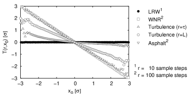
Figure 3: The conditional expectation value $T(r,x_{0})=\langle\Delta_{l}(t,r)\,|\,\xi(t)\!=\!x_{0}\rangle$ for different data sets. $T$ is shown as function of $x_{0}$ for fixed scales $r$.

As expected, we see that for the LRW there is no dependence of $T(r,x_{0})$ on $x_{0}$. In contrast, for the WNR as well as for the surface data the dependence is clear with $T(r,x_{0})=-x_{0}$. For the turbulent velocity increments it can be seen that on the small scale $\Delta r=\lambda$ the influence of $x_{0}$ on $T$ is only small, while on the large scale $\Delta r=L$ the dependence is more pronounced. This finding corresponds to Fig. 2, where for small scales [Fig. 2(b)] the conditional PDF of left-justified and centered increments were identical, while for large scales [Fig. 2(c)] a difference occurred.

V Conclusions

We found that for scale-dependent analysis of stochastic data, where the connections between different scales are investigated using increment statistics, the definition of the increment can be important, depending on the nature of the data. Apparent correlations between scales may be introduced by the left-justified increment. The importance of the increment definition varies between the ideal cases of the LRW (6), where it is nonrelevant, and the WNR (3), where it is crucial. In this case the use of left-justified increments leads to biased results for correlations between different scales. Especially, the surface measurement data we have studied require the centered definition on all accessible scales Waechter et al. (2003, 2004). For turbulent velocities this influence depends on the regarded length (or time) scale $r$. In previous publications Renner et al. (2001); Renner (2001) no significant difference between the drift and diffusion coefficients of the Fokker-Planck equation of $\Delta_{l}$ and $\Delta_{c}$ was found. This is in accordance with our findings in Fig. 2(b), where the PDF of $\Delta_{l}$ and $\Delta_{c}$ are shown to be identical for small scale differences $r_{0}-r_{1}$, and only at the integral length scale a difference occurs [see Fig. 2(c)]. Detailed consequences are currently being investigated Siefert and Peinke (2004).

The conditional expectation value $T(r,x_{0})$ allows to quantify the influence of a left-justified increment. Nevertheless, the specification of a threshold in a statistically meaningful way is still an open question.

While in this paper we used the increments (1) and (2) to demonstrate the introduction of spurious correlations, we expect that these considerations can be applied to general scale-dependent measures of complexity, such as the rms width $w_{r}(t)=\langle(\xi(t)-\bar{\xi})^{2}\rangle^{1/2}_{r}$ or wavelet functions. One could generally distinguish between measures which are orthogonal on different scales and those which are not Ort . We expect similar results for correlations between scales as demonstrated here for left-justified and centered increments.