Restricted and unrestricted Hartree-Fock approaches for addition spectrum and Hund’s rule of spherical quantum dots in a magnetic field

Abstract

The Roothaan and Pople-Nesbet approaches for real atoms are adapted to quantum dots in the presence of a magnetic field. Single-particle Gaussian basis sets are constructed, for each dot radius, under the condition of maximum overlap with the exact functions. The chemical potential, the charging energy and the total spin expected values have been calculated, and we have verified the validity of the quantum dot energy shell structure as well as the Hund rule for electronic occupation at zero magnetic field. For finite field, we have observed the violation of Hund’s rule and studied the influence of magnetic field on the closed and open energy shell configurations. We have also compared the present results with those obtained with $\mathbf{LS}$-coupling scheme for low electronic occupation numbers. We focus only on ground state properties and consider quantum dots populated up to $40$ electrons, constructed by GaAs or InSb semiconductors.

I Introduction

The influence of the spatial confinement on the physical properties, such as electronic spectra of nanostructured systems, is a topic of growing interest. Among the several kinds of confined systems one can detach low dimensional electronic gases and impurity atoms in metallic or semiconductor mesoscopic structures,jask as also atoms, ions and molecules trapped in microscopic cavities,jask ; conne ; riv ; waz ; beekman where the effects of the confinement become important when the typical quantum sizes - such as Fermi wavelength - reach the same order of magnitude as the sizes of the cavities. However, the energy spectrum of such systems is not only determined by the spatial confinement and the geometric shape, but also by environmental factors such as electric and magnetic fields. It is also defined by many-body effects as electron-electron interaction, which may even become more important than the confinement itself. In all cases, a correct description of the physical properties of the problem requires the system wavefunction to reflect, in an appropriated way, the presence of both confinement, internal and external interactions, and the corresponding boundary conditions. We should also mention the existence of other confined systems, for example, the ones constituted by phonons,fonon plasmonsplasmon or confined bosonic gases.boson

Low dimensional electronic gases are defined in semiconductor structures when the bulk translation symmetry is broken in one or more spatial dimensions, giving origin to 2D (quantum wells), 1D (quantum wires) or 0D (quantum dots) systems. In such structures, the charged carriers loose, for some interval of energy, the characteristic of being delocalized in both three spatial dimensions and become confined in regions of mesoscopic sizes inside the crystal. This fact transforms the continua energy bands into broken subbands and energy-gaps, or even into fully discrete energy states as for example in semiconductor quantum dots (QDs), which are the main type of confined system to be addressed in this work.

An important point to have in mind is that the usual charging model,11 ; 12 ; 13 ; 14 which reduces the electron-electron interaction inside the dot to a constant proportional to its electronic occupation, is able to reasonably reproduce the experimental findings for metallic dots. However, in order to obtain a more realistic description of many-particle semiconductor dots, their relatively lower electronic density makes imperative to consider the electron-electron interaction under a microscopic point of view. In strong confinement regimes, it may even be included in a perturbative scheme.

Various are the approaches that have been used to deal with many-particle QDs. Among them, one can cite charging model, correlated electron model,29 Green functions,30 Lanczos algorithm,16 Monte Carlo method,31 Hartree-Fock calculations32 ; 33 ; 34 ; 35 and density functional theory.36 It is useful to emphasize that not only the many-body effects but also the spatial symmetry (geometric confinement) become indispensable ingredients for a precise determination of quantum effects in the electronic structure of semiconductor QDs.

Among the several kinds of geometries confining a QD, maybe the most common be a two-dimensional one defined by a parabolic potential.costa ; 51 ; 52 ; 53 ; 54 Here we will consider a three-dimensional QD defined by an infinite spherical potential. The former describes QDs lithographically defined in the plane of a two-dimensional electron gas, while the latter describes QDs grown inside glass matrices. Some of the commonly studied topics in 3D QDs are the formation of energy shells in their spectra,43 the control of electronic correlations,44 the formation of Wigner molecules in the system,45 and the influence of the Coulomb interaction in their spectra.46 ; 47 In such spherically defined 3D QD, both spin and orbital angular momenta are good quantum numbers, and the many-particle eigenstates can be labelled according to the usual $\mathbf{LS}$-coupling scheme,condon where the exact analytic many-particle eigenstates are given as a sum over appropriated Slater determinants. However, in order to deal with QDs having higher occupation, the $\mathbf{LS}$-coupling is no longer appropriated. Therefore, we have chosen to use in this paper the Roothaan and Pople-Nesbet matrix formulationsszabo of the single determinant self-consistent Hartree-Fock formalism, respectively appropriated for handling closed and open shell configurations. With them, we also calculate the QD addition spectrum and show how a magnetic field is able to violate the Hund rule. Here we consider a QD populated with up to $N=40$ electrons under the presence of a magnetic field, and expand our basis in a set of properly optimized Gaussian functions. As a note one could, in principle, also include spin-orbit coupling in the model, where $L$ and $S$ would then no longer be good quantum numbers, but for an infinite spherical potential such coupling yields no contribution to the total energy of the system.

The paper is organized as follows. In section II, for completeness and in order to introduce our notation, both restricted and unrestricted formalisms are resumed. In section III we show the Hamiltonian model and discuss how both QD chemical potential and charging energy are calculated; also, we present details on how the inclusion of a magnetic field changes the previous formalisms, as well as how the Gaussian basis set is constructed. Finally, in section IV we show our results and we use section V to line up our conclusions.

II Theoretical method

The Hartree-Fock (HF) approach assumes that the $N$-electron ground state of an interacting system is given by the single Slater determinant $\left|\Psi_{0}\right\rangle=\left|\chi_{1}\chi_{2}...\chi_{a}\chi_{b}...\chi_{N-1}\chi_{N}\right\rangle$, where the set of optimized spin orbitals $\left\{\chi_{a}|a=1...N\right\}$ is obtained by the minimization of the total energy $E_{0}$ of such state,

$$E_{0}=\left\langle\Psi_{0}\right|H\left|\Psi_{0}\right\rangle=\sum_{a}h_{aa}+\frac{1}{2}\sum_{a}\sum_{b}\left[J_{ab}-K_{ab}\right]\text{,}$$ (1)

where the kinetic $h_{aa}$, direct $J_{ab}$, and exchange $K_{ab}$ contributions to $E_{0}$ are given by

$$h_{aa}=\left\langle\chi_{a}\right|h_{a}\left|\chi_{a}\right\rangle=-\frac{\hbar^{2}}{2m}\int d^{4}\mathbf{x}_{1}\chi_{a}^{\ast}(1)\left[\nabla^{2}\chi_{a}(1)\right]\text{,}$$

$$J_{ab}=\left\langle\chi_{a}\right|J_{b}\left|\chi_{a}\right\rangle=\frac{e^{2}}{\varepsilon}\int d^{4}\mathbf{x}_{1}\chi_{a}^{\ast}(1)\left[\int d^{4}\mathbf{x}_{2}\chi_{b}^{\ast}(2)\frac{1}{\left|\mathbf{r}_{1}-\mathbf{r}_{2}\right|}\chi_{b}(2)\right]\chi_{a}(1)\text{,}$$ (2)

$$K_{ab}=\left\langle\chi_{a}\right|K_{b}\left|\chi_{a}\right\rangle=\frac{e^{2}}{\varepsilon}\int d^{4}\mathbf{x}_{1}\chi_{a}^{\ast}(1)\left[\int d^{4}\mathbf{x}_{2}\chi_{b}^{\ast}(2)\frac{1}{\left|\mathbf{r}_{1}-\mathbf{r}_{2}\right|}\chi_{a}(2)\right]\chi_{b}(1)\text{,}$$

with $m$ ($\varepsilon$) being the effective electron mass (material dielectric constant), and $\nabla^{2}=r^{-2}(\partial/\partial r(r^{2}\partial/\partial r)-L^{2})$ being the Laplacian. The symbol $d^{4}\mathbf{x}$ is used in the integrals because the orbitals $\left\{\chi_{a}\right\}$ involve both spatial and spin parts. The minimization of Eq. (1) yields the self-consistent integro-differential HF equation, whose procedure in order to obtain the optimized spin orbitals can be found elsewhere;szabo it is given by $f\left|\chi_{a}\right\rangle=\varepsilon_{a}\left|\chi_{a}\right\rangle$, where the Fock operator is

$$f=h_{a}+\sum_{b}\left[J_{b}-K_{b}\right]\text{.}$$ (3)

It can be straightly verified that the application of $f$ on $\left|\chi_{a}\right\rangle$ can be obtained from Eq. (2). The ground state energy $E_{0}$ is calculated in each iteration of our code until a convergence of $10^{-9}$ eV be reached.

The above expressions are general in the sense that no supposition was taken on the spin orbitals $\left\{\chi_{a}\right\}$. Furthermore, the confinement potential $V(\mathbf{r})$ should be added to $H$, however, since we have chosen to work with an infinite spherical potential barrier, we have excluded it from our expressions.

II.1 Roothaan approach

The first supposition, which is the core of the Restricted Hartree-Fock approach (RHF), consists in assuming that both $\alpha$ (up) and $\beta$ (down) spin functions are restricted to have the same spatial function or, more specifically, $\chi_{i}(\mathbf{x})=\left\{\psi_{j}(\mathbf{r})\alpha(\omega),\psi_{j}(\mathbf{r})\beta(\omega)\right\}$. In such way, the ground state of the system becomes $\left|\Psi_{0}^{RHF}\right\rangle=\left|\psi_{1}\overline{\psi}_{1}...\psi_{a}\overline{\psi}_{a}...\psi_{N/2}\overline{\psi}_{N/2}\right\rangle$, where a spatial function with (without) upper bar labels the spin-down (spin-up) state. Therefore, within the RHF approach, the spatial orbitals $\left\{\psi_{a}|a=1...N/2\right\}$ are doubly occupied and $\left|\Psi_{0}^{RHF}\right\rangle$ represents a closed shell system having total angular momenta $J=L=S=0$. After integration over the spin degree of freedom,szabo the HF equation in the restricted formalism becomes $f\left|\psi_{a}\right\rangle=\varepsilon_{a}\left|\psi_{a}\right\rangle$, where the Fock operator is given by

$$f=h_{a}+\sum_{b}^{N/2}\left[2J_{b}-K_{b}\right]\text{,}$$ (4)

and the ground state energy becomes

$$E_{0}^{RHF}=2\sum_{a}^{N/2}h_{aa}+\sum_{a}^{N/2}\sum_{b}^{N/2}\left[2J_{ab}-K_{ab}\right]\text{.}$$ (5)

Here, $h_{aa}=\left\langle\psi_{a}\right|h_{a}\left|\psi_{a}\right\rangle$, $J_{ab}=\left\langle\psi_{a}\right|J_{b}\left|\psi_{a}\right\rangle$, and $K_{ab}=\left\langle\psi_{a}\right|K_{b}\left|\psi_{a}\right\rangle$; so, the integrations in Eq. (2) involve only spatial functions in the RHF approach.

The Roothaan formalism consists in translating the RHF equations into a matrix formulation. This is achieved by expanding the set $\left\{\psi_{i}|i=1...k\right\}$ to be minimized, in a set of known basis functions $\left\{\phi_{\nu}|\nu=1...k\right\}$,

$$\psi_{i}=\sum_{\nu}C_{\nu i}\phi_{\nu}\text{,}$$ (6)

where the spatial orbitals having $k>N/2$ are empty. Within this procedure, the coefficients $C_{\nu i}$ become the parameters to be iterated. When Eq. (6) is inserted in the closed shell HF equation ($f$ given in Eq. (4)) and multiplied from the left by $\phi_{\mu}^{\ast}(\mathbf{r})$, one obtains the Roothaan characteristic $k$ x $k$ matrix expression,

$$\mathbf{FC}=\mathbf{SC\varepsilon}\text{,}$$ (7)

where $\mathbf{S}$ is the positive defined overlap matrix between the basis functions, whose elements are

$$S_{\mu\nu}=\int d^{3}\mathbf{r}\phi_{\mu}^{\ast}(\mathbf{r})\phi_{\nu}(\mathbf{r})\text{,}$$ (8)

$\mathbf{C}$ is the matrix of the expansion coefficients $C_{\nu i}$, whose columns describe each spatial orbital $\psi_{i}$, $\mathbf{\varepsilon}$ is the diagonal matrix of the orbital energies $\varepsilon_{i}$, and $\mathbf{F}$ is the matrix of the Fock operator $f$, whose elements are

$$F_{\mu\nu}=\int d^{3}\mathbf{r}\phi_{\mu}^{\ast}(\mathbf{r})f\phi_{\nu}(\mathbf{r})\text{.}$$ (9)

In order to explicitly write the Fock matrix, it is convenient to introduce the charge density of the system. For a closed shell configuration, described by a single determinant where each spatial orbital is doubly occupied, it can be written as $\rho(\mathbf{r})=2\sum_{a}^{N/2}\left|\psi_{a}(\mathbf{r})\right|^{2}=\sum_{\mu}\sum_{\nu}P_{\mu\nu}\phi_{\mu}(\mathbf{r})\phi_{\nu}^{\ast}(\mathbf{r})$, where one defines the density matrix $\mathbf{P}$ whose elements have the form

$$P_{\mu\nu}=2\sum_{a}^{N/2}C_{\mu a}C_{\nu a}^{\ast}\text{;}$$ (10)

observe that an integration of $\rho(\mathbf{r})$ over all space yields $N$. The elements of the Fock matrix are obtained when one inserts Eq. (4) into Eq. (9) and uses Eqs. (6) and (10). After some algebra, one gets $F_{\mu\nu}=T_{\mu\nu}+G_{\mu\nu}$, where the kinetic contribution is given by

$$T_{\mu\nu}=-\frac{\hbar^{2}}{2m}\int d^{3}\mathbf{r}\phi_{\mu}^{\ast}(\mathbf{r})\left[\nabla^{2}\phi_{\nu}(\mathbf{r})\right]\text{,}$$ (11)

while the Coulomb contribution is written as

$$G_{\mu\nu} = \frac{e^{2}}{\varepsilon}\sum_{\lambda}\sum_{\sigma}P_{\lambda\sigma}\left[\int d^{3}\mathbf{r}_{1}\int d^{3}\mathbf{r}_{2}\phi_{\mu}^{\ast}(\mathbf{r}_{1})\phi_{\sigma}^{\ast}(\mathbf{r}_{2})\frac{1}{\left|\mathbf{r}_{1}-\mathbf{r}_{2}\right|}\phi_{\nu}(\mathbf{r}_{1})\phi_{\lambda}(\mathbf{r}_{2})\right.$$ (12)

$$\left.-\frac{1}{2}\int d^{3}\mathbf{r}_{1}\int d^{3}\mathbf{r}_{2}\phi_{\mu}^{\ast}(\mathbf{r}_{1})\phi_{\sigma}^{\ast}(\mathbf{r}_{2})\frac{1}{\left|\mathbf{r}_{1}-\mathbf{r}_{2}\right|}\phi_{\lambda}(\mathbf{r}_{1})\phi_{\nu}(\mathbf{r}_{2})\right]\text{.}$$

The self-consistency of this method appears as the dependence of $\mathbf{F}$ on $\mathbf{P}$ that, in turns, depends on $\mathbf{C}$, which are the parameters to be determined.

Therefore, the procedure for the solution of Eq. (7) must follow the steps: i) Given a confinement potential for the system, one specifies $N$ and $\left\{\phi_{\mu}\right\}$; ii) The integrations in $S_{\mu\nu}$ and $T_{\mu\nu}$ are done; iii) An initial guess is used for $\mathbf{P}$; iv) With $\mathbf{P}$ and the two-electron integrals one obtains the matrix $\mathbf{G}$, which is added to the matrix $\mathbf{T}$ (once calculated, this one-electron matrix no longer changes, since it does not depend on $\mathbf{P}$ or $\mathbf{C}$) to form $\mathbf{F}$; v) $\mathbf{F}$ is diagonalized in order to get $\mathbf{C}$ and $\mathbf{\varepsilon}$, and the solution is used to form a new matrix $\mathbf{P}$ from Eq. (10); vi) This iteration is performed until the desired convergence be found. The criterion for convergence may also be set in the change of the ground state energy that is calculated in each iteration; in the Roothaan formalism it can be written as

$$E_{0}^{RHF}=\frac{1}{2}\sum_{\mu}\sum_{\nu}P_{\nu\mu}\left(T_{\mu\nu}+F_{\mu\nu}\right)\text{.}$$ (13)

II.2 Pople-Nesbet approach

The second supposition is based on the relaxation of Roothaan’s restriction by letting the $\alpha$ and $\beta$ spin functions have different spatial components, which is the core of the Unrestricted Hartree-Fock approach (UHF). Thus, $\chi_{i}(\mathbf{x})=\left\{\psi_{j}^{\alpha}(\mathbf{r})\alpha(\omega),\psi_{j}^{\beta}(\mathbf{r})\beta(\omega)\right\}$, where spin-up (spin-down) electrons are described by the spatial orbitals $\left\{\psi_{j}^{\alpha}|j=1...k\right\}$ ($\{\psi_{j}^{\beta}|j=1...k\}$). Within the UHF formalism, an unrestricted wavefunction has the form $\left|\Psi^{UHF}\right\rangle=\left|\psi_{1}^{\alpha}\overline{\psi}_{1}^{\beta}...\right\rangle$, which represents an open shell system since no spatial orbital can be doubly occupied. These UHF functions are not necessarily eigenstates of the system having defined $L$ and $S$ values, and $N$ is no longer restricted to an even number, but it has to satisfy the condition $N=N^{\alpha}+N^{\beta}$, the sum of spin-up and spin-down electrons.

In analogy with the RHF case, the spin can be integrated in the UHF formalism.szabo The main difference here is that there are two coupled HF equations to be simultaneously solved. They are given by $f^{\alpha/\beta}\left|\psi_{j}^{\alpha/\beta}\right\rangle=\varepsilon_{j}^{\alpha/\beta}\left|\psi_{j}^{\alpha/\beta}\right\rangle$, where the respective Fock operators are

$$f^{\alpha/\beta}=h_{j}+\sum_{a}^{N^{\alpha/\beta}}\left[J_{a}^{\alpha/\beta}-K_{a}^{\alpha/\beta}\right]+\sum_{a}^{N^{\beta/\alpha}}J_{a}^{\beta/\alpha}\text{.}$$ (14)

Notice that this equation reduces to Eq. (4) if $\psi_{j}^{\alpha}=\psi_{j}^{\beta}$. The way in which the corresponding terms in $f^{\alpha/\beta}$ operate on $\left|\psi_{j}^{\alpha/\beta}\right\rangle$ can be obtained from Eq. (2), keeping in mind that here one deals with only spatial contributions. In both $f^{\alpha}$ and $f^{\beta}$ there is presence of a kinetic term $h_{j}$, a direct $J_{a}^{\alpha/\beta}$ and an exchange $K_{a}^{\alpha/\beta}$ term between electrons with same spin, and a direct term $J_{a}^{\beta/\alpha}$ between electrons with different spin. Observe that it is such interdependence among $f^{\alpha}$ and $\psi_{j}^{\beta}$, as well as among $f^{\beta}$ and $\psi_{j}^{\alpha}$, that makes necessary a simultaneous solution of the two HF equations in the UHF approach. Such solution yields the sets $\left\{\psi_{j}^{\alpha}\right\}$ and $\left\{\psi_{j}^{\beta}\right\}$ that minimize the ground state energy $E_{0}^{UHF}$ of the unrestricted state $\left|\Psi_{0}^{UHF}\right\rangle$, given by

$$E_{0}^{UHF}=\sum_{a}^{N^{\alpha}}h_{aa}^{\alpha}+\sum_{a}^{N^{\beta}}h_{aa}^{\beta}+\frac{1}{2}\sum_{a}^{N^{\alpha}}\sum_{b}^{N^{\alpha}}\left[J_{ab}^{\alpha\alpha}-K_{ab}^{\alpha\alpha}\right]+\frac{1}{2}\sum_{a}^{N^{\beta}}\sum_{b}^{N^{\beta}}\left[J_{ab}^{\beta\beta}-K_{ab}^{\beta\beta}\right]+\sum_{a}^{N^{\alpha}}\sum_{b}^{N^{\beta}}J_{ab}^{\alpha\beta}\text{.}$$ (15)

Here, $h_{aa}^{\alpha/\beta}=\left\langle\psi_{a}^{\alpha/\beta}\right|h_{a}\left|\psi_{a}^{\alpha/\beta}\right\rangle$, $J_{ab}^{\alpha\beta}=\left\langle\psi_{a}^{\alpha}\right|J_{b}^{\beta}\left|\psi_{a}^{\alpha}\right\rangle=\left\langle\psi_{b}^{\beta}\right|J_{a}^{\alpha}\left|\psi_{b}^{\beta}\right\rangle=J_{ba}^{\beta\alpha}$, $J_{ab}^{\alpha\alpha}=\left\langle\psi_{a}^{\alpha}\right|J_{b}^{\alpha}\left|\psi_{a}^{\alpha}\right\rangle=\left\langle\psi_{b}^{\alpha}\right|J_{a}^{\alpha}\left|\psi_{b}^{\alpha}\right\rangle=J_{ba}^{\alpha\alpha}$, plus the analog term for $J_{ab}^{\beta\beta}$. Also, $K_{ab}^{\alpha\alpha}=\left\langle\psi_{a}^{\alpha}\right|K_{b}^{\alpha}\left|\psi_{a}^{\alpha}\right\rangle=\left\langle\psi_{b}^{\alpha}\right|K_{a}^{\alpha}\left|\psi_{b}^{\alpha}\right\rangle=K_{ba}^{\alpha\alpha}$, plus the analog term for $K_{ab}^{\beta\beta}$; observe that there is no $K_{ab}^{\alpha\beta}$ term since such interaction does not exist. Furthermore, the explicit expression for each one of these integrals is straightly obtained from the spatial contributions given in Eq. (2). As should be expected, Eq. (15) reduces to Eq. (5) when $\psi_{j}^{\alpha}=\psi_{j}^{\beta}$.

The Pople-Nesbet formalism has analogy to the Roothaan one. The difference is that, instead of Eq. (6), there are two distinct expansions for the spatial orbitals $\psi^{\alpha}$ and $\psi^{\beta}$ in terms of the known basis functions $\left\{\phi_{\nu}|\nu=1...k\right\}$, given by

$$\psi_{i}^{\alpha/\beta}=\sum_{\nu}C_{\nu i}^{\alpha/\beta}\phi_{\nu}\text{.}$$ (16)

By following the same procedure as in the Roothaan matrix expressions, one obtains the two characteristic $k$ x $k$ coupled equations for the Pople-Nesbet approach,

$$\mathbf{F}^{\alpha/\beta}\mathbf{C}^{\alpha/\beta}=\mathbf{SC}^{\alpha/\beta}\mathbf{\varepsilon}^{\alpha/\beta}\text{.}$$ (17)

Here the overlap matrix $\mathbf{S}$ is defined in Eq. (8), and the meanings of $\mathbf{C}^{\alpha/\beta}$, $\mathbf{\varepsilon}^{\alpha/\beta}$, and $\mathbf{F}^{\alpha/\beta}$ become understood from the discussion following that equation. The respective Fock matrices are given by

$$F_{\mu\nu}^{\alpha/\beta}=\int d^{3}\mathbf{r}\phi_{\mu}^{\ast}(\mathbf{r})f^{\alpha/\beta}\phi_{\nu}(\mathbf{r})\text{.}$$ (18)

It is also convenient in this UHF formalism for open shell systems to introduce the charge density of the up and down spin electrons, $\rho^{\alpha/\beta}(\mathbf{r})=\sum_{a}^{N^{\alpha/\beta}}\left|\psi_{a}^{\alpha/\beta}(\mathbf{r})\right|^{2}=\sum_{\mu}\sum_{\nu}P_{\mu\nu}^{\alpha/\beta}\phi_{\mu}(\mathbf{r})\phi_{\nu}^{\ast}(\mathbf{r})$, where the elements of the corresponding density matrix for the up and down states are

$$P_{\mu\nu}^{\alpha/\beta}=\sum_{a}^{N^{\alpha/\beta}}C_{\mu a}^{\alpha/\beta}C_{\nu a}^{\alpha/\beta\ast}\text{.}$$ (19)

From these expressions one can define two new quantities. One is the total charge density, $\rho^{T}(\mathbf{r})=\rho^{\alpha}(\mathbf{r})+\rho^{\beta}(\mathbf{r})$, which yields the total number of carriers, $N$, after integrated over all space; the other is the spin density, $\rho^{S}(\mathbf{r})=\rho^{\alpha}(\mathbf{r})-\rho^{\beta}(\mathbf{r})$, whose integral over all space yields $2M_{S}$. The latter shows that unrestricted wavefunctions are eigenfunctions of $S_{Z}$, but not necessarily of $S^{2}$. Consequently, one can define the total, $\mathbf{P}^{T}$, and spin, $\mathbf{P}^{S}$, density matrices for the system as

$$\mathbf{P}^{T}=\mathbf{P}^{\alpha}+\mathbf{P}^{\beta}\text{,}$$

$$\mathbf{P}^{S}=\mathbf{P}^{\alpha}-\mathbf{P}^{\beta}\text{.}$$ (20)

Furthermore, the elements of the two Fock matrices can be obtained by inserting Eq. (14) into Eq. (18), and using Eqs. (16), (19) and (20). After some algebra, one finds $F_{\mu\nu}^{\alpha/\beta}=T_{\mu\nu}+G_{\mu\nu}^{\alpha/\beta}$, where the kinetic matrix $T_{\mu\nu}$ is defined in Eq. (11), and the two Coulomb matrices $G_{\mu\nu}^{\alpha/\beta}$ are given by

$$G_{\mu\nu}^{\alpha/\beta}=\frac{e^{2}}{\varepsilon}\sum_{\lambda}\sum_{\sigma}\left[P_{\lambda\sigma}^{T}\int d^{3}\mathbf{r}_{1}\int d^{3}\mathbf{r}_{2}\phi_{\mu}^{\ast}(\mathbf{r}_{1})\phi_{\sigma}^{\ast}(\mathbf{r}_{2})\frac{1}{\left|\mathbf{r}_{1}-\mathbf{r}_{2}\right|}\phi_{\nu}(\mathbf{r}_{1})\phi_{\lambda}(\mathbf{r}_{2})\right.$$

$$\left.-P_{\lambda\sigma}^{\alpha/\beta}\int d^{3}\mathbf{r}_{1}\int d^{3}\mathbf{r}_{2}\phi_{\mu}^{\ast}(\mathbf{r}_{1})\phi_{\sigma}^{\ast}(\mathbf{r}_{2})\frac{1}{\left|\mathbf{r}_{1}-\mathbf{r}_{2}\right|}\phi_{\lambda}(\mathbf{r}_{1})\phi_{\nu}(\mathbf{r}_{2})\right]\text{.}$$ (21)

Notice that the self-consistency again lies in the fact that both $\mathbf{F}$ matrices depend on the $\mathbf{P}$ matrices which, in turns, depend on $\mathbf{C}$ matrices. Finally, the coupling between up and down spin equations appears on the property that $\mathbf{F}^{\alpha}$ ($\mathbf{F}^{\beta}$) depends on $\mathbf{P}^{\beta}$ ($\mathbf{P}^{\alpha}$) through $\mathbf{P}^{T}$.

The procedure for the solution of Eq. (17) is the same used for Eq. (7), having in mind that now a simultaneous solution must be found for the two distinct spatial orbital sets. If the criterion for convergence in the Pople-Nesbet formalism is the ground state energy, it can be written as

$$E_{0}^{UHF}=\frac{1}{2}\sum_{\mu}\sum_{\nu}\left[P_{\nu\mu}^{T}T_{\mu\nu}+P_{\nu\mu}^{\alpha}F_{\mu\nu}^{\alpha}+P_{\nu\mu}^{\beta}F_{\mu\nu}^{\beta}\right]\text{.}$$ (22)

As already mentioned, one disadvantage of this approach is that unrestricted functions, in general, are not eigenstates of the total spin $S$, even though they have defined $S_{Z}$ values. However, one may use the expressionsszabo

$$\left\langle S^{2}\right\rangle_{UHF}=\left(\frac{N^{\alpha}-N^{\beta}}{2}\right)\left(\frac{N^{\alpha}-N^{\beta}}{2}+1\right)+N^{\beta}-\sum_{a}^{N^{\alpha}}\sum_{b}^{N^{\beta}}\left[\sum_{\mu}\sum_{\nu}C_{\mu a}^{\alpha\text{ }\ast}C_{\nu b}^{\beta}S_{\mu\nu}\right]^{2}\text{ }$$ (23)

in order to get an estimative for $S$, while $S_{Z}$ is obtained from

$$\left\langle S_{Z}\right\rangle_{UHF}=\frac{1}{2}\sum_{\mu}\sum_{\nu}\left(P_{\nu\mu}^{\alpha}-P_{\nu\mu}^{\beta}\right)S_{\mu\nu}\text{.}$$ (24)

As a last observation, the expected value of $S$ will, in general, be higher because of the contamination from other symmetries.

III Spherical quantum dot

As an application of both RHF and UHF formalisms, we consider a QD with radius $R_{0}$ confined by an infinite spherical potential in the presence of a magnetic field $\mathbf{B}=B_{0}(0,0,1)$ that can be populated up to $40$ electrons. The single-particle Hamiltonian has the form

$$H_{0}=\frac{\hbar^{2}}{2m}\left(\mathbf{k}+\frac{e}{\hbar c}\mathbf{A}\right)^{2}+g\frac{\mu_{B}}{\hbar}\mathbf{B}\cdot\mathbf{S}\text{,}$$ (25)

where $\mu_{B}=e\hbar/(2m_{0}c)$ is the Bohr magneton, $g$ is the bulk $g$-factor, and the vector potential is used in the symmetric gauge $\mathbf{A}=(\mathbf{B}\times\mathbf{r})/2$. By using the atomic units, $E_{Ry}=e^{2}/(2a_{0})$ for energy and $a_{0}=\hbar^{2}/(m_{0}e^{2})$ for length, the Hamiltonian $H_{0}$ can be written as

$$H_{0}=\frac{1}{\widetilde{m}}\frac{a_{0}^{2}}{R_{0}^{2}}\left[-\frac{1}{x^{2}}\frac{\partial}{\partial x}\left(x^{2}\frac{\partial}{\partial x}\right)+\frac{\mathbf{L}^{2}}{x^{2}}+\frac{R_{0}^{2}}{2l_{B}^{2}}\left(L_{Z}+\widetilde{m}gS_{Z}\right)+\frac{R_{0}^{4}}{4l_{B}^{4}}x^{2}\sin^{2}(\theta)\right]\text{,}$$ (26)

where $\widetilde{m}=m/m_{0}$, $l_{B}=\sqrt{\hbar c/(eB_{0})}$ is the magnetic length, and $x=r/R_{0}$ is a dimensionless variable. Without magnetic field, the normalized spatial eigenfunctions of $H_{0}$ are given by

$$\phi_{\nu}(\mathbf{r})=\phi_{n,l,m_{l}}(x,\theta,\phi)=\left[\frac{2}{R_{0}^{3}}\frac{1}{\left[j_{l+1}\left(\alpha_{nl}\right)\right]^{2}}\right]^{1/2}j_{l}\left(\alpha_{nl}x\right)Y_{l,m_{l}}(\theta,\phi)\text{.}$$ (27)

The boundary condition at the surface $r=R_{0}$ determines $\alpha_{nl}$ as the $n^{th}$ zero of the spherical Bessel function $j_{l}(\alpha_{nl}x)$; also, the spherical harmonic $Y_{l,m_{l}}(\theta,\phi)$ is the well known eigenstate of $\mathbf{L}^{2}$ and $L_{Z}$.

Table 1: Values of the five coefficients and exponents that optimize the set of Gaussians used in the expansions for the six orbitals considered in this work.

$orbital$	$V_{1},$ $D_{1}(10^{-4})$	$V_{2},$ $D_{2}(10^{-4})$	$V_{3},$ $D_{3}(10^{-4})$	$V_{4},$ $D_{4}(10^{-4})$	$V_{5},$ $D_{5}(10^{-4})$
$1s$	$0.3229,$ $0.003$	$0.2353,$ $0.328$	$0.4554,$ $0.043$	$0.9069,$ $0.330$	$0.8317,$ $0.006$
$1p$	$0.5902,$ $0.762$	$0.0646,$ $0.564$	$0.5941,$ $0.447$	$0.4599,$ $0.350$	$0.9727,$ $0.724$
$1d$	$0.7301,$ $1.120$	$0.9570,$ $0.915$	$0.8227,$ $1.620$	$0.1950,$ $0.492$	$0.4194,$ $1.100$
$2s$	$0.4823,$ $-2.260$	$0.9875,$ $-2.440$	$0.1082,$ $-1.530$	$0.4006,$ $-2.840$	$0.0342,$ $-2.260$
$1f$	$0.6377,$ $1.500$	$0.4539,$ $1.920$	$0.9730,$ $1.440$	$0.4921,$ $1.610$	$0.5498,$ $1.360$
$2p$	$0.8513,$ $-1.420$	$0.0413,$ $-3.720$	$0.0565,$ $-0.401$	$0.8797,$ $-1.410$	$0.0457,$ $-1.700$

The Hamiltonian for the electron-electron interaction, in units of $E_{Ry}$, has the form

$$H_{ee}=\frac{2}{\varepsilon}\frac{a_{0}}{R_{0}}\frac{1}{\left|\mathbf{x}_{1}-\mathbf{x}_{2}\right|}\text{.}$$ (28)

By using the multipole expansion,

$$\frac{1}{|\mathbf{x}_{1}-\mathbf{x}_{2}|}=\sum_{\kappa=0}^{\infty}\frac{4\pi}{2\kappa+1}\frac{x_{<}^{\kappa}}{x_{>}^{\kappa+1}}\sum_{m_{\kappa}=-\kappa}^{\kappa}\left(-1\right)^{m_{\kappa}}Y_{\kappa,m_{\kappa}}\left(\theta_{1},\phi_{1}\right)Y_{\kappa,-m_{\kappa}}\left(\theta_{2},\phi_{2}\right)\text{,}$$ (29)

all the angular part of the problem can be solved analytically and, after inserted into our numerical code, we are left to solve only the radial degree of freedom.

Without magnetic field, we take into account in Eqs. (6) and (16) the spatial orbitals that define the six lowest energy shells ($1s$, $1p$, $1d$, $2s$, $1f$, $2p$) under this symmetry.walecka Therefore, the index $\nu\equiv n,l,m_{l}$ can assume up to $40$ ($20$ spin-up and $20$ spin-down) possible values for the states within those shells. Certainly, the inclusion of a magnetic field lifts both spin and orbital degeneracies of those states. In our application, we shall consider two possible materials forming the QD, namely GaAs (wide-gap material) and InSb (narrow-gap material), whose defining parameters are $\widetilde{m}=0.065$, $g=0.45$ and $\varepsilon=12.65$ for GaAs, and $\widetilde{m}=0.013$, $g=-53.1$ and $\varepsilon=16.5$ for InSb.

Due to the presence of a magnetic field, some modifications on both RHF and UHF expressions must be made. In the Roothaan approach, the quadratic term in $B_{0}$ ($\sim l_{B}^{-4}$) must be added to the single-particle contribution present in $h_{aa}$ in Eq. (2), and to the matrix $T_{\mu\nu}$ in Eq. (11); the linear terms in $B_{0}$ ($\sim l_{B}^{-2}$) are zero for a closed shell configuration, thus yielding no contribution. However, all terms proportional to $B_{0}$ have to be considered in the Pople-Nesbet formalism, since we will be dealing with an open shell configuration. Both linear ($\sim B_{0}L_{Z}$) and quadratic (diamagnetic) terms can be straightly added to the definitions of $h_{aa}$ (Eq. (2)) and $T_{\mu\nu}$ (Eq. (11)). Moreover, the inclusion of the spin-dependent linear term ($\sim B_{0}S_{Z}$) in $h_{aa}$ will impose the kinetic matrix $T_{\mu\nu}$ be decomposed in its components $T_{\mu\nu}^{\alpha/\beta}$, as it occurs with $G_{\mu\nu}^{\alpha/\beta}$ in Eq. (21). Thus, under a magnetic field, we must make in the ground state energy of an unrestricted system, given in Eq. (22), the substitution $P_{\nu\mu}^{T}T_{\mu\nu}=P_{\nu\mu}^{\alpha}T_{\mu\nu}^{\alpha}+P_{\nu\mu}^{\beta}T_{\mu\nu}^{\beta}$.

Figure 1: Comparison between the expanded Gaussian basis sets used in our calculations and the respective exact spherical Bessel functions, for a GaAs QD having $N=2$ and $R_{0}=100$ Å. The left panel shows the probability densities, while the right one shows the wavefunctions. The agreement is good for all orbitals except very closed to the origin for $s$-states.

The last important detail in our approach refers to the orbital basis $\left\{\phi_{\nu}|\nu=1...k\right\}$ used in our calculations. Instead of the spherical Bessel functions of Eq. (27), the radial part of each orbital is decomposed in a sum involving five Gaussians confined to a sphere of radius $R_{0}$, while the angular part is maintained as defined by its symmetry. So, we change the basis in Eq. (27) by

$$\phi_{n,l,m_{l}}(x,\theta,\phi)=N_{nl}\left(1-x\right)^{n}x^{l}\prod_{i=1}^{n-1}\left(\widetilde{\alpha}_{il}-x\right)\sum_{k=1}^{5}V_{k}e^{-D_{k}R_{0}^{2}x^{2}}Y_{l,m_{l}}(\theta,\phi)\text{,}$$ (30)

where $N_{nl}$ is the orbital normalization, the polynomial in $\left(1-x\right)$ satisfies the boundary condition at $x=1$ ($r=R_{0}$), and the polynomial in $x$ makes the functions having $l>0$ be zero at the origin $x=0$; also, the product in $\left(\widetilde{\alpha}_{il}-x\right)$ makes the function be zero at the zeros $\widetilde{\alpha}_{il}$ of the respective spherical Bessel function transposed to the interval $0\leq x\leq 1$, and the last sum involves an expansion in five Gaussians. For $N\leq 40$, higher number of Gaussians in the expansion does not show any improvement on our results. The coefficients $V_{k}$ as well as the exponents $D_{k}$ are determined for each value of $R_{0}$, and are obtained by using the condition of maximizing the superposition between Eq. (30) and the respective spherical Bessel function. Once $V_{k}$ and $D_{k}$ are determined and the basis is found, we run our RHF (UHF) code for given values of $R_{0}$ and $N$, and find the parameters $C_{\nu i}$ ($C_{\nu i}^{\alpha/\beta}$) that better describe Eq. (6) (Eq. (16)) and give the minimal energy in Eq. (13) (Eq. (22)).

Finally, we would like to calculate two closely related quantities that give interesting information on the charging processes of a confined system. The first one is the QD chemical potential, $\mu_{dot}(N)$, which yields the energy difference between two successive ground states, and can be calculated as

$$\mu_{dot}(N)=E_{0}(N)-E_{0}(N-1)\text{.}$$ (31)

The second one is the QD charging energy, $E_{char}(N)$, which yields the energy cost for the addition of an extra electron to the system,

$$E_{char}(N)=I(N)-A(N)=E_{0}(N+1)-2E_{0}(N)+E_{0}(N-1)\text{.}$$ (32)

Here, $I(N)=E_{0}(N-1)-E_{0}(N)$ is the ionization potential, while $A(N)=E_{0}(N)-E_{0}(N+1)$ is the electronic affinity. It becomes clear, from these two equations, that $E_{char}(N)=\mu_{dot}(N+1)-\mu_{dot}(N)$.

IV Results

Figure 1 shows a comparison between the exact orbitals described by the spherical Bessel functions of Eq. (27) and the expansions involving the Gaussians of Eq. (30) used in our calculations for a GaAs QD having $N=2$ and $R_{0}=100$ Å. The right panel shows the radial wavefunctions while the left one shows the radial probability densities. Although one can observe a difference in the $s$-wavefunctions, near $x=0$, their probability densities are reasonable in that region. For any other occupation and radius, as also for InSb QDs, this same feature regarding $s$-orbitals is observed. Table 1 shows the optimized coefficients and exponents for the five Gaussians related to the six orbitals taken into account. The factor $10^{-4}$ in all exponents cancels the term $R_{0}^{2}$ in Eq. (30). Besides, all exponents related to any orbital having $n=2$ are negative since there are regions where those wavefunctions possess negative values.

In figure 2 we show results of a RHF-Roothaan calculation. In the left panel we present the ground state energy as function of the radius for a GaAs QD populated with $2$, $8$ and $18$ electrons, while the right one shows the same, but for a InSb QD populated with $2$, $34$ and $40$ electrons. These five distinct values, plus $N=20$, are the successive magic numbers for the closed shell configurations at this symmetry. In both QDs, it is noticed that the kinetic energy is much higher and totally dominates the Coulomb one at smaller radii. Thus, the energies related to different $N$ values are more distant from each other. At larger radii, or smaller electronic density, the electron-electron interaction becomes more important and the energy separation decreases. In the insets, which show a zoom at larger radii, we analyze the influence of the magnetic field on the system shell configuration. For both occupations $N$, the curves for increasing energy ordering refer to fields of $0$, $2$, $5$, $8$ and $10$ T, even though we have only labeled the cases with $N=18$ and $N=40$. For $N=2$ the presence of the magnetic field is imperceptible at those inset scales. As also expected, due to its large $g$-factor, the Zeeman splitting is much higher for the InSb QD (observe the different energy scales in the insets). Most interesting is the fact that even for a closed shell configuration, where $L=S=0$, the influence of the quadratic field (diamagnetic term) of Eq. (26, which is the only non-zero contribution in the restricted case, becomes important mainly for higher occupation numbers and fields, as well as at larger radii (notice that there are almost no difference between $0$ and $2$ T for any $N$).

Figure 2: Restricted ground state energies for a GaAs (left panel) and InSb (right panel) QD populated with $N=2$, $8$ and $18$ ($N=2$, $34$ and $40$) electrons. The Coulomb contribution is more important at larger radii. In the insets we analyze the influence of a magnetic field in the system, where one can see that even in a closed shell configuration having $L=S=0$, the presence of the field is visible due to the diamagnetic term.

In order to study spectra for any occupation we show, in figure 3, the results of a UHF-Pople-Nesbet calculation for a GaAs QD having $R_{0}=100$ Å and without magnetic field. In the left upper panel it is made a comparison between the UHF results and the non-interacting electron case, where the energy shell structure is clear for $N=2$, $8$, $18$, $20$, $34$ and $40$. Notice that the electron-electron interaction makes the energy of a QD, whose occupation corresponds to a shell less (more) than half-filled, be decreased (increased) with respect to the non-interacting case. When such occupation corresponds exactly to half-filled cases ($N=5$, $13$, $27$ and $37$), the interacting energy is approximately equal to the non-interacting one.

In the left bottom panel of figure 3 we show both QD chemical potential (left scale, Eq. (31)) and charging energy (right scale, Eq. (32)), where the respective values of $E_{0}$ are obtained from the unrestricted calculation presented in the left upper panel. Notice that $\mu_{dot}$ increases linearly as the occupation gets higher inside a given shell. When such shell is totally filled, there is an abrupt change in $\mu_{dot}$ indicating that the following shell starts its occupation; observe that the higher the occupation, the larger is the changing. An anomalous behavior seems to occur for the $2s$ shell, whose $\mu_{dot}$ value is larger than the one for the $1f$ shell (that has higher energy). The charging energy is another way to verify not only the presence of shell structure for the spectrum, but also the validity of Hund’s rule for the filling of such shells. In principle, $E_{char}$ must present larger (smaller) peaks when the total (half) occupation of a given shell is achieved; the first fact is due to the higher difficulty to the addition of an extra electron to a QD when a filled shell state is reached. The second one refers to Hund’s rule, which establishes that electrons must be added to the system with their spins being parallel, until all possible orbitals inside a given shell be occupied; this makes the total energy of the system smaller since this procedure maximizes the negative exchange contribution. However, some violations of this rule can be verified in $E_{char}$: the smaller peak of $N=27$ occurs here at $N=26$, and the larger peak of $N=20$ has a negative value.

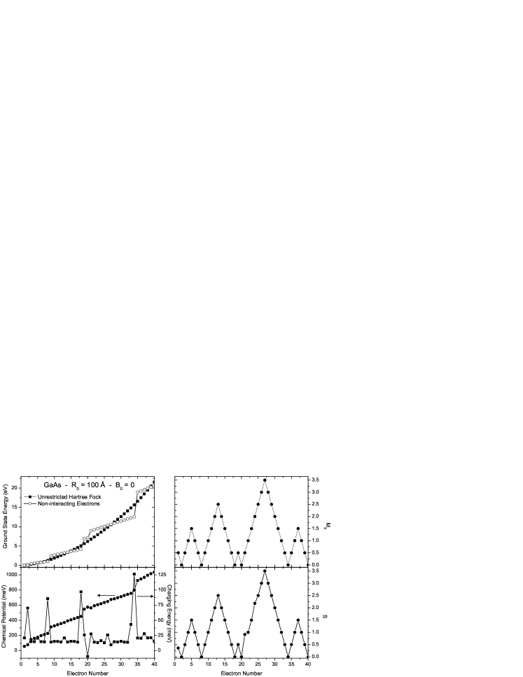
Figure 3: Unrestricted ground state energies for a $R_{0}=100$ Å GaAs QD without magnetic field. In the upper left panel we compare the unrestricted and the non-interacting energies, where the QD energy shell structure is visible. The bottom left panel shows QD chemical potential (left scale) and charging energy (right scale); the former displays abrupt change always that a new shell starts to be populated, while the latter presents larger (smaller) peaks when a shell is filled (half-filled), a direct consequence of the Hund rule. The bottom and upper right panels show, respectively, the $N$-evolution of the expected values of total spin $S$ and its projection $M_{S}$.

The bottom and upper right panels of figure 3 show respectively the evolution of the total spin $S$ and its projection $M_{S}$ as a function of QD population, calculated from Eqs. (23) and (24) for the unrestricted energies. Notice that, without magnetic field, the Hund rule seems to be followed for all states with up to 40 electrons. The $M_{S}$ expected value oscillates from $0$ in a filled shell to its maximum in a half-filled shell, when it starts to decrease again on the way to the closing of the shell; the maxima are $M_{S}=1/2$, $3/2$, $5/2$ and $7/2$ for $s$, $p$, $d$ and $f$ shells, respectively. The $S$ expected value yielded by the unrestricted formalism is also very reasonable; discrepancies are only observed at $N=24$, where $S>2$, and at $N=21$, where $S>1/2$. We believe that both discrepancies related to the $2s$ shell or to its surroundings - $\mu_{dot}$ larger than the one of $1f$ shell, negative peak for $N=20$ in $E_{char}$, and almost doubled $S$ expected value for $N=21$ - are caused by the non-reasonable Gaussian reproduction of this orbital, as visible in figure 1. These same qualitative results are observed for an InSb QD without magnetic field.

Figure 4: Violation of Hund’s rule induced by magnetic field in the $R_{0}=100$ Å GaAs QD of the previous figure. The panels show the successive occupation (indicated in the upper right corner of each panel) of the $1p$ shell, assuming that the $1s$ shell remains populated by one spin-up and one spin-down electron. The possible spin configurations for given $N$ are indicated by $+$ (spin-up) and $-$ (spin-down). For $B_{0}=0$ the spin sequence is $1/2-1-3/2-1-1/2-0$, while at fields higher than $3$ T it changes to $1/2-0-1/2-0-1/2-0$. It is interesting to observe that a magnetic field is able to suppress the energy triplets and quartets of $p$-shells from the QD spectrum.

By focusing on the $1p$ shell we show in figure 4, for the same QD of the previous figure, how a finite magnetic field is able to violate Hund’s rule in the system. Panels from left to right and from up to bottom show the successive ground state energies from $N=3$ to $N=8$ as this shell is filled, always considering that the $1s$ shell remain fully occupied by two electrons, one spin-up and one spin-down; the distinct possible spin configurations for each $N$ are indicated by $+$ (spin-up) and $-$ (spin-down). In addition to the small Zeeman effect present in all occupations, there is a change of ground state spins at $N=4$, $5$ and $6$ as the field is increased. Notice that at zero field the spin sequence is $1/2-1-3/2-1-1/2-0$; in a field above $3$ T it becomes $1/2-0-1/2-0-1/2-0$, meaning that quartets and triplets are suppressed by the magnetic field, and the ground state of the system starts to oscillate only between singlets and doublets at high fields as $N$ increases. When this $1p$ shell is half-filled ($N=5$), the ground state goes from a quartet to a doublet at $B_{0}\simeq 2$ T; when it has one electron more ($N=6$) or less ($N=4$) than that, it goes from a triplet to a singlet at $B_{0}\simeq 3$ T.

At last, we have compared the results from both RHF and UHF self-consistent matrix formulations with the ones obtained from the $\mathbf{LS}$-coupling scheme used in Ref. [LS, ], where a GaAs QD having $R_{0}=90$ Å was considered, and the quadratic term in $B_{0}$ was neglected since only small magnetic fields were considered. Also, only $N=2$ and $N=3$ occupations were calculated, since the states were constructed analytically (not only a single Slater determinant), and the electron-electron interaction was included by using perturbation theory, that is justified at such radius. At zero field the energies for $N=2$ are $16.5$ meV ($\mathbf{LS}$) and $16.1$ meV (RHF), while for $N=3$ they are $34.8$ meV ($\mathbf{LS}$) and $33.9$ meV (UHF). Therefore, both Roothaan and Pople-Nesbet formalisms indeed give smaller ground state energies than the $\mathbf{LS}$ perturbative scheme. We have also checked the validity of neglecting the diamagnetic term (quadratic in $B_{0}$) for fields smaller than $2$ T. We may emphasize here that a disadvantage of the UHF approach is, in principle, that one is never sure to get trustable information about the expected values for $L$ and $S$ in a given QD state. On the other hand, the applicability of the $\mathbf{LS}$ scheme is cumbersome and becomes very complicated to be handled analytically as the QD occupation increases.

V Conclusions

We have shown how the mean-field Roothaan and Pople-Nesbet formalisms applied to a spherical quantum dot confined system under applied magnetic field yield a fairly good description of its energy shell structure. For a maximum population of $40$ electrons considered, the appropriated Gaussian basis set for each radius has been found. We have seen how a magnetic field influences the total energy of ground states even in closed shell configurations. We have also shown how both chemical potential and charging energy reproduce the closing and half-closing structures of the quantum dot energy shells. With the calculation of the total spin expected value for each occupation, in a given radius, we have observed that Hund’s rule is satisfied at zero field. However, under finite magnetic field, we have shown that its applicability is violated and, at given values of the field, which depend on quantum dot radius and material parameters, there are transitions that change a given ground state symmetry.

- (1) W. Jaskólski, Phys. Rep. 271, 1 (1996).
- (2) J. P. Connerade, V. K. Dolmatov, P. A. Lakshmit, J. Phys. B: At. Mol. Opt. Phys. 33, 251 (2000).
- (3) R. Rivelino, J. D. M. Vianna, J. Phys. B: At. Mol. Opt. Phys. 34, L645 (2001).
- (4) D. Bielinska-Waz, J. Karkowski, G. H. F. Diercksen, J. Phys. B: At. Mol. Opt. Phys. 34, 1987 (2001).
- (5) R. A. Beekman, M. R. Roussel, P. J. Wilson, Phys. Rev. A 59, 503 (1999).
- (6) M. Grinberg, W. Jaskólski, Cz. Koepke, J. Planelles, M. Janowicz, Phys. Rev. B 50, 6504 (1994).
- (7) V. Gudmundson, R. R. Gerhardts, Phys. Rev. B 43, 12098 (1991).
- (8) M. Grossmann, M. Holthaus, Z. Phys. B 97, 319 (1995).
- (9) D. V. Averin, A. N. Korothov, K. K. Likharev, Phys. Rev. B 44, 6199 (1991).
- (10) C. W. J. Beenakker, Phys. Rev. B 44, 1646 (1991).
- (11) H. Grabert, Z. Phys. B 85, 319 (1991).
- (12) L. P. Kouwenhoven, N. C. van der Vaart, A. T. Johnson, W. Kool, C. J. P. M. Harmans, J. G. Williamson, A. A. M. Staring, C. T. Foxon, Z. Phys. B 85, 367 (1991).
- (13) D. Weinmann, W. Häusler, B. Kramer, Ann. Phys. 5, 652 (1996).
- (14) G. Cipriani, M. Rosa-Clot, S. Taddei, Phys. Rev. B 61, 7536 (2000).
- (15) K. Jauregui, W. Häusler, D. Weinmann, B. Kramer, Phys. Rev. B 53, R1713 (1996).
- (16) J. Harting, O. Mülken, P. Borrmann, Phys. Rev. B 62 , 10207 (2000).
- (17) D. Pfannkuche, V. Gudmundsson, P. A. Maksym, Phys. Rev. B 47, 2244 (1993).
- (18) Y. Alhassid, S. Malhotra, Phys. Rev. B 66, 245313 (2002).
- (19) B. Reusch, H. Grabert, Phys. Rev. B 68, 045309 (2003).
- (20) S. Bednarek, B. Szafran, J. Adamowski, Phys. Rev. B 59, 13036 (1999).
- (21) M. Ferconi, G. Vignale, Phys. Rev. B 50, 14722 (1994).
- (22) L. S. Costa, F. V. Prudente, P. H. Acioli, J. J. Soares Neto, J. D. M. Vianna, J. Phys. B: At. Mol. Opt. Phys. 32, 1 (1999).
- (23) R. C. Ashoori, H. L. Stormer, J. S. Weiner, L. N. Pfeiffer, K. W. Baldwin, K. W. West, Phys. Rev. Lett. 71, 613 (1993).
- (24) S. Tarucha, D. G. Austing, T. Honda, R. J. van der Hage, L. P. Kouwenhoven, Phys. Rev. Lett. 77, 3613 (1996).
- (25) D. J. Lockwood, P. Hawrylak, P. D. Wang, C. M. S. Torres, A. Pinczuk, B. S. Dennis, Phys. Rev. Lett. 77, 354 (1996).
- (26) P. Hawrylak, C. Gould, A. Sachradja, Y. Feng, Z. Wasilewski, Phys. Rev. B 59, 2801 (1999).
- (27) W. D. Heiss, R. G. Nazmitdinov, Phys. Rev. B 55, 16310 (1997).
- (28) Y. E. Lozovik, S. Y. Volkov, Phys. Sol. Stat. 45, 364 (2003).
- (29) P. A. Sundqvist, S. Y. Volkov, Y. E. Lozovik, M. Willander, Phys. Rev. B 66, 075335 (2002).
- (30) R. K. Pandey, M. K. Harbola, V. A. Singh, Phys. Rev. B 67, 075315 (2003).
- (31) B. Szafran, J. Adamowski, S. Bednarek, Physica E 4, 1 (1999).
- (32) E. U. Condon, G. H. Shortley, The Theory of Atomic Spectra (Cambridge University Press, London, 1977).
- (33) A. Szabo, N. S. Ostlund, Modern Quantum Chemistry: Introduction to Advanced Electronic Structure Theory (Dover, New York, 1999).
- (34) A. L. Fetter, J. D. Walecka, Quantum Theory of Many-Particle Systems (McGraw-Hill, New York, 1971).
- (35) C. F. Destefani, G. E. Marques, C. Trallero-Giner, Phys. Rev. B 65, 235314 (2002).