Abstract

In 1964, Dashen and Frautschi published two papers in the Physical Review claiming that they calculated the neutron-proton mass difference. It was once regarded as a history-making calculation, in view of the fact that the proton and neutron had been and still are regarded as the same particle with different electromagnetic properties. However, their calculation was shown to be based on a bound-state wave function which violates the localization condition in quantum mechanics.

There is one important lesson to be learned from the mistake made by Dashen and Frautschi. They did not pay much attention to the fact that there are running waves and standing waves in quantum mechanics. The S-matrix formalism is based on running waves, while bound-state problem are based on normalizable wave functions which are standing waves. Wave functions contained in the S matrix are analytic continuations of running waves, and they do not in general satisfy the localization condition for bound states.

These days, there are very serious questions raised against string theory. Is string theory a form of quantum field theory? Is it a physical theory or only a mathematical exercise. Is a new new Einstein going to emerge from string theory? It is pointed out that, if the distinction is recognized between running and standing waves, string theory has its place in the historical roadmap land-marked by Einstein, Heisenberg, Schrödinger, Dirac, Wigner, and Feynman.

1 Introduction

On April 29, at the 1965 spring meeting of the American Physical Society in Washington, Freeman Dyson of the Institute of Advanced Study (Princeton) presented an invited talk entitled “Old and New Fashions in Field Theory,” and the content of his talk was published in the June issue of the Physic Today [1]. This paper contains the following paragraph.

The first of these two achievements is the explanation of the mass difference between neutron and proton by Roger Dashen, working at the time as a graduate student under the supervision of Steve Frautschi. The neutron-proton mass difference has for thirty years been believed to be electromagnetic in origin, and it offers a splendid experimental test of any theory which tries to cover the borderline between electromagnetic and strong interactions. However, no convincing theory of the mass-difference had appeared before 1964. In this connection I exclude as unconvincing all theories, like the early theory of Feynman and Speisman, which use one arbitrary cut-off parameter to fit one experimental number. Dashen for the first time made an honest calculation without arbitrary parameters and got the right answer. His method is a beautiful marriage between old-fashioned electrodynamics and modern bootstrap techniques. He writes down the equations expressing the fact that the neutron can be considered to be a bound state of a proton with a negative pi meson, and the proton a bound state of a neutron with a positive pi meson, according to the bootstrap method. Then into these equations he puts electromagnetic perturbations, the interaction of a photon with both nucleon and pi meson, according to the Feynman rules. The calculation of the resulting mass difference is neither long nor hard to understand, and in my opinion, it will become a classic in the history of physics.

Dyson was talking about the papers by R. F. Dashen and S. C. Frautschi published in the Physical Review [2]. They use the S-matrix formalism for bound states, and then derive a formula for a perturbed energy level using the S-matrix quantities. Of course, they use approximations because they are dealing with strong interactions. There are however “good” approximations and “bad” approximations.

If we translate what they did into the language of the Schrödinger picture of quantum mechanics, Dashen and Frautschi were using the following approximation for the bound-state energy shift [3]

$$\delta E=\left(\phi^{good},\delta V\phi^{bad}\right),$$ (1)

where the good and bad bound-state wave functions are like

$$\phi^{good}\sim e^{-br},$$

$$\phi^{bad}\sim e^{br},$$ (2)

for large values of $r$, as illustrated in Fig. 1.

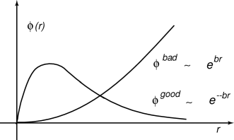
Figure 1: Good and bad wave functions contained in the S-matrix. Bound-state wave functions satisfy the localization condition and are good wave functions. Analytic continuations of plane waves do not satisfy the localization boundary condition, and become bad wave functions at the bound-state energy.

The Schrödinger equation is a second-order differential equation with two solutions. If the energy positive, there are two running-wave solutions. For negative energies, the two solutions take “good” and “bad” forms as indicated in Eq.(1). The good wave function is normalizable and carries probability interpretation. The bad wave function is not normalizable, and cannot be given any physical interpretation. If we demand that this bad wave function disappear, energy-levels become discrete. This is how the bound-state energy levels are quantized.

In the S-matrix formalism, the bound-states appear as poles in the complex energy plane. Those bound-state poles correspond to“good” localized wave functions in the Schrödinger picture. At all other places, there are unlocalized “bad” wave functions. Dashen and Frautschi overlooked this point when they used approximations in the S-matrix theory, and ended up with the “bad” formula given in Eq.(1).

Yes! Dashen and Frautschi made a serious mistake in 1964, but why do we have to raise this issue now? The answer is very simple. Since 1956, there appeared many words in physics, including dispersion relations, Mandelstam representation, Regge poles, S-matrix theory, N/D method, and bootstrap dynamics. Each of these words dominated the physics during its own period. However, they are now completely forgotten. The reason is that these temporary topics failed to place themselves to the historical roadmap.

These days, there is one domineering word in physics, particularly in particle theory. It is of course string theory. In view of the recent history, the question arises whether this theory will also be lost in history or will find its proper place in the roadmap landmarked by Einstein, Heisenberg, Schrödinger, Dirac, Wigner, and Feynman.

The purpose of string theory is to understand the physics inside relativistic particles. Since particles are localized entities in space-time, string theory necessarily has to deal with standing waves. As in the case of of the Dashen-Frautschi fiasco, it is difficult to produce standing waves within the S-matrix, or with Feynman diagrams. For standing wave problems, it would be much easier to start with standing waves.

We avoid standing waves because it is difficult to Lorentz-boost them, while it is a trivial matter to write down plane waves in a Lorentz-covariant manner. The expression for plane waves is Lorentz-invariant. Indeed, quantum field theory is possible because the plane waves are invariant. Plane waves are running waves.

Standing waves are superposition of running waves in opposite directions. Do those superpositions remain invariant under Lorentz boosts? No, but they are still covariant. This is the question we wish to exploit from the 1971 paper of Feynman, Kislinger and Ravndal [4].

In discussing standing waves, it is common to start with a hard-wall potential, but mathematically it is more comfortable to use harmonic oscillators. Indeed, in their paper of 1971, Feynman et al. start with a Lorentz-invariant harmonic oscillator equation [4]. This equation has many different solutions satisfying different boundary conditions. The solution they use is not normalizable in time-separation variable, and cannot be given any physical interpretation.

On the other hand, it is possible to fix up their mathematics. Their Lorentz-invariant differential equation has normalizable solutions which can form a representation space for Wigner’s little group for massive particles [5, 6], whose transformations leave the four-momentum of invariant. The little group dictates the internal space-time symmetry.

The normalizable oscillator solutions can be Lorentz-boosted and can be used to show that quarks and partons are two different manifestations of one covariant theory, as $E=p^{2}/2m$ and $E=cp$ are two different limits of Einstein’s energy-momentum relation.

These ingredients obtained from Feynman and Wigner could serve as the starting point for standing waves in the Lorentz-covariant world. If string theory is going to survive in history, it should find its own place in the historical raodmap. If string theory is solve the problem within a particle, it is necessarily a theory of standing waves. The issue is how to treat standing waves in Einstein’s covariant world.

In Sec. 2, we point out what Dyson says is correct but he gives a wrong example. Indeed, quantum field theory can become effective when combined with different branches of physics. We illustrate this point using the calculation of the Lamb shift.

In Sec 3, we note that there are running waves and standing waves in quantum mechanics. While it is trivial to Lorentz-boost running waves, it requires covariance of boundary conditions to understand fully standing waves. In Sec. 4, we study the S-matrix constructed from non-relativistic scattering theory. The advantage of this approach is to trace the behavior of wave functions in the S-matrix. While the bound-state in the S-matrix theory corresponds to a pole in the complex energy plane, it comes from the localization of the wave function in the Schrödinger picture. Approximations in the S-matrix does not always guarantee the localization of the bound-state wave function. This is the cause of the mistake Dashen and Frautschi made.

In Sec. 5, we review the history of bound and scattering states from comets and planets. It was Newton who observed first that the same physics is applicable to both comets and planets. Again, the same physics applies to scattering and bound states in nonrelativistic quantum mechanics. The question is what happens in Einstein’s Lorentz-covariant world. Feynman diagrams work for scattering states, but Feynman suggested the use of harmonic oscillators to approach standing-wave problems in the Lorentz-covariant world.

In Sec 6, we discuss the space-time symmetry applicable to relativistic extended particles. This symmetry is dictated by Wigner’s little group [5]. We review the progress made in this field. In Sec. 7, it is shown possible to construct the covariant harmonic oscillator wave functions. These wave functions can be Lorentz-boosted, but they depend on the time-separation variable. As a physical application of this covariant harmonic oscillator formalism,

it is shown in Sec. 8 that the quark and parton models are two different manifestation of the same covariant entity. The most controversial aspect of Feynman’s parton picture is that the partons interact incoherently with external signals. This puzzle can be explained within the framework of this oscillator formalism.

In Sec. 9, in view of Feynman’s efforts, we point out that there is a well-defined place for string theory in the Einstein’s roadmap landmarked by Heisenberg, Schrödinger, Wigner, Dirac and Feynman. String theory belongs to bound states or standing waves in the Lorentz-covariant world.

2 Lamb Shift

It is a well-accepted view that Dyson gave a wrong example for the combination of field theory and other branches of physics. Yet, Dyson was right in indicating that old-fashioned field theory could be more effective when combined with other branches of physics which produce physics which field theory cannot produce.

The Lamb-shift calculation is an excellent example. Quantum electrodynamics leads to a delta-function-like perturbing potential for the hydrogen atom. The $s-state$ wave function does not vanish at the origin while the $p-state$ does. Thus the first-order perturbation formula leads an energy shift for the $s-state$ while leaving the $p-state$ unchanged.

Of course the delta-function perturbing potential is one of the triumphs of quantum electrodynamics. On the other hand, QED cannot produce localized wave functions for the hydrogen atom. We need the Schrödinger or Dirac equation with the static coulomb potential to obtain those wave functions needed for the Lamb-shift calculation.

In order to calculate those localized bound-state wave functions, we have to impose boundary conditions at infinity. This localization condition is not properly addressed in QED or any other forms of quantum field theory.

Indeed, the wave functions used in the Lamb-shift calculation do not come from quantum field theory. Dyson was right in saying that field theory could be more effective if coupled with other branches of physics.

3 Running Waves and Standing Waves

The Dashen-Frautschi fiasco teaches us an important lesson. There are running waves and standing waves in quantum mechanics. Even though the standing wave is a superposition of running waves, it requires an additional care of boundary conditions. We do not know how to deal with this problem in the S-matrix formalism.

If not impossible, it is very difficult to formulate Lorentz boosts for rigid bodies. On the other hand, it seems to be feasible to boost waves. Indeed, quantum mechanics allows us to look at extended object as wave packets or standing waves. Thus, we are interested in boosting waves. We should note here also that there are standing and running waves.

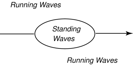
Figure 2: Running waves and standing waves in quantum theory. It a particle is allowed to travel from infinity to infinity, it corresponds to a running wave according to the wave picture of quantum mechanics. If, on the other hand, it is trapped in a localized region, we have to use standing waves to interpret its location in terms of probability distribution.

Plane waves are running waves. It is trivial to Lorentz-boost the plane wave of the form

$$\exp{\left\{i\left(\vec{p}\cdot\vec{x}-p_{0}t\right)\right\}},$$ (3)

because the exponent is invariant under Lorentz transformations. However, what would happen when different waves are superposed? Would the spectral function be covariant or invariant? What would happen for standing waves which consist of superposition of waves moving in opposite directions?

While quantum field theory based on Feynman diagrams starts with running waves, quantum mechanics within a localized space-time region deals with standing waves. If string theory is set to solve the problem inside particles, the physics of string theory is necessarily the quantum mechanics of standing waves, as is indicated in Fig. 2.

In an attempt to obtain the answers to these questions, we can start with some examples. As usual in quantum mechanics, the first example for standing waves should be a set of harmonic oscillator wave functions. With this point in mind, let us see what Feynman did for harmonic oscillators in the relativistic regime.

4 Wave Functions in S-matrix Theory

Because of the success of quantum field theory which leads to the S-matrix as the calculational tool, physicists were led to believe all the problems in physics. If this was not the case, the S-matrix should be the source of information for all physical processes.

On the other hand, the S-matrix is derivable from two fundamental theories. One is of course quantum field theory. The other is the quantum mechanics of Schrödinger and Heisenberg, which leads to non-relativistic potential scattering.

Indeed, much of the axioms or assumptions in the S-matrix theory is based on analytic properties of the S matrix in the complex energy plane. In particular, the bound state in potential scattering corresponds to a pole on in the negative energy axis. Thus, a perturbed energy-level corresponds to a displaced bound-state pole. Since the S-matrix can be formulated in a Lorentz-covariant manner, we can study the covariant picture of bound-states by studying the S-matrix poles.

On the other hand, the S-matrix in both field theory and potential scattering is basically a device to study scattering problems and is therefore formulated in terms of running waves. It does not address the localization problem of bound-state wave functions. In quantum field theory, the S-matrix cannot accommodate this localization problem because there are no localized wave functions in field theory. In potential scattering we are dealing with solutions of the Schrödinger equation which can accommodate both running and standing waves.

Let us see how we can derive the first-order energy shift for perturbed bound-state poles. We start with an attractive potential $V{r}$. For simplicity, we assume that it is spherically symmetric. Then the radial Schrödinger equation for the $\ell$th partial wave can be written as

$$\phi_{\ell}(r)=j_{\ell}(kr)+{1\over k}\int_{0}^{r}\left[n_{\ell}(kr)j_{\ell}(kr^{\prime})-j_{\ell}j(kr)n_{\ell}(kr^{\prime})\right]V_{0}(r^{\prime})\phi_{\ell}(r^{\prime})dr^{\prime},$$ (4)

where $\phi_{\ell}$ is the $\ell$th radial wave function. We define $j_{\ell}(x)$ and $n_{\ell}(x)$ as

$$j_{\ell}=\left({\pi x\over 2}\right)^{1/2}J_{\ell+{1\over 2}}(x),\qquad n_{\ell}=\left({\pi x\over 2}\right)^{1/2}N_{\ell+{1\over 2}}(x),$$ (5)

If we add a small perturbing potential $\delta V(r)$, then the perturbed wave function $\psi(r)$ satisfies the equation

$$\psi_{\ell}(r)=j_{\ell}(kr)+{1\over k}$$

$$\hskip 8.53581pt\times\int_{0}^{r}\left[n_{\ell}(kr)j_{\ell}(kr^{\prime})-j_{\ell}j(kr)n_{\ell}(kr^{\prime})\right]\left[V_{0}(r^{\prime})+\delta V(r^{\prime})\right]\psi_{\ell}(r^{\prime})dr^{\prime},$$ (6)

The perturbed wave function satisfies also the ”full-Green’s-function” integral equation:

$$\psi_{\ell}(r)=\phi_{\ell}(kr)+{1\over k}\int_{0}^{r}g_{\ell}(r,r^{\prime})\delta V_{0}(r^{\prime})\psi_{\ell}(r^{\prime})dr^{\prime},$$ (7)

which, to lowest order in $\delta V(r)$, takes the form

$$\psi_{\ell}(r)=\phi_{\ell}(kr)+{1\over k}\int_{0}^{r}g_{\ell}(r,r^{\prime})\delta V_{0}(r^{\prime})\phi_{\ell}(r^{\prime})dr^{\prime},$$ (8)

where $g_{\ell}(r^{\prime},r)$ is the “full Green’s function” constructed from the solutions of Eq.(4).

For simplicity, we now restrict ourselves to the S wave and drop the subscript $\ell$. The generalization to higher partial waves seems to be trivial. Then the integral equations in Eqs. (4), (4), and (7) take the following forms.

$$\phi(r)=j_{\ell}(kr)+{1\over k}\int_{0}^{r}\sin k(r-r^{\prime})V(r^{\prime})\phi(r^{\prime})dr^{\prime},$$

$$\psi(r)=j_{\ell}(kr)+{1\over k}\int_{0}^{r}\sin k(r-r^{\prime})[V(r^{\prime})+\delta V(r^{\prime})]\psi(r^{\prime})dr^{\prime},$$ (9)

and

$$\psi(r)=\phi(r)+{1\over k}\int_{0}^{r}g(r,r^{\prime})\delta V(r^{\prime})\phi(r^{\prime})dr^{\prime},$$ (10)

to lowest-order in $\delta V$.

In order to obtain the S matrix from the above solutions, we next introduce the Jost functions $f(\pm k)$ and $F(\pm k)$, respectively, for the perturbed and un-perturbed problems.

$$f(\pm k)=1+{1\over k}\int_{0}^{\infty}[\exp{(\mp ikr)}]V_{0}(r)\phi(r)dr,$$

$$F(\pm k)=1+{1\over k}\int_{0}^{\infty}[\exp{(\mp ikr)}]\left[V_{0}(r)+\delta V(r)\right]\psi(r)dr.$$ (11)

In terms of these Jost functions we can now write the phase shifts $\delta$ and $\eta$ for the original and perturbed problems, respectively.

$$\exp{\left(2i\delta\right)}=f(k)/f(-k),$$

$$\exp{\left(2i\eta\right)}=F(k)/F(-k).$$ (12)

Therefor, in potential scattering, we study the S-matrix in terms of the Jost functions $f(\pm k)$ or $F(\pm k)$. In the S-matrix theory, $f(k)$ is written as $N$ function or the numerator, and $f(-k)$ as the D function or the denominator. The S matrix is therefore

$$S=N/D.$$ (13)

Thus, the Jost-function approach in potential scattering corresponds to the $NoverD$ method in the S-matrix theory.

In the following discussions we will be led to study the property of the Jost functions in the complex energy plane. We thus use $s$ as the energy variable, that is,

$$s=k^{2},$$ (14)

and adopt the following notation for the Jost functions.

$$f^{(+)}(s)=f(k),\qquad F^{(+)}(s)=F(k),$$

$$f^{(-)}(s)=f(-k),\qquad F^{(-)}(s)=F(-k),$$ (15)

Let us now assume that the unperturbed problem has a bound state at $s=-s_{0}$, and therefore

$$f^{(-)}\left(-s_{0}\right)=0.$$ (16)

For the perturbed system,

$$F^{(-)}\left(-s_{0}-\delta s_{0}\right)=0,$$ (17)

where $\delta s_{0}$ is the shift in the binding energy. In order to ca1culate $\delta s_{0}$, we note from Eq.(4) that $F^{(\mp)}(s)$ can be written as

$$F^{(\mp)}(s)=f^{(\mp)}(s)+\delta f^{(\mp)}(s),$$ (18)

where

$$\delta F^{(\mp)}={1\over k}\int_{0}^{\infty}[\exp{(\pm ikr)}]V_{0}[\psi(r)-\phi(r)]dr$$

$$\hskip 28.45274pt+{1\over k}\int_{0}^{\infty}[\exp{(\pm ikr)}]\delta V\phi(r)dr.$$ (19)

If the Born approximation is valid for the unperturbed problem, both $\psi(r)$ and $\phi(r)$ become $\sin(kr)$, and $\delta f^{(\mp)}(s)$ takes the following simple form:

$$\delta F^{(\mp)}(s)={1\over k}\int_{0}^{\infty}[\exp{(\pm ikr)}]\delta V(r)\sin(kr)dr.$$ (20)

If, on the other hand, the Born approximation is not valid, we  have to use Eq. (10) for $[\psi(r)-\phi(r)]$, and the above $\delta F^{(\mp)}(s)$ becomes

$$\delta F^{(\pm)}={1\over k}\int_{0}^{\infty}[\exp{(\mp ikr)}]\delta V\phi(r)]dr$$

$$+{1\over k^{2}}\int_{0}^{\infty}[\exp{(\mp ikr)}]V(r)dr\int_{0}^{\infty}g(r,r^{\prime})\delta V\phi(r)dr.$$ (21)

We return now to the bound-state condition of Eq. (17), which can be written as

$$f^{(-)}\left(-s_{0}-\delta s_{0}\right)+F^{(-)}\left(-s_{0}-\delta s_{0}\right)=0.$$ (22)

By taking only the first-order terms in $\delta s_{0}$ and $\delta V(r)$, we arrive at the following expression for $\delta s_{0}$.

$$\delta s_{0}={\delta F^{(-)}\left(-s_{0}\right)\over\left[f^{(-)}\right]^{\prime}\left(-s_{0}\right)}$$ (23)

This is the first-order correction to the binding energy. This formula is shown to be the same as $(\phi,\delta V\phi)$ for the square-well potential where exact solutions are available for both scattering and bound states [3].

Dashen and Frautschi derived their bound-state formula from the $N/D$ method which corresponds to the above formula in non-relativistic potential scattering. In so doing, they thought they could by-pass wave functions. Furthermore, if we use the plane-wave approximation for the wave function $\phi(r)$, $\delta F^{(\pm)}$ of Eq.(4) is reduced to the Born-approximation formula of Eq.(20). It is thus tempting to use this approximation for the first try. This is precisely what Dashen and Frautschi did.

However, is the plane-wave approximation justified for bound-state problems? The plane-wave solution in this case is $sin(kr)$ in Eq.(20). When the energy becomes negative, the sine function becomes

$$\sin(kr)={1\over 2i}\left(e^{-br}-e^{br}\right),$$ (24)

where $b=\sqrt{-s_{0}}$ . For the bound state, $S_{0}$ is negative. Thus, the above wave function increases exponentially for large values of r, and is therefore a bad wave function.

What happens when we use the exact formula of Eq.(4)? The wave function $\phi(r)$ is expected to be properly localized at the energy $s=s_{0}$, and is drastically different from the bad wave function of Eq.(24).

Dashen and Frautschi made this mistake because they did not realize that there are standing waves and running waves in quantum mechanics. For present-day physics, let us see what lessons we can learn the historical mistake made by Dashen and Frautschi.

5 History of Scattering and Bound States

The issue of scattering versus bound states dates back to pre-Newton era. It was not until Newton’s second law and his law gravity that a unified view of comets and planets was established, as is illustrated in Table 1.

Table 1: History of Physics and Road Map for Strings.

		Unified
	Scattering	Physics	Bound States
Before
Newton	Comets	Unknown	Planets
Newton	Hyperbola	Newton	Ellipse
			Quantized
Bohr	Unknown	Unknown	Orbits
Quantum	Running	Particle	Standing
Mechanics	Waves	Waves	Waves
Feynman	Diagrams	Unknown	Oscillators
Future	Running Waves	One	Standing Waves
Future	* Fields	Physics	* Strings

When Bohr established the law of orbit quantization of the hydrogen atom, he was not able to explain scattering states. Then, the Schrödinger equation was able to generate scattering and bound-state solutions. The Schrödinger picture of quantum mechanics accommodates the wave nature of matter. The Schrödinger equation is a second order differential equation has two linearly independent solutions. For scattering states, it is capable of two running waves in opposite directions. For bound states, one of the solutions vanish asymptotically at infinite distance, while the other increases exponentially. We then demand that the wave function be normalizable. In this way, we give a localized probability distribution to the wave function. For scattering states, we give an interpretation of probability current.

The present form of quantum mechanics was developed for non-relativistic world. Next step is to make it consistent with Einstein’s special relativity. Since we are dealing with waves, we should learn how to Lorentz-transform waves. The question is how waves in one Lorentz frame would look to observers in different frames. The answer to this question is trivial for plane waves of the form

$$\exp{(ip\dot{x})}=\exp{\left\{i\left(\vec{p}\cdot\vec{x}-p_{0}t\right)\right\}}.$$ (25)

This form is invariant under Lorentz transformation, is usable to observers in all different Lorentz frames.

It was possible before 1950 to develop quantum field theory because field theory starts with plane waves of the form given in Eq.(25). For a superposition of plane waves:

$$\psi(x)=\int a(\vec{p})e^{ip\cdot x}d^{3}p,$$ (26)

The spectral function $a\left(\vec{p}\right)$ is defined as a covariant quantity, but it has an additional physical interpretation through second quantization or quantization of fields. Yet, the field theory starts with plane waves, and this is the reason why it is possible to develop a covariant scattering matrix. It is also possible calculate approximately the elements of this matrix using Feynman propagators based on plane waves. Feynman invented graphical approach to this procedure, and the word ”Feynman diagram” is very familiar to us.

The Feynman diagram is basically a physics of relativistic plane waves. Plane waves are running waves. How about standing waves? Here we have to take into account the fact that the standing wave consists of waves moving in two opposite directions satisfying boundary conditions. In quantum mechanics, we need those waves which can tell us about localized probability distribution in different Lorentz frames. As in the case of the hydrogen atom, the localization is defined in the three space-like dimensions. When the system is Lorentz-boosted those the longitudinal component gets mixed with the time coordinate. We do not know how to deal with this problem.

It was clear that, from the talk Feynman gave in 1970 [7], that feynman was aware of these problems. It is quite common in physics that physicists test their new theories by using harmonic oscillator, as in the case of Einstein for specific heat, Heisenberg for quantum mechanics, and Dirac for quantization of fields. Feynman boldly suggested the use of harmonic oscillator wave functions, instead of Feynman diagrams, to approach bound-state problems in Einstein’s relativistic world, as is indicates in Fig 3. Feynman talked about hadrons which are regarded as bound states of quarks. With two of his students, Feynman published a paper in the Physical Review D [4] containing the content of his paper presented at the Washington meeting. This paper contains many mathematical inconsistencies, which can be fixed up.

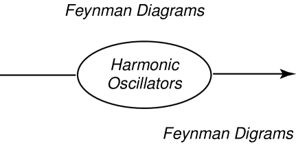
Figure 3: Feynman’s roadmap for combining quantum mechanics with special relativity. Feynman diagrams work for running waves, and they provide a satisfactory resolution for scattering states in Einstein’s world. For standing waves trapped inside an extended hadron, Feynman suggested harmonic oscillators as the first step.

Feynman et al. start with a Lorentz-invariant differential equation for the harmonic oscillator for the quarks bound together inside a hadron. For the two-quark system, they write the wave function of the form

$$\exp{\left\{{-1\over 2}\left(z^{2}-t^{2}\right)\right\}},$$ (27)

where $z$ and $t$ are the longitudinal and time-like separations between the quarks. This form is invariant under the boost, but is not normalizable in the $t$ variable. Indeed, it is a “bad” wave function as in the case of the Dashen-Frautschi fiasco.

On the other hand, the Gaussian form

$$\exp{\left\{{-1\over 2}\left(z^{2}+t^{2}\right)\right\}}$$ (28)

also satisfies Feynman’s Lorentz-invariant differential equation. This Gaussian function is normalizable, but is not invariant under the boost. However, the word “invariant” is quite different from the word “covariant.” The above form can be covariant under Lorentz transformations. We will get back to this problem in Sec. 7.

Feynman et al. studied in detail the degeneracy of the three-dimensional harmonic oscillators, and compared with the observed experimental data. Their work is complete and thorough. However, they overlooked whether their oscillator states are consistent with Wigner’s little group which governs the internal space-time symmetry of particles in Einstein’s covariant regime. They have not reached this stage.

In Sec. 6, we shall discuss see bound states or standing waves are to be constructed, and the role of Wigner’s little group for internal space-time symmetries, before discussing the covariant harmonic oscillator formalism in Sec. 7.

6 Space-time Symmetries

In solving the problems in physics, we should decide what coordinate to use. For spherical problems which are spherically symmetric, we should use spherical but not Cartesian coordinate system. For non-relativistic problems we should use Galilean coordinate system. For covariant relativistic problem, we should use Lorentz-covariant system. the problem.

Since Einstein introduced the Lorentz covariant space-time symmetry, his energy momentum relation $E=\sqrt{p^{2}+m^{2}}$ has been proven to be valid for not only point particles, but also particles with internal space-time structure, defined by quantum mechanics. Particles can have quantized spins if they are at rest of they are slowly moving. If, on the other hand, the particle is massless and moves with speed of light, it has its helicity which is the spin parallel to its momentum and gauge degree of freedom.

Table 2: Massive and massless particles in one package. Wigner’s little group unifies the internal space-time symmetries for massive and massless particles. It is a great challenge for us to find another unification: the unification of the quark and parton pictures in high-energy physics.

	Massive, Slow	COVARIANCE	Massless, Fast
Energy-		Einstein’s
Momentum	$E=p^{2}/2m$	$E=[p^{2}+m^{2}]^{1/2}$	$E=p$
Internal	$S_{3}$		$S_{3}$
Space-time		Wigner’s
Symmetry	$S_{1},S_{2}$	Little Group	Gauge Trans.
Relativistic		One
Extended	Quark Model	Covariant	Parton Model
Particles		Theory

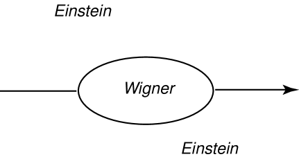
Figure 4: Wigner in Einstein’s world. Einstein formulates special relativity whose energy-momentum relation is valid for point particles as well as particles with internal space-time structure. It was Wigner who formulated the framework for internal space-time symmetries by introducing his little groups whose transformations leave the four-momentum of a given particle invariant.

Table 2 summarizes the covariant picture of the present particle world. The second row of this table indicates that the spin symmetry of slow particles and the helicity-gauge symmetry of massless particles are two limiting cases of one covariant entity called Wigner’s little group. This issue has been extensively discussed in the literature [9].

Let us then concentrate on the third row of Table 2. After Einstein formulated his special relativity, a pressing problem was to see whether his relativistic dynamics can be extended to rigid bodies as in the case of Newton’s sun and earth and their rotations. As far as we know, there are no satisfactory solutions to this problem. However, according to quantum mechanics, these extended objects are wave packets or standing waves. It might to easier to deal with waves in Einstein’s relativistic world.

Since Einstein worked with point particles when he was formulating his special relativity and did not consider the physics inside the particles, Some string theorists these days are calling for a new physics or a new Einstein applicable to internal space-time symmetry and structure of particles.

However, there also have been many respectable physicists in the past to see whether Einstein prevails inside the particles. As is illustrated in Fig. 4, Wigner formulated the concept of his little groups to deal with the internal space-time symmetry of relativistic particles.

The development of the quark model for hadrons was another important step toward understanding Einstein’s covariance. The proton is a quantum bound state of quarks. Since the proton these days can achieve a velocity very close to that of light, and is a relativistic particle in the real world.

While the proton is like a bound state when it is at rest, it appears as a collection of partons when it moves with velocity close to that of light. As we shall discuss in Sec. 8, partons have properties which appear to be quite different from those of quarks. Can we produce a standing wave solution for the proton which can explain both the quark model and the parton model?

7 Can harmonic oscillators be made covariant?

Quantum field theory has been quite successful in terms of perturbation techniques in quantum electrodynamics. However, this formalism is based on the S matrix for scattering problems and useful only for physical processes where a set of free particles becomes another set of free particles after interaction. Quantum field theory does not address the question of localized probability distributions and their covariance under Lorentz transformations. The Schrödinger quantum mechanics of the hydrogen atom deals with localized probability distribution. Indeed, the localization condition leads to the discrete energy spectrum. Here, the uncertainty relation is stated in terms of the spatial separation between the proton and the electron. If we believe in Lorentz covariance, there must also be a time-separation between the two constituent particles.

Before 1964 [8], the hydrogen atom was used for illustrating bound states. These days, we use hadrons which are bound states of quarks. Let us use the simplest hadron consisting of two quarks bound together with an attractive force, and consider their space-time positions $x_{a}$ and $x_{b}$, and use the variables

$$X=(x_{a}+x_{b})/2,\qquad x=(x_{a}-x_{b})/2\sqrt{2}.$$ (29)

The four-vector $X$ specifies where the hadron is located in space and time, while the variable $x$ measures the space-time separation between the quarks. According to Einstein, this space-time separation contains a time-like component which actively participates as can be seen from

$$\pmatrix{z^{\prime}\cr t^{\prime}}=\pmatrix{\cosh\eta&\sinh\eta\cr\sinh\eta&\cosh\eta}\pmatrix{z\cr t},$$ (30)

when the hadron is boosted along the $z$ direction. In terms of the light-cone variables defined as [10]

$$u=(z+t)/\sqrt{2},\qquad v=(z-t)/\sqrt{2},$$ (31)

the boost transformation of Eq.(30) takes the form

$$u^{\prime}=e^{\eta}u,\qquad v^{\prime}=e^{-\eta}v.$$ (32)

The $u$ variable becomes expanded while the $v$ variable becomes contracted, as is illustrated in Fig. 5.

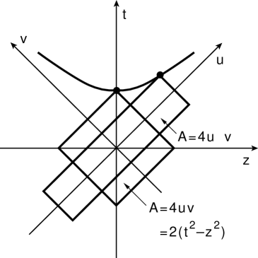
Figure 5: Lorentz boost in the light-cone coordinate system.

Does this time-separation variable exist when the hadron is at rest? Yes, according to Einstein. In the present form of quantum mechanics, we pretend not to know anything about this variable. Indeed, this variable belongs to Feynman’s rest of the universe. In this report, we shall see the role of this time-separation variable in the decoherence mechanism.

Also in the present form of quantum mechanics, there is an uncertainty relation between the time and energy variables. However, there are no known time-like excitations. Unlike Heisenberg’s uncertainty relation applicable to position and momentum, the time and energy separation variables are c-numbers, and we are not allowed to write down the commutation relation between them. Indeed, the time-energy uncertainty relation is a c-number uncertainty relation [11], as is illustrated in Fig. 6

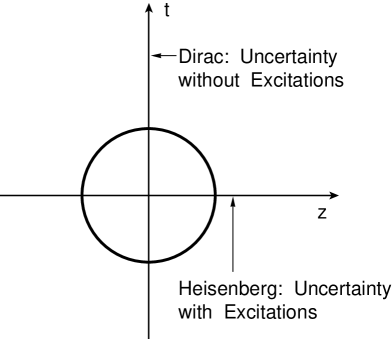
Figure 6: Space-time picture of quantum mechanics. There are quantum excitations along the space-like longitudinal direction, but there are no excitations along the time-like direction. The time-energy relation is a c-number uncertainty relation.

How does this space-time asymmetry fit into the world of covariance [12]. This question was studied in depth by the present authors in the past. The answer is that Wigner’s $O(3)$-like little group is not a Lorentz-invariant symmetry, but is a covariant symmetry [5]. It has been shown that the time-energy uncertainty applicable to the time-separation variable fits perfectly into the $O(3)$-like symmetry of massive relativistic particles [6].

The c-number time-energy uncertainty relation allows us to write down a time distribution function without excitations [6]. If we use Gaussian forms for both space and time distributions, we can start with the expression

$$\left({1\over\pi}\right)^{1/2}\exp{\left\{-{1\over 2}\left(z^{2}+t^{2}\right)\right\}}$$ (33)

for the ground-state wave function. What do Feynman et al. say about this oscillator wave function?

In their classic 1971 paper [4], Feynman et al. start with the following Lorentz-invariant differential equation.

$${1\over 2}\left\{x^{2}_{\mu}-{\partial^{2}\over\partial x_{\mu}^{2}}\right\}\psi(x)=\lambda\psi(x).$$ (34)

This partial differential equation has many different solutions depending on the choice of separable variables and boundary conditions. Feynman et al. insist on Lorentz-invariant solutions which are not normalizable. On the other hand, if we insist on normalization, the ground-state wave function takes the form of Eq.(33). It is then possible to construct a representation of the Poincaré group from the solutions of the above differential equation [6]. If the system is boosted, the wave function becomes

$$\psi_{\eta}(z,t)=\left({1\over\pi}\right)^{1/2}\exp\left\{-{1\over 2}\left(e^{-2\eta}u^{2}+e^{2\eta}v^{2}\right)\right\}.$$ (35)

This wave function becomes Eq.(33) if $\eta$ becomes zero. The transition from Eq.(33) to Eq.(35) is a squeeze transformation. The wave function of Eq.(33) is distributed within a circular region in the $uv$ plane, and thus in the $zt$ plane. On the other hand, the wave function of Eq.(35) is distributed in an elliptic region with the light-cone axes as the major and minor axes respectively. If $\eta$ becomes very large, the wave function becomes concentrated along one of the light-cone axes. Indeed, the form given in Eq.(35) is a Lorentz-squeezed wave function. This squeeze mechanism is illustrated in Fig. 7.

There are many different solutions of the Lorentz invariant differential equation of Eq.(34). The solution given in Eq.(35) is not Lorentz invariant but is covariant. It is normalizable in the $t$ variable, as well as in the space-separation variable $z$. How can we extract probability interpretation from this covariant wave function?

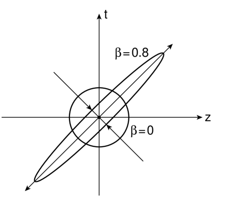
Figure 7: Effect of the Lorentz boost on the space-time wave function. The circular space-time distribution at the rest frame becomes Lorentz-squeezed to become an elliptic distribution.

8 Feynman’s Parton Picture

It is a widely accepted view that hadrons are quantum bound states of quarks having localized probability distribution. As in all bound-state cases, this localization condition is responsible for the existence of discrete mass spectra. The most convincing evidence for this bound-state picture is the hadronic mass spectra which are observed in high-energy laboratories [4, 6].

In 1969, Feynman observed that a fast-moving hadron can be regarded as a collection of many “partons” whose properties appear to be quite different from those of the quarks [13]. For example, the number of quarks inside a static proton is three, while the number of partons in a rapidly moving proton appears to be infinite. The question then is how the proton looking like a bound state of quarks to one observer can appear different to an observer in a different Lorentz frame? Feynman made the following systematic observations.

• The picture is valid only for hadrons moving with velocity close to that of light.

• The interaction time between the quarks becomes dilated, and partons behave as free independent particles.

• The momentum distribution of partons becomes widespread as the hadron moves fast.

• The number of partons seems to be infinite or much larger than that of quarks.

Because the hadron is believed to be a bound state of two or three quarks, each of the above phenomena appears as a paradox, particularly b) and c) together.

In order to resolve this paradox, let us write down the momentum-energy wave function corresponding to Eq.(35). If we let the quarks have the four-momenta $p_{a}$ and $p_{b}$, it is possible to construct two independent four-momentum variables [4]

$$P=p_{a}+p_{b},\qquad q=\sqrt{2}(p_{a}-p_{b}),$$ (36)

where $P$ is the total four-momentum. It is thus the hadronic four-momentum.

The variable $q$ measures the four-momentum separation between the quarks. Their light-cone variables are

$$q_{u}=(q_{0}-q_{z})/\sqrt{2},\qquad q_{v}=(q_{0}+q_{z})/\sqrt{2}.$$ (37)

The resulting momentum-energy wave function is

$$\phi_{\eta}(q_{z},q_{0})=\left({1\over\pi}\right)^{1/2}\exp\left\{-{1\over 2}\left(e^{-2\eta}q_{u}^{2}+e^{2\eta}q_{v}^{2}\right)\right\}.$$ (38)

Because we are using here the harmonic oscillator, the mathematical form of the above momentum-energy wave function is identical to that of the space-time wave function. The Lorentz squeeze properties of these wave functions are also the same. This aspect of the squeeze has been exhaustively discussed in the literature [6, 14, 15].

When the hadron is at rest with $\eta=0$, both wave functions behave like those for the static bound state of quarks. As $\eta$ increases, the wave functions become continuously squeezed until they become concentrated along their respective positive light-cone axes. Let us look at the z-axis projection of the space-time wave function. Indeed, the width of the quark distribution increases as the hadronic speed approaches that of the speed of light. The position of each quark appears widespread to the observer in the laboratory frame, and the quarks appear like free particles.

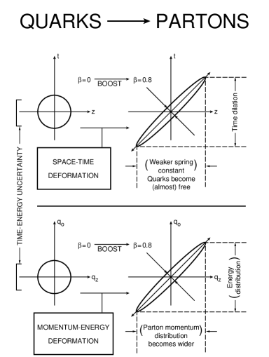
Figure 8: Lorentz-squeezed space-time and momentum-energy wave functions. As the hadron’s speed approaches that of light, both wave functions become concentrated along their respective positive light-cone axes. These light-cone concentrations lead to Feynman’s parton picture.

The momentum-energy wave function is just like the space-time wave function, as is shown in Fig. 8. The longitudinal momentum distribution becomes wide-spread as the hadronic speed approaches the velocity of light. This is in contradiction with our expectation from non-relativistic quantum mechanics that the width of the momentum distribution is inversely proportional to that of the position wave function. Our expectation is that if the quarks are free, they must have their sharply defined momenta, not a wide-spread distribution.

However, according to our Lorentz-squeezed space-time and momentum-energy wave functions, the space-time width and the momentum-energy width increase in the same direction as the hadron is boosted. This is of course an effect of Lorentz covariance. This indeed is the key to the resolution of the quark-parton paradox [6, 14].

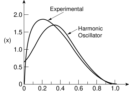
Figure 9: Parton distribution function. Theory and experiment.

After these qualitative arguments, we are interested in whether Lorentz-boosted bound-state wave functions in the hadronic rest frame could lead to parton distribution functions. If we start with the ground-state Gaussian wave function for the three-quark wave function for the proton, the parton distribution function appears as Gaussian as is indicated in Fig. 9. This Gaussian form is compared with experimental distribution also in Fig. 9.

For large $x$ region, the agreement is excellent, but the agreement is not satisfactory for small values of $x$. In this region, there is a complication called the “sea quarks.” However, good sea-quark physics starts from good valence-quark physics. Figure 9 indicates that the boosted ground-state wave function provides a good valence-quark physics.

9 Historical Destiny for Strings

Together with Marilyn Noz, the present author has been interested in question of covariant harmonic oscillators since 1973 [12]. We started with the covariant oscillator wave function as a purely phenomenological mathematical instrument. We then noticed that the covariant oscillator formalism can serve as a representation of the Wigner’s little group for massive particles, capable of the fundamental symmetry representation for relativistic particles. This allows us to deal with the c-number time-energy uncertainty relation without excitations. Furthermore, the Lorentz-boosted Gaussian wave function produces a parton distribution in satisfactory agreement with experimental data.

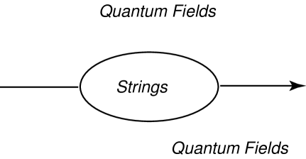
Figure 10: Roadmap for strings. If quantum fields are running waves, strings constitute the language for standing waves insider a particle localized in finite space-time region. This is the most appropriate place in Einstein’s roadmap landmarked by Wigner and Feynman.

What are then Feynman’s contributions to this subject? In addition to the formulation of the parton picture, he suggested the use of harmonic oscillator wave functions to understand bound-state problems in the covariant regime. Then where does the Feynman diagram stand in his scheme? Feynman diagrams start with plane waves which are running waves. Harmonic-oscillator wave functions are standing waves. For standing waves, we have to take care of the covariance of boundary conditions or spectral functions. This is precisely what we are reporting in this report.

It is gratifying to note that there is only one covariant quantum mechanics for both scattering and bound states. In both cases, we deal with waves in the covariant world. For scattering states, we are dealing with asymptotically free waves and Feynman diagrams. For bound states, we should start with standing waves. The covariant harmonic oscillator wave functions could constitute a complete set of wave functions we can start with.

It is our understanding that the purpose of string theory is to understand the physics inside particles, as is indicated in Fig. 10. Since particles are localized entities in the space-time region, string theory is necessarily a physics of standing waves if we are to preserve the present form of quantum mechanics. The Lorentz covariance of the standing waves should be the major issue in string theory.

References

- [1] F. J. Dyson, Physic Today 18, No. 6, 21 (1965).
- [2] R. F. Dashen and S. C. Frautschi, Phys. Rev. 135, B1190 and B1196 (1964)
- [3] Y. S. Kim, Phys. Rev. 142, 1150 (1966).
- [4] R. P. Feynman, M. Kislinger, and F. Ravndal, Phys. Rev. D 3, 2706 (1971).
- [5] E. P. Wigner, Ann. Math. 40, 149 (1939).
- [6] Y. S. Kim and M. E. Noz, Theory and Applications of the Poincaré Group (Reidel, Dordrecht, 1986).
- [7] R. P. Feynman, invited paper presented at the 1970 Washington meeting of the American Physical Society held at the Shoreham Hotel, Washington, DC, U.S.A. (April 1970).
- [8] M. Gell-Mann, Phys. Lett. 13, 598 (1964).
- [9] Y. S. Kim and E. P. Wigner, J. Math. Phys. 31, 55 (1990).
- [10] P. A. M. Dirac, Rev. Mod. Phys. 21, 392 (1949).
- [11] P. A. M. Dirac, Proc. Roy. Soc. (London) A114, 234 and 710 (1927).
- [12] Y. S. Kim and M. E. Noz, Phys. Rev. D 8, 3521 (1973).
- [13] R. P. Feynman, The Behavior of Hadron Collisions at Extreme Energies, in High Energy Collisions, Proceedings of the Third International Conference, Stony Brook, New York, edited by C. N. Yang et al., Pages 237-249 (Gordon and Breach, New York, 1969).
- [14] Y. S. Kim and M. E. Noz, Phys. Rev. D 15, 335 (1977).
- [15] Y. S. Kim, Phys. Rev. Lett. 63, 348 (1989).