Power-Law Slip Profile of the Moving Contact Line in Two-Phase Immiscible Flows

Abstract

Large scale molecular dynamics (MD) simulations on two-phase immiscible flows show that associated with the moving contact line, there is a very large $1/x$ partial-slip region where $x$ denotes the distance from the contact line. This power-law partial-slip region is verified in large-scale adaptive continuum simulations based on a local, continuum hydrodynamic formulation, which has proved successful in reproducing MD results at the nanoscale. Both MD and continuum simulations indicate the existence of a universal slip profile in the Stokes-flow regime, well described by $v^{slip}(x)/V_{w}=1/(1+{x}/{al_{s}})$, where $v^{slip}$ is the slip velocity, $V_{w}$ the speed of moving wall, $l_{s}$ the slip length, and $a$ is a numerical constant. Implications for the contact-line dissipation are discussed.

PACS: 47.11.+j, 68.08.-p, 83.10.Mj, 83.10.Ff, 83.50.Lh

Boundary condition that specifies the flow of fluid over a solid surface is a cornerstone of hydrodynamics. The no-slip condition, i.e., zero relative velocity between the fluid and solid at the interface, has been the paradigm in most of the hydrodynamics literature [1]. In molecular dynamics (MD) simulations, however, a small amount of relative slip between the fluid and the solid surface is generally detected at high flow rate [2]. Such slip can be accounted for by the Navier boundary condition (NBC), whereby the slip velocity is proportional to the tangential viscous stress [2, 3]. The proportionality constant between the slip velocity $v^{slip}$ and the shear rate is denoted the slip length $l_{s}$, usually ranging from one to a few nanometers (from MD simulations). As the amount of slip is extremely small in subsonic flow rates, the NBC is practically indistinguishable from the no-slip condition in most situations. In contrast, for immiscible flows the MD simulations have shown near-complete slip in the vicinity of the moving contact line (MCL), defined as the intersection of fluid-fluid interface with the solid wall [4, 5, 6]. An intriguing question ensues: In a mesoscopic or macroscopic system, what is the slip profile which consistently interpolates between the near complete slip at the MCL and the no-slip boundary condition that must hold at regions far away [7, 8]? Recent evidences have shown the slip profile obtained from nanoscale MD simulations to be accountable by the generalized Navier boundary condition (GNBC), in which the slip velocity is proportional to the total tangential stress — the sum of the viscous stress and the uncompensated Young stress; the latter arises from the deviation of the fluid-fluid interface from its static configuration [6]. Here we show through large-scale MD simulations and continuum hydrodynamic calculations, that there exists a power-law partial-slip region extending to hundreds of nanometers or even more, contrary to the usual expectation of a nanometer-scale slip region in the vicinity of the MCL. The existence of this large partial-slip region modifies the conventional picture that significant NBC slipping occurs only under high flow/shear rate. Instead, the power-law slip region is associated with the universal slip profile of the MCL, even at low flow rates.

MD simulations have been carried out for increasingly larger systems of immiscible Couette flow (Fig. 1). Two immiscible fluids were confined between two parallel walls in the $xy$ plane, with the fluid-solid boundaries defined by $z=0$, $H$. Periodic boundary conditions were imposed along the $x$ and $y$ directions. Interaction between fluid molecules separated by a distance $r$ was modeled by a modified Lennard-Jones (LJ) potential $U_{ff}=4\epsilon\left[\left(\sigma/r\right)^{12}-\delta_{ff}\left(\sigma/r\right)^{6}\right]$, where $\delta_{ff}=1$ for like molecules and $\delta_{ff}=-1$ for molecules of different species. The average number density for the fluids was set at $\rho=0.81/\sigma^{3}$. The temperature was controlled at $2.8\epsilon/k_{B}$. Each wall was constructed by two [001] planes of an fcc lattice, with each wall molecule attached to a lattice site by a harmonic spring. The mass of the wall molecule was set equal to that of the fluid molecule $m$. The number density of the wall was set at $\rho_{w}=1.86/\sigma^{3}$. The wall-fluid interaction was modeled by another LJ potential $U_{wf}$ with the energy and range parameters given by $\epsilon_{wf}=1.16\epsilon$ and $\sigma_{wf}=1.04\sigma$, and $\delta_{wf}$ for specifying the wetting property of the fluid, taken to be $1$ in our simulations. The Couette flow was generated by moving the top and bottom walls at a constant speed $V_{w}$ in the $\pm x$ directions, respectively. In most of our simulations, the shearing speed was $V_{w}=0.05\sqrt{\epsilon/m}$, the sample dimension along $y$ was $6.8\sigma$, the wall separation along $z$ varied from $H=6.8\sigma$ to $68\sigma$, and the sample dimension along $x$ was set to be long enough so that the uniform single-phase shear flow was recovered far away from the MCL. Steady-state interfacial and velocity profiles were obtained from time average over $5\times 10^{5}\tau$ where $\tau$ is the atomic time scale $\sqrt{m\sigma^{2}/\epsilon}$.

The tangential slip velocity profiles next to the wall, i.e., the slip profiles, are shown in the inset to Fig. 2. While there is clearly a small core region, on the order of a few $l_{s}$, where the slip profiles display sharp decay, a much more gentle variation of the slip profiles becomes apparent as the system size $H$ increases. In order to quantify the nature of the gentle variation, we plot in Fig. 2 the same data in the log-log scale. The dashed line has a slope $-1$, indicating the $1/x$ behavior to be indeed realized in MD simulations. For our finite-sized systems, there is always a plateau in the slip velocity in each of the single-phase flows, also observable in MD simulations with a value given by $v_{0}^{slip}=2V_{w}l_{s}/(H+2l_{s})$, which acts as an outer cutoff on the $1/x$ profile. This $v_{0}^{slip}$ expression is simply derived from the Navier-Stokes equation for uniform shear flow and the NBC. From our largest MD simulation, the $v^{slip}\propto 1/x$ behavior is seen to extend to $\sim 50\sigma$ (or $\sim 25l_{s}$). Hence as $H\rightarrow\infty$ and $v_{0}^{slip}$ approaches $0$ (no-slip), the power-law region can be very large indeed. A large $1/x$ partial slip region is significant, because the outer cutoff length scale directly determines the integrated effects, such as the total steady-state dissipation. While in the past the $1/x$ stress variation away from the MCL has been known [9], to our knowledge the fact that the partial slip also exhibits the same spatial dependence has not been previously seen [10], even though the validity of the Navier boundary condition at high shear stress has been verified [2, 3].

Since MD simulations reach size and accuracy (e.g., for $V_{w}/\sqrt{\epsilon/m}\ll 1$ ) limits quickly, a continuum hydrodynamic formulation is necessary for realistic simulations. In particular, continuum simulations are necessary for low flow rate immiscible flows, where MD simulations are known to be very resource intensive. Combining the GNBC with the Cahn-Hilliard (CH) hydrodynamic formulation of two-phase flow [11, 12], we have obtained a continuum hydrodynamic model [6], suitable for the calculation of much larger immiscible flows (than MD simulations) that are accurate to the molecular scale. In the same notations of Ref.[6], the continuum model is formulated as follows. The two coupled equations of motion are the Navier-Stokes (NS) equation (with the addition of the capillary force density) and the CH convection-diffusion equation for the composition field $\phi({\bf r})=(\rho_{2}-\rho_{1})/(\rho_{2}+\rho_{1})$ (where $\rho_{1}$ and $\rho_{2}$ are the local number densities for the two fluid species):

$$m\rho\left[{\partial{\bf v}\over\partial t}+\left({\bf v}\cdot\nabla\right){\bf v}\right]=-\nabla p+\nabla\cdot{\mbox{\boldmath$\sigma$}}^{v}+\mu\nabla\phi+m\rho{\bf g}_{ext},$$ (2)

$${\partial\phi\over\partial t}+{\bf v}\cdot\nabla\phi=M\nabla^{2}\mu,$$ (3)

together with the incompressibility condition $\nabla\cdot{\bf v}=0$. Here $m\rho$ is the average fluid mass density, $p$ is the pressure, ${\mbox{\boldmath$\sigma$}}^{v}$ is the Newtonian viscous stress tensor, $\mu\nabla\phi$ is the capillary force density with $\mu=\delta F/\delta\phi$ being the chemical potential defined from the CH free energy functional $F$ [13], $m\rho{\bf g}_{ext}$ is the external body force density (for Poiseuille flows), and $M$ is the phenomenological mobility coefficient. The boundary conditions at the solid surface are $v_{n}=0$, $\partial_{n}\mu=0$ ($n$ denotes the outward surface normal), the continuum form of the GNBC:

$$\beta v_{x}^{slip}=-\eta\partial_{n}v_{x}+L(\phi)\partial_{x}\phi,$$ (4)

and the relaxational equation for surface $\phi$:

$${\partial\phi\over\partial t}+{\bf v}\cdot\nabla\phi=-\Gamma L(\phi),$$ (5)

Here $L(\phi)=K\partial_{n}\phi+\partial\gamma_{wf}(\phi)/\partial\phi$ with $\gamma_{wf}(\phi)$ being the wall-fluid interfacial free energy density, $L(\phi)\partial_{x}\phi$ is the uncompensated Young stress, and $\Gamma$ is a (positive) phenomenological parameter.

The continuum results shown in Fig. 2 were calculated on a uniform mesh, using the same set of material parameters and $M$, $\Gamma$ values corresponding to the same local properties in all the five MD simulations. The overall agreement is excellent. Such agreement is possible because the GNBC does not impose an artificial cutoff on the slip region. Below we extend the MCL simulations, through continuum hydrodynamics, to lower flow rates and much larger systems.

The continuum simulation for macroscopic immiscible flows is a challenging task. Methods based on a fixed uniform mesh would break down because it cannot afford to simulate macroscopic systems with molecular resolution near the MCL. We have employed for this problem the adaptive method based on iterative grid redistribution [14]. The computational mesh is redistributed according to the behavior of the continuum solution so that fine molecular resolution is achieved in the interfacial region and near the MCL, while elsewhere a much coarser mesh is used to save computational cost. The mesh distribution is controlled by a monitor function (see [14]), and the redistribution procedure is done repeatedly as the solution evolves to its steady state. A semi-implicit time stepping scheme is also used to speed up the approach to steady state. For Couette flow, since the interface and contact line are confined in a region that is narrow in the $x$ direction but extended in the entire $z$ direction, we used a variable, adaptive grid in the $x$ direction and kept a uniform grid in the $z$ direction. This relatively simpler grid structure (compared to a general two dimensional variable grid) greatly simplifies the space discretization as well as the matrix structure in the implicit time discretization.

Figure 3 shows the continuum results for three large systems ($H$ on the order of hundreds of $\sigma$) with small $V_{w}$ ($\sim 0.001\sqrt{\epsilon/m}$, well beyond the accuracy of our MD simulations). In all three cases, the capillary force was verified to be important only in the interfacial region. In fact it decays to zero (exponentially) within a few $\sigma$. However, the pressure gradients and viscous forces shows a much slower variation. They are balanced outside the interfacial region, indicating the flow to be governed by the Stokes equation. This is expected, because the Reynolds number $m\rho V_{w}H/\eta\approx 0.6$ for $\rho\approx 0.8/\sigma^{3}$, $V_{w}=0.005\sqrt{\epsilon/m}$, $H\approx 300\sigma$, and $\eta\approx 2.0\sqrt{\epsilon m}/\sigma^{2}$. In Fig. 3 the slip profiles, plotted on the log-log scale, clearly show the $1/x$ behavior extending from $|x|\approx 6l_{s}$ to $|x|\approx 270l_{s}$. The inset to Fig. 3 shows the scaled tangential velocity profiles at the solid surface, from which the existence of universal slip profile is evident. Physically, when $H\gg l_{s}$, the regime of Stokes flow is governed by only one velocity scale $V_{w}$ and one length scale $l_{s}$. Thus universality becomes evident in terms of $v_{x}/V_{w}$ plotted as a function of $x/l_{s}$. (The inset of Fig. 2 has already shown part of the universality, that the core slip profile is independent of the system size $H$.) We give a heuristic account of the universal slip profile as follows. Away from the MCL, the viscous shear stress is given by $-a\eta v_{x}(x)/|x|$, where $a$ is a constant $\sim 1$, $\eta$ the viscosity, and $v_{x}(x)$ the local tangential velocity. The NBC implies $v_{x}^{slip}(x)=-l_{s}av_{x}(x)/|x|$. Since $v_{x}^{slip}(x)=v_{x}+V_{w}$, combining the two equations yields $v_{x}^{slip}(x)/V_{w}=1/(1+{|x|}/{al_{s}})$ [15]. This relation, with $a\approx 2.14$ for best fit, agrees with the continuum slip profiles extremely well, as seen in the inset to Fig. 3.

In the Couette geometry, external work is supplied to maintain the constant speed $V_{w}$ of the moving wall. The rate of work is given by the integral of the local tangential force $l_{s}^{-1}\eta|v^{slip}|$ times the wall speed $V_{w}$ [6], i.e.,

$$\int\left(l_{s}^{-1}\eta|v^{slip}|\right)V_{w}dx=\eta V_{w}^{2}{\cal A}$$

per unit length along $y$, where ${\cal A}$ is a numerical constant. In the limit of $V_{w}\rightarrow 0$ and $l_{s}/H\rightarrow 0$, ${\cal A}$ is independent of $V_{w}$ and $l_{s}$ but depends on the outer cutoff of the $1/x$ profile. As the external work done in the steady state must be fully dissipated, the total dissipation rate is equal to the rate of external work.

Slip profiles obtained from both MD and continuum simulations show that the $1/x$ partial-slip region starts from $x_{c}\approx 6l_{s}$ ($v^{slip}\approx 0.26V_{w}$). The outer cutoff for the partial-slip region, denoted by $R$, is determined by the overall size of the system. For the total dissipation, the contributions of the core region and the partial-slip region may be quantified by the dimensionless integrations

$${\cal A}={\cal C}=\int_{0}^{x_{c}}\left[\displaystyle\frac{|v^{slip}(x)|}{V_{w}}\right]d(\displaystyle\frac{x}{l_{s}})\approx 2.9$$

for the core and

$${\cal A}={\cal P}=\int_{x_{c}}^{R}\left[\displaystyle\frac{|v^{slip}(x)|}{V_{w}}\right]d(\displaystyle\frac{x}{l_{s}})\approx 2.14\ln\displaystyle\frac{2.14+R/l_{s}}{2.14+x_{c}/l_{s}},$$

for the $1/x$ region. Assuming $l_{s}\sim 1\;$nm (a few $\sigma$’s) [2], for $x_{c}=10\;$nm and $R=1\;\mu$m we have ${\cal P}\approx 9.2$. While for $x_{c}=10\;$nm and $R=1\;$mm we have ${\cal P}\approx 24$, i.e., the power-law region can contribute significantly more to the total dissipation than the core region.

The dissipation component that occurs at the fluid-solid interface can be evaluated as

$$\int\left(l_{s}^{-1}\eta|v^{slip}|^{2}\right)dx=\eta V_{w}^{2}{\cal I}$$

per unit length along $y$, where

$${\cal I}=\int_{0}^{R}\left[\displaystyle\frac{|v^{slip}(x)|}{V_{w}}\right]^{2}d(\displaystyle\frac{x}{l_{s}})\approx\displaystyle\frac{2.14R/l_{s}}{2.14+R/l_{s}}.$$

In the core region, the interfacial component of the dissipation is obtained by letting $R=x_{c}$, or ${\cal I}\approx 1.6$, i.e., about $70\%$ of the total interfacial dissipation (${\cal I}=2.14$ for $R/l_{s}\rightarrow\infty$).

Recently, there has been considerable interest in the transport at micro- and nanoscales. The lower limit for $R$ can reach submicrometer or even shorter length scales. On the other hand, there have been increasing evidences for large slip length realized in various fluid-solid interfaces [16, 17, 18]. Slip length $l_{s}$ as large as $1\;\mu$m has been reported [17, 18]. The results in this paper indicate that fluid-solid interfacial dissipation is an important contribution to the total dissipation if large slip length occurs in a small system. While asymptotic analysis has shown that at large distances from the MCL, the flow field is not sensitive to the slip boundary condition [19], yet the (macroscopic) asymptotic region may not be attained given the small system size and/or the large slip length. In this regard, a continuum hydrodynamic formulation of the contact-line motion is necessary for realistic simulations of fluid dynamics at micro- and nanoscales, as done in the present case.

Partial support from HKUST’s EHIA funding and Hong Kong RGC grants HKUST 6176/99P, 6143/01P, and 604803 is hereby acknowledged.

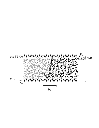
FIG. 1.: Segment of the MD simulation sample for an immiscible Couette flow with a $90^{\circ}$ static contact angle. The small empty and solid circles indicate the instantaneous molecular positions of the two fluids projected onto the $xz$ plane. The horizontally aligned black/gray circles denote the wall molecules. Between the two fluids, the large hollow circles represent the time-averaged interface profile, defined by $\rho_{1}=\rho_{2}$ ($\phi=0$). The solid line is the interface profile calculated from the continuum hydrodynamic model.

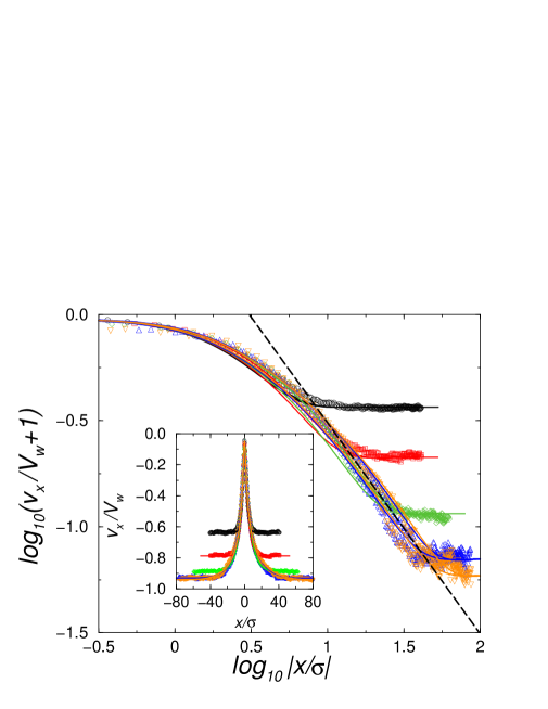
FIG. 2.: Log-log plot of the slip profiles showing the $1/x$ behavior. Here $v_{x}/V_{w}+1$ is the scaled slip velocity at the lower fluid-solid interface $z=0$, and $x/\sigma$ measures the distance from the MCL in units of $\sigma$. The wall is moving at $-V_{w}$, hence $v_{x}/V_{w}=0$ means complete slip and $v_{x}/V_{w}=-1$ means no slip. The $v_{x}$ profiles were obtained for five symmetric cases of identical wall-fluid interactions for the two fluids (both $\delta_{wf}=1$ and thus a $90^{\circ}$ static contact angle). The five cases shown here used different values for $H$ but the same value for $V_{w}$ ($=0.05\sqrt{\epsilon/m}$) and also the same parameters for densities and interactions. The symbols represent the MD results and the solid lines represent the continuum hydrodynamics results, obtained for $H=6.8\sigma$ (black circles and line), $H=13.6\sigma$ (red squares and line), $H=27.2\sigma$ (green diamonds and line), $H=54.4\sigma$ (blue up-triangles and line), $H=68\sigma$ (orange down-triangles and line). The dashed line has the slope of $-1$, indicating that the $1/x$ behavior is approached for increasingly larger $H$. For $H=68\sigma$, the $1/x$ behavior extends from $|x|\approx 12\sigma\approx 6l_{s}$ to $50\sigma\approx 25l_{s}$, where $l_{s}$ was measured to be $2\sigma$. Inset: The scaled tangential velocity $v_{x}/V_{w}$ at $z=0$ is plotted as a function of $x/\sigma$.

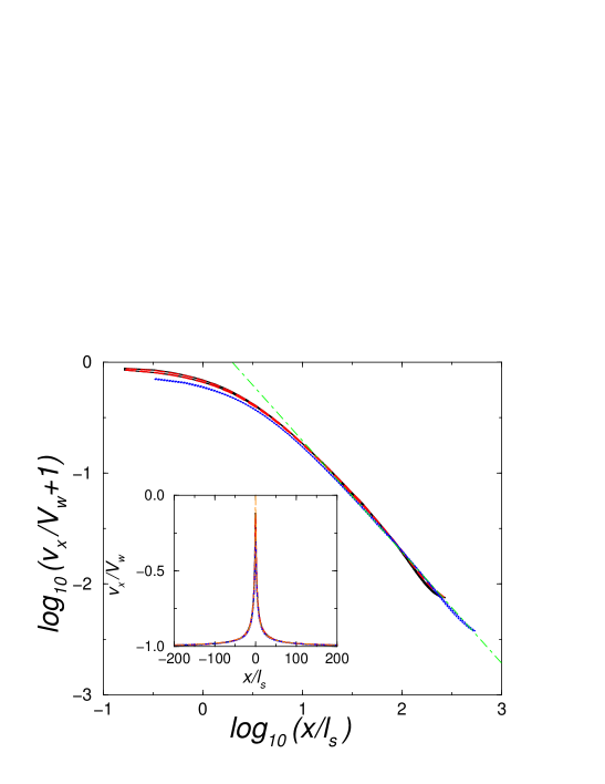
FIG. 3.: Log-log plot of the slip profiles showing the $1/x$ behavior. Here $v_{x}/V_{w}+1$ is the scaled slip velocity at the lower fluid-solid interface $z=0$, and $x/l_{s}$ measures the distance from the MCL in unit of $l_{s}$. The wall is moving at $-V_{w}$, hence $v_{x}/V_{w}=0$ means complete slip and $v_{x}/V_{w}=-1$ means no slip. The black solid line denotes the case of $H=326\sigma$, $V_{w}=0.005\sqrt{\epsilon/m}$ and $l_{s}=1.24\sigma$, the red dashed line denotes the case of $H=326\sigma$, $V_{w}=0.0025\sqrt{\epsilon/m}$ and $l_{s}=1.24\sigma$, and the blue dotted line denotes the case of $H=326\sigma$, $V_{w}=0.0025\sqrt{\epsilon/m}$ and $l_{s}=0.62\sigma$. The green dot-dashed line has the slope of $-1$, indicating a power-law region much wider than that in Fig. 2. Inset: Universal slip profile. The scaled tangential velocities $v_{x}/V_{w}$ at $z=0$ for all three cases are plotted as a function of the scaled coordinate $x/l_{s}$. It is seen that the slip profiles show a partial-slip region as large as hundreds of $l_{s}$. The relation $v_{x}/V_{w}=1/(1+{|x|}/{2.14l_{s}})-1$ is also plotted by the orange dot-dashed line, showing an extremely good fit.

REFERENCES

- [1] G. K. Batchelor, An introduction to fluid dynamics (Cambridge University Press, Cambridge, 1991).
- [2] P. A. Thompson and S. M. Troian, Nature 389, 360 (1997).
- [3] M. Cieplak, J. Koplik, and J. R. Banavar, Phys. Rev. Lett. 86, 803 (2001).
- [4] J. Koplik, J. R. Banavar, and J. F. Willemsen, Phys. Rev. Lett. 60, 1282 (1988); J. Koplik, J. R. Banavar, and J. F. Willemsen, Phys. Fluids A 1, 781 (1989).
- [5] P. A. Thompson and M. O. Robbins, Phys. Rev. Lett. 63, 766 (1989); P. A. Thompson, W. B. Brinckerhoff, and M. O. Robbins, J. Adhesion Sci. Tech. 7, 535 (1993).
- [6] T. Z. Qian, X. P. Wang, and P. Sheng, Phys. Rev. E, 68, 016306 (2003).
- [7] E. B. Dussan, V., Ann. Rev. Fluid Mech. 11, 371 (1979).
- [8] P. G. de Gennes, Rev. Mod. Phys. 57, 827 (1985).
- [9] H. K. Moffatt, J. Fluid. Mech. 18, 1 (1964); C. Hua and L. E. Scriven, J. Colloid and Interface Sci. 35, 85 (1971). The stress variation along the wall can be derived from similarity solutions for Stokes flow when a boundary velocity or stress is prescribed in the presence of a contact line or a geometric corner.
- [10] For example, an exponential slip profile was used in fitting the MD results in Ref. [5].
- [11] H. Y. Chen, D. Jasnow, and J. Vinals, Phys. Rev. Lett. 85, 1686 (2000).
- [12] D. Jacqmin, J. Fluid. Mech. 402, 57 (2000).
- [13] J. W. Cahn and J. E. Hilliard, J. Chem. Phys. 28, 258 (1958). The CH free energy functional is given by , where , and , , are parameters which can be determined in MD simulations by measuring the interface profile thickness , the interfacial tension , and the two homogeneous equilibrium phases ( in our case). See Ref. [6] for details.
- [14] W. Ren and X. P. Wang, J. Comput. Phys. 159, 246 (2000).
- [15] The similarity solution with a prescribed boundary velocity [9] becomes the leading order solution in an asymptotic expansion in the slip length , if the NBC is applied. The leading order stress variation is . As a consequence, the leading order contribution to the slip velocity is (for small ).
- [16] J-L. Barrat and L. Bocquet, Phys. Rev. Lett. 82, 4671 (1999).
- [17] D. C. Tretheway and C. D. Meinhart, Phys. Fluids 14, L9 (2002).
- [18] L. Leger, J. Phys.: Condens. Matter 15, S19 (2003).
- [19] E. B. Dussan V., J. Fluid Mech. 77, 665 (1976).