Mott scattering in strong laser fields revisited.

Abstract

In this work, we review and correct the first Born differential cross section for the process of Mott scattering of a Dirac-Volkov electron, namely, the expression (26) derived by Szymanowski et al [Physical Review A 56, 3846 (1997)]. In particular, we disagree with the expression of $\left(\frac{d\sigma}{d\Omega}\right)$ they obtained and we give the exact coefficients multiplying the various Bessel functions appearing in the scattering differential cross section. Comparison of our numerical calculations with those of Szymanowski et al. shows qualitative and quantitative differences when the incoming total electron energy and the electric field strength are increased particularly in the direction of the laser propagation. Such corrections are very important since the relativistic electronic dressing of any Dirac-Volkov charged particle gives rise to these coefficients that multiply the various Bessel functions and the relativistic study of other processes (such as excitation, ionisation, etc….) depends strongly of the correctness and reliability of the calculations for this process of Mott Scattering in presence of a laser field. Our work has been accepted [Y. Attaourti, B. Manaut, Physical Review A 68, 067401 (2003)] but only as a comment. In this paper, we give the full details of the calculations as well as the clear explanation of the large discrepancies that their results could cause when working in the ultra relativistic regime and using a very strong laser field corresponding to an electric field $\varepsilon=5.89$ in atomic units.

PACS number(s): 34.80.Qb, 12.20.Ds

1 Introduction

In a pioneering and very often cited paper , Szymanowski et al. [1] have studied the Mott scattering process in a strong laser field. The main purpose of their work was to show that the modifications of the Mott scattering differential cross section for the scattering of an electron by the Coulomb potential of a nucleus in the presence of a strong laser field, can yield interesting physical insights concerning the importance and the signatures of the relativistic effects. Their spin dependent relativistic description of Mott scattering permits to distinguish between kinematics and spin-orbit coupling effects. They have compared the results of a calculation of the first Born differential cross section for the Coulomb scattering of the Dirac-Volkov electrons dressed by a circularly polarized laser field to the first Born cross section for the Coulomb scattering of spinless Klein-Gordon particles and also to the non relativistic Schrödinger-Volkov treatment. The aim of our work is to provide the correct expression for the first-Born differential cross sections corresponding to the Coulomb scattering of the Dirac-Volkov electrons. On the one hand, we show that the terms proportional to $sin(2\phi_{0})$ are missing in [1], where $\phi_{0}$ is the phase stemming from the expression of the circularly polarized electromagnetic field. The claim of [1] that they vanish is not true. These terms do not depend on the chosen description of the circular polarization in cartesian components. On the other hand, we perform the calculations with some details and throughout this work, we use atomic units $(\hbar=e=m=1)$ where $m$ denotes the electron mass. The abbreviation DCS stands for the differential cross section.
The organization of this paper is as follows : in Section 2, we establish the expression of the $S$-matrix transition amplitude as well as the formal expression of scattering DCS. In Section 3, we give a detailed account on the various trace calculations and show that indeed there is a missing term proportional to $\sin(2\phi_{0})$ that is not equal to zero. This term as well as a term proportional to $\cos(2\phi_{0})$ contribute to $\left(\frac{d\sigma}{d\Omega}\right)$ and multiply the product $J_{s+1}(z)J_{s-1}(z)$, where $J_{s}(z)$ is an ordinary Bessel function of argument $z$ and index $s$. The argument $z$ appearing in the above mentioned product will be defined later. Then, we carry out the derivation of the correct expression of the scattering DCS associated to the exchange of a given number of laser photons. In section 4, we give some estimates of the numerical significance of our corrections. In particular, we compare numerically the Dirac-Volkov DCS we have obtained with the corresponding DCS of [1]. We end by a brief conclusion in Section 5.

2 The $S$-matrix element and the scattering differential cross section

Exact solutions of relativistic wave equations [2] are very difficult to obtain. However, in a seminal paper, Volkov [3] obtained the formal solution of the Dirac equation for the relativistic electron with 4-momentum $p^{\mu}$ inside a classical monochromatic electromagnetic field $A^{\mu}$. These solutions are called the relativistic Volkov states. The plane wave electromagnetic field $A^{\mu}$ of 4-momentum $k^{\mu}$ $(k_{\mu}k^{\mu}=k^{2}=0)$ depends only on the argument $\phi=k.x=k_{\mu}x^{\mu}$ and therefore $A^{\mu}$ is such that

$$A^{\mu}=A^{\mu}(k.x)=A^{\mu}(\phi).$$ (1)

The 4-vector $A^{\mu}$ satisfies the Lorentz gauge condition $\partial_{\mu}A^{\mu}=0$ or equivalently $k_{\mu}A^{\mu}=0$. The Dirac-Volkov equation for an electron in an external field $A_{\mu}$ is

$$\left\{(\hat{p}-\frac{1}{c}A)^{2}-c^{2}-\frac{i}{2c}F_{\mu\nu}\sigma^{\mu\nu}\right\}\psi(x)=0,$$ (2)

where $F_{\mu\nu}$ is the electromagnetic field tensor $F_{\mu\nu}=\partial_{\mu}A_{\nu}-\partial_{\nu}A_{\mu}$ and $\sigma^{\mu\nu}=\frac{1}{2}[\gamma^{\mu},\gamma^{\nu}]$. The matrices $\gamma^{\mu}$ are the anticommuting Dirac matrices such that $\gamma^{\mu}\gamma^{\nu}+\gamma^{\nu}\gamma^{\mu}=2g^{\mu\nu}1_{4}$, where $g^{\mu\nu}$ is the metric tensor $g^{\mu\nu}=diag(1,-1,-1,-1)$ and $1_{4}$ is the identity matrix in four dimensions. The solutions of Eq.(2) are the relativistic Dirac-Volkov wave functions

$$\psi_{p}(x)=R(p)\frac{u(p,s)}{\sqrt{2p_{0}V}}e^{iS(x)},$$ (3)

whith

$$R(p)=\exp{(\frac{k\!\!\!/A\!\!\!/}{2c(k.p)})}=1+\frac{k\!\!\!/A\!\!\!/}{2c(k.p)},$$ (4)

and the function $S(x)$ is given by

$$S(x)=-p.x-\int_{0}^{k.x}\frac{1}{c(k.p)}\left[p.A(\xi)-\frac{1}{2c}A^{2}(\xi)\right]d\xi.$$ (5)

In Eq.(3), $u(p,s)$ represents a Dirac bispinor which satisfies the free Dirac equation and is normalized according to $\overline{u}(p,s)u(p,s)=u^{*}(p,s)\gamma^{0}u(p,s)=2c^{2}$. We consider a circularly polarized field

$$A=a_{1}\cos(\phi)+a_{2}\sin(\phi),$$ (6)

where $\phi=k.x$. We choose $a_{1}^{2}=a_{2}^{2}=a^{2}=A^{2}$ and $a_{1}.a_{2}=a_{2}.a_{1}=0$. The Lorentz condition $k.A=0$ implies $a_{1}.k=a_{2}.k=0$. If one assumes that $A^{\mu}$ is quasi-periodic so that its time average is zero $\overline{A^{\mu}}=0$, then using the Gordon identity, the averaged 4-current is easily obtained :

$$\overline{j^{\mu}}=\frac{1}{p_{0}}\left\{p^{\mu}-\frac{1}{2c^{2}(k.p)}\overline{A^{2}}k^{\mu}\right\}.$$ (7)

If one sets

$$q^{\mu}=p^{\mu}-\frac{1}{2c^{2}(k.p)}\overline{A^{2}}k^{\mu},$$ (8)

this yields

$$q.q=q^{\mu}q_{\mu}=m_{*}^{2}c^{2},$$ (9)

with

$$m_{*}^{2}=1-\frac{\overline{A^{2}}}{c^{4}}.$$ (10)

One often calls the averaged 4-momentum $q^{\mu}$ a quasi-impulsion. Note that $q^{\mu}=(Q/c,\mathbf{q})$. The quantity $m_{*}$ plays the role of an effective mass of the electron inside the electromagnetic field. For the study of the process of Mott scattering in presence of a laser field, we use the Dirac-Volkov wave functions [3] normalized in the volume $V$:

$$\psi_{q}(x)=R(p)\frac{u(p,s)}{\sqrt{2QV}}e^{iS(q,x)},$$ (11)

whith

$$R(p) = R(q)=1+\frac{1}{2c(k.p)}k\!\!\!/A\!\!\!/$$ (12)

$$= 1+\frac{1}{2c(k.p)}(k\!\!\!/.a\!\!\!/_{1}\cos(\phi)+k\!\!\!/.a\!\!\!/_{2}\sin(\phi))$$

and

$$S(q,x) = -q.x-\frac{(a_{1}.p)}{c(k.p)}\sin(\phi)+\frac{(a_{2}.p)}{c(k.p)}\cos(\phi)$$ (13)

$$= -q.x-\frac{(a_{1}.q)}{c(k.q)}\sin(\phi)+\frac{(a_{2}.q)}{c(k.q)}\cos(\phi).$$

We turn now to the calculation of the transition amplitude. The interaction of the dressed electrons with the central Coulomb field

$$A^{\mu}=(-\frac{Z}{|\mathbf{x}|},0,0,0)$$ (14)

is considered as a first-order perturbation. This is well justified if $Z\alpha\ll 1$, where $Z$ is the nuclear charge of the nucleus considered and $\alpha$ is the fine-structure constant. We evaluate the transition matrix element for the transition ($i\rightarrow f$)

$$S_{fi}=\frac{iZ}{c}\int d^{4}x\overline{\psi}_{qf}(x)\frac{\gamma^{0}}{|\mathbf{x}|}\psi_{qi}(x).$$ (15)

We first consider the quantity

$$\overline{\psi}_{qf}(x)\frac{\gamma^{0}}{|\mathbf{x}|}\psi_{qi}(x)=\frac{1}{\sqrt{2Q_{i}V}}\frac{1}{\sqrt{2Q_{f}V}}\overline{u}(p_{f},s_{f})\overline{R}(p_{f})\frac{\gamma^{0}}{|\mathbf{x}|}R(p_{i})u(p_{i},s_{i})e^{-i(S(q_{f},x)-S(q_{i},x))}.$$ (16)

We have

$$e^{-i(S(q_{f},x)-S(q_{i},x))}=\exp[i(q_{f}-q_{i}).x-iz\sin(\phi-\phi_{0})],$$ (17)

where $z$ is such that

$$z=\sqrt{\alpha_{1}^{2}+\alpha_{2}^{2}},$$ (18)

whereas the quantities $\alpha_{1}$ and $\alpha_{2}$ are given by

$$\alpha_{1}=\frac{(a_{1}.p_{i})}{c(k.p_{i})}-\frac{(a_{1}.p_{f})}{c(k.p_{f})},\,\alpha_{2}=\frac{(a_{2}.p_{i})}{c(k.p_{i})}-\frac{(a_{2}.p_{f})}{c(k.p_{f})}$$ (19)

and the phase $\phi_{0}$ is such that $\phi_{0}=\arccos(\alpha_{1}/z)=\arcsin(\alpha_{2}/z)=\arctan(\alpha_{2}/\alpha_{1})$. It is important at this stage to perform intermediate calculations in order to reduce the numbers of $\gamma$ matrices that will appear when one calculates the scattering DCS. After some algebraic manipulations, one gets

$$\overline{u}(p_{f},s_{f})\overline{R}(p_{f})\gamma^{0}R(p_{i})u(p_{i},s_{i})$$ (20)

$$= \overline{u}(p_{f},s_{f})[C_{0}+C_{1}\cos(\phi)+C_{2}\sin(\phi)]u(p_{i},s_{i}),$$

where the three coefficients $C_{0}$, $C_{1}$ and $C_{2}$ are respectively given by

$$C_{0} = \gamma^{0}-2k_{0}a^{2}k\!\!\!/c(p_{i})c(p_{f})$$

$$C_{1} = c(p_{i})\gamma^{0}k\!\!\!/a\!\!\!/_{1}+c(p_{f})a\!\!\!/_{1}k\!\!\!/\gamma^{0}$$

$$C_{2} = c(p_{i})\gamma^{0}k\!\!\!/a\!\!\!/_{2}+c(p_{f})a\!\!\!/_{2}k\!\!\!/\gamma^{0}$$ (21)

with $c(p)=\frac{1}{2c(k.p)}$ and $k_{0}=k^{0}=\omega/c$. Therefore, the transition matrix element becomes

$$S_{fi} = \frac{iZ}{c}\int d^{4}x\frac{1}{\sqrt{2Q_{i}V}}\frac{1}{\sqrt{2Q_{f}V}}\overline{u}(p_{f},s_{f})[C_{0}+C_{1}\cos(\phi)+C_{2}\sin(\phi)]u(p_{i},s_{i})$$ (22)

$$\times \exp[i(q_{f}-q_{i}).x-izsin(\phi-\phi_{0})].$$

We now invoke the well-known identities involving ordinary Bessel functions $J_{s}(z)$

$$\left\{\begin{array}[]{c}1\\ \cos(\phi)\\ \sin(\phi)\end{array}\right\}e^{-iz\sin(\phi-\phi_{0})}=\sum_{s=-\infty}^{\infty}\left\{\begin{array}[]{c}B_{s}\\ B_{1s}\\ B_{2s}\end{array}\right\}e^{-is\phi},$$ (29)

with

$$\left\{\begin{array}[]{c}B_{s}\\ B_{1s}\\ B_{2s}\end{array}\right\}=\left\{\begin{array}[]{c}J_{s}(z)e^{is\phi_{0}}\\ (J_{s+1}(z)e^{i(s+1)\phi_{0}}+J_{s-1}(z)e^{i(s-1)\phi_{0}})/2\\ (J_{s+1}(z)e^{i(s+1)\phi_{0}}-J_{s-1}(z)e^{i(s-1)\phi_{0}})/2i\end{array}\right\}.$$ (36)

Evaluating the integrals over $x_{0}$ and $\mathbf{x}$ yields for $S_{fi}$ :

$$S_{fi}=\frac{i4\pi Z}{\sqrt{2Q_{i}V}\sqrt{2Q_{f}V}}\sum_{s=-\infty}^{\infty}\frac{2\pi\delta(Q_{f}-Q_{i}-s\omega)}{|\mathbf{q}_{f}-\mathbf{q}_{i}-s\mathbf{k}|^{2}}M_{fi}^{(s)},$$ (37)

where the quantity $M_{fi}^{(s)}$ is defined by

$$M_{fi}^{(s)}=\overline{u}(p_{f},s_{f})[C_{0}B_{s}+C_{1}B_{1s}+C_{2}B_{2s}]u(p_{i},s_{i}).$$ (38)

To evaluate the DCS, we first evaluate the transition probability per particle into final states within the range of momentum $d\mathbf{q}_{f}$

$$dW_{fi} = |S_{fi}|^{2}\frac{Vd\mathbf{q}_{f}}{(2\pi)^{3}}$$ (39)

$$= \frac{(4\pi)^{2}Z^{2}}{2Q_{i}V.2Q_{f}V}\sum_{s=-\infty}^{\infty}\frac{T2\pi\delta(Q_{f}-Q_{i}-sw)}{|\mathbf{q}_{f}-\mathbf{q}_{i}-s\mathbf{k}|^{4}}|M_{fi}^{(s)}|^{2}\frac{Vd\mathbf{q}_{f}}{(2\pi)^{3}},$$

where we have used the rule of replacement

$$[2\pi\delta(Q_{f}-Q_{i}-sw)]^{2} \rightarrow 2\pi\delta(0)2\pi\delta(Q_{f}-Q_{i}-sw)$$ (40)

$$= T2\pi\delta(Q_{f}-Q_{i}-sw).$$

Next, we have for the transition probability per unit time

$$dR_{fi} = \frac{dW_{fi}}{T}$$ (41)

$$= \frac{(4\pi)^{2}Z^{2}}{2Q_{i}V.2Q_{f}V}\sum_{s=-\infty}^{\infty}\frac{2\pi\delta(Q_{f}-Q_{i}-sw)}{|\mathbf{q}_{f}-\mathbf{q}_{i}-s\mathbf{k}|^{4}}|M_{fi}^{(s)}|^{2}\frac{Vd\mathbf{q}_{f}}{(2\pi)^{3}}.$$

Dividing $dR_{fi}$ by the flux of incoming particles

$$|\mathbf{J}^{inc}|=\frac{|\mathbf{q}_{i}|c^{2}}{Q_{i}V},$$ (42)

then using the relation $|\mathbf{q}_{f}|d|\mathbf{q}_{f}|=\frac{1}{c^{2}}Q_{f}dQ_{f}$ and integrating over the final energy, we get for the scattering DCS

$$\frac{d\sigma}{d\Omega_{f}} = \left.\frac{Z^{2}}{c^{4}}\frac{|\mathbf{q}_{f}|}{|\mathbf{q}_{i}|}\sum_{s=\-\infty}^{\infty}\frac{|M_{fi}^{(s)}|^{2}}{|\mathbf{q}_{f}-\mathbf{q}_{i}-s\mathbf{k}|^{4}}\right|_{Q_{f}=Q_{i}+sw}$$ (43)

$$= \left.\sum_{s=-\infty}^{\infty}\frac{d\sigma^{(s)}}{d\Omega_{f}}\right|_{Q_{f}=Q_{i}+sw},$$

where

$$\left.\frac{d\sigma^{(s)}}{d\Omega_{f}}\right|_{Q_{f}=Q_{i}+sw}=\left.\frac{Z^{2}}{c^{4}}\frac{|\mathbf{q}_{f}|}{|\mathbf{q}_{i}|}\frac{|M_{fi}^{(s)}|^{2}}{|\mathbf{q}_{f}-\mathbf{q}_{i}-s\mathbf{k}|^{4}}\right|_{Q_{f}=Q_{i}+sw}.$$ (44)

The calculation is now reduced to the computation of traces of $\gamma$ matrices. This is routinely done using Reduce [4]. We consider the unpolarized DCS. Therefore, the various polarization states have the same probability and the actually measured DCS is given by summing over the final polarization $s_{f}$ and averaging over the initial polarization $s_{i}$. Therefore, the unpolarized DCS is formally given by

$$\frac{d\overline{\sigma}}{d\Omega_{f}}=\left.\sum_{s=-\infty}^{\infty}\frac{d\overline{\sigma}^{(s)}}{d\Omega_{f}}\right|_{Q_{f}=Q_{i}+sw},$$ (45)

where

$$\left.\frac{d\overline{\sigma}^{(s)}}{d\Omega_{f}}\right|_{Q_{f}=Q_{i}+sw} = \frac{Z^{2}}{c^{4}}\frac{|\mathbf{q}_{f}|}{|\mathbf{q}_{i}|}\frac{1}{|\mathbf{q}_{f}-\mathbf{q}_{i}-s\mathbf{k}|^{4}}\left.\frac{1}{2}\sum_{s_{i}}\sum_{s_{f}}|M_{fi}^{(s)}|^{2}\right|_{Q_{f}=Q_{i}+sw}.$$ (46)

3 Trace calculations.

Since the controversy is very acute and precise about the results of the sum over the polarization $\frac{1}{2}\sum_{s_{i}}\sum_{s_{f}}|M_{fi}^{(s)}|^{2}$, we devote a whole section to the calculations of the various traces that intervene in the formal expression of the unpolarized DCS given by Eq.(46). We have to calculate

$$\frac{1}{2}\sum_{s_{i}}\sum_{s_{f}}|M_{fi}^{(s)}|^{2} = \frac{1}{2}\sum_{s_{i}}\sum_{s_{f}}|\overline{u}(p_{f},s_{f})[C_{0}B_{s}+C_{1}B_{1s}+C_{2}B_{2s}]u(p_{i},s_{i})|^{2}$$ (47)

$$= \frac{1}{2}\sum_{s_{i}}\sum_{s_{f}}|\overline{u}(p_{f},s_{f})\Lambda^{(s)}u(p_{i},s_{i})|^{2},$$

with

$$\Lambda^{(s)} = [\gamma^{0}-2k_{0}a^{2}k\!\!\!/c(p_{i})c(p_{f})]B_{s}$$ (48)

$$+ [c(p_{i})\gamma^{0}k\!\!\!/a\!\!\!/_{1}+c(p_{f})a\!\!\!/_{1}k\!\!\!/\gamma^{0}]B_{1s}$$

$$+ [c(p_{i})\gamma^{0}k\!\!\!/a\!\!\!/_{2}+c(p_{f})a\!\!\!/_{2}k\!\!\!/\gamma^{0}]B_{2s}.$$

Using standard techniques of the $\gamma$ matrix algebra, one has

$$\frac{1}{2}\sum_{s_{i}}\sum_{s_{f}}|M_{fi}^{(s)}|^{2}=\frac{1}{2}Tr\{(p\!\!\!/_{f}c+c^{2})\Lambda^{(s)}(p\!\!\!/_{i}c+c^{2})\overline{\Lambda}^{(s)}\},$$ (49)

with

$$\overline{\Lambda}^{(s)} = \gamma^{0}\Lambda^{(s){\dagger}}\gamma^{0}$$ (50)

$$= [\gamma^{0}-2k_{0}a^{2}k\!\!\!/c(p_{i})c(p_{f})]B^{*}_{s}$$

$$+ [c(p_{i})a\!\!\!/_{1}k\!\!\!/\gamma^{0}+c(p_{f})\gamma^{0}k\!\!\!/a\!\!\!/_{1}]B^{*}_{1s}$$

$$+ [c(p_{i})a\!\!\!/_{2}k\!\!\!/\gamma^{0}+c(p_{f})\gamma^{0}k\!\!\!/a\!\!\!/_{2}]B^{*}_{2s}.$$

There are nine main traces to be calculated. We write them explicitly

$$\mathcal{M}_{1}=Tr\{(p\!\!\!/_{f}c+c^{2})C_{0}(p\!\!\!/_{i}c+c^{2})\overline{C}_{0}\}|B_{s}|^{2},$$

$$\mathcal{M}_{2}=Tr\{(p\!\!\!/_{f}c+c^{2})C_{0}(p\!\!\!/_{i}c+c^{2})\overline{C}_{1}\}B_{s}B^{*}_{1s},$$

$$\mathcal{M}_{3}=Tr\{(p\!\!\!/_{f}c+c^{2})C_{0}(p\!\!\!/_{i}c+c^{2})\overline{C}_{2}\}B_{s}B^{*}_{2s},$$

$$\mathcal{M}_{4}=Tr\{(p\!\!\!/_{f}c+c^{2})C_{1}(p\!\!\!/_{i}c+c^{2})\overline{C}_{0}\}B^{*}_{s}B_{1s},$$

$$\mathcal{M}_{5}=Tr\{(p\!\!\!/_{f}c+c^{2})C_{1}(p\!\!\!/_{i}c+c^{2})\overline{C}_{1}\}|B_{1s}|^{2},$$ (51)

$$\mathcal{M}_{6}=Tr\{(p\!\!\!/_{f}c+c^{2})C_{1}(p\!\!\!/_{i}c+c^{2})\overline{C}_{2}\}B_{1s}B^{*}_{2s},$$

$$\mathcal{M}_{7}=Tr\{(p\!\!\!/_{f}c+c^{2})C_{2}(p\!\!\!/_{i}c+c^{2})\overline{C}_{0}\}B_{2s}B^{*}_{s},$$

$$\mathcal{M}_{8}=Tr\{(p\!\!\!/_{f}c+c^{2})C_{2}(p\!\!\!/_{i}c+c^{2})\overline{C}_{1}\}B^{*}_{1s}B_{2s},$$

$$\mathcal{M}_{9}=Tr\{(p\!\!\!/_{f}c+c^{2})C_{2}(p\!\!\!/_{i}c+c^{2})\overline{C}_{2}\}|B_{2s}|^{2}.$$

To simplify the notations, we will drop the argument of the various ordinary Bessel functions that appear. The diagonal terms give rise to

$$\left.\begin{array}[]{c}\mathcal{M}_{1}\propto|B_{s}|^{2}=J_{s}^{2},\\ \mathcal{M}_{5}\propto|B_{1s}|^{2}=\frac{1}{4}(J^{2}_{s+1}+2J_{s+1}J_{s-1}\cos(2\phi_{0})+J^{2}_{s-1}),\\ \mathcal{M}_{9}\propto|B_{2s}|^{2}=\frac{1}{4}(J^{2}_{s+1}-2J_{s+1}J_{s-1}\cos(2\phi_{0})+J^{2}_{s-1}).\end{array}\right.$$ (55)

So, taking into account the fact that the traces multiplying $|B_{s}|^{2}$, $|B_{1s}|^{2}$ and $|B_{2s}|^{2}$ are not zero, one expects that terms proportional to $J_{s+1}J_{s-1}\cos(2\phi_{0})$ will be present in the expression of the scattering DCS. The first controversy between our work and the result of Szymanowski et al [1] concerns the traces $\mathcal{M}_{6}$ and$\mathcal{M}_{8}$. Since

$$\left.\begin{array}[]{c}\mathcal{M}_{6}\propto B_{1s}B^{*}_{2s}=\frac{i}{4}(J^{2}_{s+1}-2iJ_{s+1}J_{s-1}\sin(2\phi_{0})-J^{2}_{s-1})\\ \mathcal{M}_{8}\propto B_{1s}^{*}B_{2s}=\frac{-i}{4}(J^{2}_{s+1}+2iJ_{s+1}J_{s-1}\sin(2\phi_{0})-J^{2}_{s-1})\end{array}\right.$$ (58)

and with little familiarity with the $\gamma$ matrix algebra, one can see at once that if the corresponding traces are not zero then the net contribution of $\mathcal{M}_{6}+\mathcal{M}_{8}$ will contain a term proportional to $J_{s+1}J_{s-1}\sin(2\phi_{0})$. We shall demonstrate that in what follows. We have

$$\mathcal{M}_{6} = Tr\{(p\!\!\!/_{f}c+c^{2})C_{1}(p\!\!\!/_{i}c+c^{2})\overline{C}_{2}\}B_{1s}B_{2s}^{*}$$ (59)

$$= Tr\{(p\!\!\!/_{f}c+c^{2})[c(p_{i})\gamma^{0}k\!\!\!/a\!\!\!/_{1}+c(p_{f})a\!\!\!/_{1}k\!\!\!/\gamma^{0}](p\!\!\!/_{i}c+c^{2})$$

$$[c(p_{i})a\!\!\!/_{2}k\!\!\!/\gamma^{0}+c(p_{f})\gamma^{0}k\!\!\!/a\!\!\!/_{2}]\}B_{1s}B_{2s}^{*}.$$

From now on, we define a 4-vector

$$\eta^{\mu}=(1,0,0,0).$$ (60)

We can therefore write

$$\gamma^{0}=\eta\!\!\!/.$$ (61)

Then, Eq.(59) becomes

$$\mathcal{M}_{6} = Tr\{(p\!\!\!/_{f}c+c^{2})C_{1}(p\!\!\!/_{i}c+c^{2})\overline{C}_{2}\}B_{1s}B_{2s}^{*}$$ (62)

$$= Tr\{(p\!\!\!/_{f}c+c^{2})[c(p_{i})\eta\!\!\!/k\!\!\!/a\!\!\!/_{1}+c(p_{f})a\!\!\!/_{1}k\!\!\!/\eta\!\!\!/](p\!\!\!/_{i}c+c^{2})$$

$$[c(p_{i})a\!\!\!/_{2}k\!\!\!/\eta\!\!\!/+c(p_{f})\eta\!\!\!/k\!\!\!/a\!\!\!/_{2}]\}B_{1s}B_{2s}^{*}.$$

In [1], the authors claim that the controversial $\sin(2\phi_{0})$ term disappear because it is proportional to terms like $Tr\{(p\!\!\!/_{f}c+c^{2})\gamma^{0}k\!\!\!/a\!\!\!/_{1}(p\!\!\!/_{i}c+c^{2})a\!\!\!/_{2}k\!\!\!/\gamma^{0}\}$. This term as well as $Tr\{(p\!\!\!/_{f}c+c^{2})a\!\!\!/_{1}k\!\!\!/\gamma^{0}(p\!\!\!/_{i}c+c^{2})\gamma^{0}k\!\!\!/a\!\!\!/_{2}\}$ are indeed zero but for $Tr\{(p\!\!\!/_{f}c+c^{2})\gamma^{0}k\!\!\!/a\!\!\!/_{1}(p\!\!\!/_{i}c+c^{2})\gamma^{0}k\!\!\!/a\!\!\!/_{2}\}$ and $Tr\{(p\!\!\!/_{f}c+c^{2})a\!\!\!/_{1}k\!\!\!/\gamma^{0}(p\!\!\!/_{i}c+c^{2})a\!\!\!/_{2}k\!\!\!/\gamma^{0}\}$ this is no longer true. These terms are not zero and we give explicitly their values

$$Tr\{(p\!\!\!/_{f}c+c^{2})\gamma^{0}k\!\!\!/a\!\!\!/_{1}(p\!\!\!/_{i}c+c^{2})\gamma^{0}k\!\!\!/a\!\!\!/_{2}\} = Tr\{(p\!\!\!/_{f}c+c^{2})a\!\!\!/_{1}k\!\!\!/\gamma^{0}(p\!\!\!/_{i}c+c^{2})a\!\!\!/_{2}k\!\!\!/\gamma^{0}\}$$ (63)

$$= 8w^{2}\{(a_{1}.p_{f})(a_{2}.p_{i})+(a_{1}.p_{i})(a_{2}.p_{f})\}.$$

In most cases, the various traces are zero except when the cyclic process of taking scalar products of pairs comes to products such that

$$\left.\begin{array}[]{c}(k.\eta)(k.\eta)(a_{1}.p_{i})(a_{2}.p_{f}),\\ (k.\eta)(k.\eta)(a_{1}.p_{f})(a_{2}.p_{i}),\end{array}\right.$$ (66)

in which case, one has contributions proportional to $w^{2}(a_{1}.p_{i})(a_{2}.p_{f})$ and $w^{2}(a_{1}.p_{f})(a_{2}.p_{i})$ respectively. Explicitly, we give the result for $\mathcal{M}_{6}$ and $\mathcal{M}_{8}$.
One has

$$\mathcal{M}_{6} = \frac{w^{2}}{c^{2}}\{2\sin(2\phi_{0})\left[\frac{(a_{1}.p_{i})}{(k.p_{i})}\frac{(a_{2}.p_{f})}{(k.p_{f})}+\frac{(a_{2}.p_{i})}{(k.p_{i})}\frac{(a_{1}.p_{f})}{(k.p_{f})}\right]J_{s+1}J_{s-1}$$ (67)

$$+i[-\{(a_{1}.p_{i})(a_{2}.p_{f})+(a_{1}.p_{f})(a_{2}.p_{i})\}J^{2}_{s-1}$$

$$+\{(a_{1}.p_{i})(a_{2}.p_{f})+(a_{1}.p_{f})(a_{2}.p_{i})\}J^{2}_{s+1}]\},$$

while $\mathcal{M}_{8}$ is given by

$$\mathcal{M}_{8} = \frac{w^{2}}{c^{2}}\{2\sin(2\phi_{0})\left[\frac{(a_{1}.p_{i})}{(k.p_{i})}\frac{(a_{2}.p_{f})}{(k.p_{f})}+\frac{(a_{2}.p_{i})}{(k.p_{i})}\frac{(a_{1}.p_{f})}{(k.p_{f})}\right]J_{s+1}J_{s-1}$$ (68)

$$-i[-\{(a_{1}.p_{i})(a_{2}.p_{f})+(a_{1}.p_{f})(a_{2}.p_{i})\}J^{2}_{s-1}$$

$$+\{(a_{1}.p_{i})(a_{2}.p_{f})+(a_{1}.p_{f})(a_{2}.p_{i})\}J^{2}_{s+1}]\}.$$

The fact that complex numbers appear in the expressions of $\mathcal{M}_{6}$ and $\mathcal{M}_{8}$ is not surprising since the former is the complex conjugate of the latter and their real sum is such that

$$\mathcal{M}_{6}+\mathcal{M}_{8} = \frac{4w^{2}}{c^{2}}\sin(2\phi_{0})\left[\frac{(a_{1}.p_{i})}{(k.p_{i})}\frac{(a_{2}.p_{f})}{(k.p_{f})}+\frac{(a_{2}.p_{i})}{(k.p_{i})}\frac{(a_{1}.p_{f})}{(k.p_{f})}\right]J_{s+1}J_{s-1}.$$ (69)

So, the first controversy is settled and there is indeed a term containing $\sin(2\phi_{0})$ in the expression of the scattering cross section. We have written a Reduce program that calculates analytically the traces in Eq.(49). Before writing our Reduce program, we have extensively studied the textbook by A. G. Grozin [5] which is full of worked examples in various fields of physics particularly in QED. We give the final result for the unpolarized DCS for the Mott scattering of a Dirac-Volkov electron :

$$\frac{d\overline{\sigma}^{(s)}}{d\Omega_{f}} = \frac{Z^{2}}{c^{2}}\frac{|\mathbf{q}_{f}|}{|\mathbf{q}_{i}|}\frac{1}{|\mathbf{q}_{f}-\mathbf{q}_{i}-s\mathbf{k}|^{4}}$$ (70)

$$\times\frac{2}{c^{2}}\left\{J_{s}^{2}A+\big{(}J^{2}_{s+1}+J^{2}_{s-1}\big{)}B+\big{(}J_{s+1}J_{s-1}\big{)}C+J_{s}\big{(}J_{s-1}+J_{s+1}\big{)}D\right\},$$

where for notational simplicity we have dropped the argument $z$ in the various ordinary Bessel functions. The coefficients $A$, $B$, $C$ and $D$ are respectively given by

$$A = c^{4}-(q_{f}.q_{i})c^{2}+2Q_{f}Q_{i}-\frac{a^{2}}{2}\left(\frac{(k.q_{f})}{(k.q_{i})}+\frac{(k.q_{i})}{(k.q_{f})}\right)+\frac{a^{2}\omega^{2}}{c^{2}(k.q_{f})(k.q_{i})}((q_{f}.q_{i})-c^{2})+$$ (71)

$$\frac{(a^{2})^{2}\omega^{2}}{c^{4}(k.q_{f})(k.q_{i})}+\frac{a^{2}\omega}{c^{2}}(Q_{f}-Q_{i})\left(\frac{1}{(k.q_{i})}-\frac{1}{(k.q_{f})}\right),$$

$$B = -\frac{(a^{2})^{2}\omega^{2}}{2c^{4}(k.q_{f})(k.q_{i})}+\frac{\omega^{2}}{2c^{2}}\left(\frac{(a_{1}.q_{f})}{(k.q_{f})}\frac{(a_{1}.q_{i})}{(k.q_{i})}+\frac{(a_{2}.q_{f})}{(k.q_{f})}\frac{(a_{2}.q_{i})}{(k.q_{i})}\right)-\frac{a^{2}}{2}+$$ (72)

$$\frac{a^{2}}{4}(\frac{(k.q_{f})}{(k.q_{i})}+\frac{(k.q_{i})}{(k.q_{f})})-\frac{a^{2}\omega^{2}}{2c^{2}(k.q_{f})(k.q_{i})}\big{(}(q_{f}.q_{i})-c^{2}\big{)}+$$

$$\frac{a^{2}\omega}{2c^{2}}(Q_{f}-Q_{i})\left(\frac{1}{(k.q_{f})}-\frac{1}{(k.q_{i})}\right),$$

$$C = \frac{\omega^{2}}{c^{2}(k.q_{f})(k.q_{i})}\big{(}\cos(2\phi_{0})\{(a_{1}.q_{f})(a_{1}.q_{i})-(a_{2}.q_{f})(a_{2}.q_{i})\}+$$ (73)

$$\sin(2\phi_{0})\{(a_{1}.q_{f})(a_{2}.q_{i})+(a_{1}.q_{i})(a_{2}.q_{f})\}\big{)},$$

$$D = \frac{c}{2}\left((\AA.q_{i})+(\AA.q_{f})\right)-\frac{c}{2}\left(\frac{(k.q_{f})}{(k.q_{i})}(\AA.q_{i})+\frac{(k.q_{i})}{(k.q_{f})}(\AA.q_{f})\right)+$$ (74)

$$\frac{\omega}{c}\left(\frac{Q_{i}(\AA.q_{f})}{(k.q_{f})}+\frac{Q_{f}(\AA.q_{i})}{(k.q_{i})}\right),$$

where $\AA=a_{1}\cos(\phi_{0})+a_{2}\sin(\phi_{0})$.

3.1 Comparison of the coefficients.

The argument about the missing term proportional to $\sin(2\phi_{0})$ having been given a convincing explanation, we now turn to other remarks along the same lines since there are indeed other differences between our result and the result of [1]. We discuss now the difference occurring in our expression of the coefficient $A$ and the corresponding one of [1]. In their expression multiplying the product $2J_{n}^{2}(\xi)$, the single term $\frac{(a^{2})^{2}w^{2}}{c^{6}(k.q)(k.q^{\prime})}$ should come with a coefficient $\frac{1}{2}$. We have written a second Reduce program that allows the comparison between the coefficient $A$ of [1] and the coefficient $A$ of this work. There are so many differences between our result and the result they found for the coefficient $B$ that we refer the reader to our main Reduce program [8]. The coefficient $C$ has already been discussed. As for the coefficient $D$, we have found an expression that is linear in the electromagnetic potential. In a third Reduce program, it is shown explicitly that if we ignore the first term in the coefficient multiplying $J_{s}(J_{s-1}+J_{s+1})$ given in [1], one easily gets the result we have obtained. This term does not come from the passage from the variables $(p,\tilde{p})$ to the variable $(q,\tilde{q})$. The introduction of such 4-vector $\tilde{q}$ is not useful, makes the calculations rather lengthy and gives rise to complicated expressions. As a supplementary consistency check of our procedure used in writing the main Reduce program, we have reproduced the result of the DCS corresponding to the Compton scattering in an intense electromagnetic field given by Berestetzkii, Lifshitz and Pitaevskii [6].

4 Results and discussion

4.1 Kinematics of the collision

For the description of the scattering geometry, we work in a coordinate system in which $\mathbf{k}||\widehat{e}_{z}$. This means that the direction of the laser propagation is along the $Oz$ axis. To avoid any confusion, we will compare the Dirac-Volkov DCS (26) of [1] with the corresponding DCS (46) we have obtained in the same coordinate system. The spinless DCS will also be discussed as well as the non relativistic one. We begin by defining our scattering geometry. In our system, the vector $\textbf{p}_{i}$ is such that $\textbf{p}_{i}||\widehat{e}_{x}$, meaning that the undressed angular coordinate of the incoming electron are $\theta_{i}=90^{\circ},\,\phi_{i}=0^{\circ}$. For the scattered electron, the vector $\textbf{p}_{f}$ is such $\textbf{p}_{f}\in(\widehat{e}_{y},\widehat{e}_{z})$, meaning that $-180^{\circ}\leq\theta_{f}\leq 180^{\circ}$ and $\phi_{f}=90^{\circ}$. With this choice, we have been able to reproduce qualitatively the results and all the figures of [1]. The reason underlying this choice of the coordinates is the following. The angles $(\theta_{i},\phi_{i})$ of $\textbf{p}_{i}$ (the same holds for $\textbf{p}_{f}$) are the intrinsic angular coordinates of the incoming electron. As the vector $\textbf{q}_{i}$ is defined through $\textbf{p}_{i}$ via the relation

$$\mathbf{q}_{i}=\mathbf{p}_{i}-\frac{a^{2}}{2(k.p_{i})c^{2}}\mathbf{k},$$ (75)

we cannot define intrinsic angular coordinates using $\mathbf{q}_{i}$. When the electron is subjected to the radiation field, it acquires new angular coordinates that can easily be determined. The key quantity that gives an idea of the dependence of $\mathbf{q}_{i}$(and $\mathbf{q}_{f}$) on the spatial orientation of the electron momentum due to ($k.p_{i}$)(and ($k.p_{f}$)) is the cosine of the angle between $\mathbf{q}_{i}$ and $\mathbf{q}_{f}$. While

$$\mathbf{p}_{i}.\mathbf{p}_{f}=|\mathbf{p}_{i}||\mathbf{p}_{f}|\cos(\widehat{\mathbf{p}_{i},\mathbf{p}_{f}}),$$ (76)

with

$$cos(\widehat{\mathbf{p}_{i},\mathbf{p}_{f}})=sin(\theta_{i})sin(\theta_{f})cos(\phi_{i}-\phi_{f})+cos(\theta_{i})cos(\theta_{f}),$$ (77)

we have

$$\mathbf{q}_{i}.\mathbf{q}_{f}=|\mathbf{q}_{i}||\mathbf{q}_{f}|\cos(\widehat{\mathbf{q}_{i},\mathbf{q}_{f}}),$$ (78)

with

$$|\mathbf{q}_{i}||\mathbf{q}_{f}|\cos(\widehat{\mathbf{q}_{i},\mathbf{q}_{f}}) = |\mathbf{p}_{i}||\mathbf{p}_{f}|\cos(\widehat{\mathbf{p}_{i},\mathbf{p}_{f}})-\frac{a^{2}w}{2c^{3}}\left(\frac{|\mathbf{p}_{i}|\cos(\theta_{i})}{(k.p_{f})}+\frac{|\mathbf{p}_{f}|\cos(\theta_{f})}{(k.p_{i})}\right)$$ (79)

$$+ \frac{(a^{2})^{2}w^{2}}{4(k.p_{f})(k.p_{i})c^{6}}.$$

From these relations, one deduce that in the limit of low incoming electron energies and moderate field strength, $\cos(\widehat{\mathbf{q}_{i},\mathbf{q_{f}}})$ and $\cos(\widehat{\mathbf{p}_{i},\mathbf{p_{f}}})$ are very close therfore the second and third term of the RHS of Eq.(79) can be safely neglected. For high incoming electron energies and intense field strength, the difference between the two cosines increases and these terms cannot be neglected. We shall give for the sake of illustration, tables that compare these two cosines for the three regimes we shall investigate, namely the non relativistic-moderate field strength regime, the relativistic-strong field strength regime and finally the relativistic-intense field strength regime. We choose the same value as [1] for the laser angular frequency $w=0.0430\,a.u$ for all the numerical calculations. This typical near infra-red angular frequency is that of a neodymium laser. The other parameters are the electric field strength $\varepsilon$ and the relativistic parameter $\gamma=1/\sqrt{1-\beta^{2}}=1/\sqrt{1-v^{2}/c^{2}}$. This parameter fixes the incoming electron total energy $E_{i}$ via the relation $E_{i}=c^{2}\gamma$ from which one deduces the corresponding incoming electron kinetic $T_{i}$ by subtracting the rest energy $(c^{2}$ in a.u) $T_{i}=E_{i}-c^{2}=c^{2}(\gamma-1)$. Before beginning our discussion, we would like to make general comments on the figures obtained in [1] starting with Figure 3. This figure does not represent the envelope of the controversial generalized equation (26) of that work. Indeed, we shall see that it represents the envelope of the non relativistic DCS given by Eq.(34) in [1]. We give the correct envelope for the relativistic calculations obtained by using either Eq.(46) of our work or Eq.(26) of [1]. In Figure (6) of [1], there is a difference between the Dirac-Volkov DCS (26) and the spinless particle DCS (30) though the overall behaviour is smoothly oscillatory. The results we have obtained show the same oscillatory behaviour. The curves for the Dirac-Volkov DCS (26) of [1] and the Dirac-Volkov DCS (46) of our work are almost identical while the difference between two relativistic DCSs and the spinless particle DCS given by Eq.(30) of [1] is less important than in Figure 6 of [1]. Figure 7 of [1] is the only figure we agree with. In Figure 8 of [1], we disagree with the behaviour of the Dirac-Volkov DCS (26) of [1] particularly for small angles around $\theta_{f}=0^{\circ}$. When programing Eq.(26) of [1], we obtained a value for the Dirac-Volkov DCS at $\theta_{f}=0^{\circ}$ of nearly $3.2\,10^{-14}$ $a.u$ instead of the $2.2\,10^{-14}$ $a.u$ indicated in Figure 8 of [1]. Moreover, the electric field strength $\varepsilon$ being a key parameter (as well as the incoming electron total energy), we have compared our Dirac-Volkov DCS and the Dirac-Volkov DCS (26) of [1] and we have come to the following important conclusions. First, for the non relativistic and low and low-intensity field strength regime ($\gamma=1.0053\,a.u,\,\varepsilon=0.05\,a.u$) and for the relativistic regime and increasing field strength ($\gamma=2.00\,a.u,\,\varepsilon=1.00\,a.u$) the differences between our results and the results found in [1] are small but approach one percent. Second, we have a different picture for the relativistic-high intensity regime ($\gamma=2.00\,a.u,\,\varepsilon=5.89\,a.u$) where the missing terms in [1] lead to values of the Dirac-Volkov DCS (26) of [1] that over-estimate the corresponding DCS (46)of our work. Even in the non relativistic regime ($\gamma=1.0053\,a.u$) but for increasing field strength, the difference between our results and the results of [1] begins to appear clearly.
We turn now to a qualitative and quantitative discussion of the physical process. We shall comment and analyze the results obtained in [1] in the light of those we have obtained bearing in mind that we can hardly escape rephrasing the physical insights and explanations contained in [1]. Our disagreement is quantitative since we have shown in the first part of this work that the expression (26) of [1] contains errors and a missing term proportional to $\sin(2\phi_{0})$. So, our primary task is to assess the importance of this errors and missing term and to what extent they modify the quantitative and qualitative contents of [1].

4.2 The non relativistic-low electric field strength regime

In this regime, we choose as in [1] $\gamma=1.0053\,a.u$ for the relativistic parameter and $\varepsilon=0.05\,a.u$ for the electric field strength. This relativistic parameter corresponds to an incoming electron kinetic energy $T_{i}=100\,a.u=2.700\,kev$. With our choice of the angular parameters, we compare in Table. 1 some values of $\cos(\widehat{\mathbf{p}_{i},\mathbf{p}_{f}})$ and $\cos(\widehat{\mathbf{q}_{i},\mathbf{q}_{f}})$.

$\cos(\widehat{\mathbf{p}_{i},\mathbf{p}_{f}})$	$\cos(\widehat{\mathbf{q}_{i},\mathbf{q}_{f}})$
0.853553	0.853631
0.850868	0.850942
0.847923	0.847993
0.844719	0.844786
0.841259	0.841322

Table 1:

The difference is small so in this regime and the coordinates of the undressed electron are nearly the same as that of the dressed electron. We plot in the upper part (a) of Figure 1 the non relativistic DCS given by Eq.(34) of [1] and in the lower part (b) of the same figure, the generalized Dirac-Volkov DCS given either by Eq.(26) of [1] or Eq.(46) of our work as a function of the final electron energy scaled to the photon energy. The scattering angle is large enough so that an important number of photons can be exchanged in the course of the collision. In this low-intensity regime, the envelope of the non relativistic DCS is qualitatively different from the envelope for the Dirac-Volkov and Klein-Gordon DCSs.

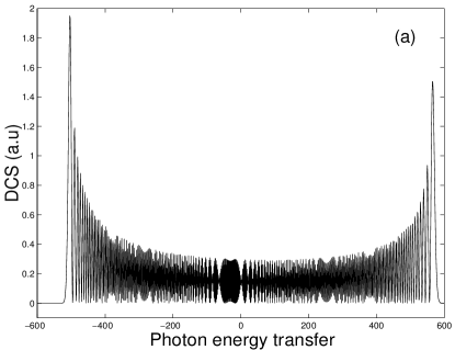
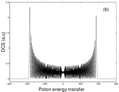
Figure 1: (a): Envelope of the non relativistic differential cross-section $d\sigma/d\Omega$ scaled in unit of $10^{-7}$ $a.u$ as a function of energy transfer $Q_{f}-Q_{i}$ scaled in units of the laser photon energy $w$ for an electric field strength of $0.05\,a.u$. and a relativistic parameter $\gamma=1.0053\,a.u$, (b). Envelope of the relativistic differential cross-section $(d\sigma/d\Omega)_{DV}$ scaled in unit of $10^{-7}$ $a.u$ as a function of the laser photon energy $w$ for the same parameters. The envelope for $(d\sigma/d\Omega)_{DV}^{\cite[cite]{[\@@bibref{}{1}{}{}]}}$ and $(d\sigma/d\Omega)_{KG}$ are almost identical

The observed cutoffs occur at $s_{min}=-522$ and $s_{max}=582$ for the non relativistic DCS and $s_{min}=-474$ and $s_{max}=474$ both for the Dirac-Volkov and Klein-Gordon DCSs since the argument that appears in the ordinary Bessel functions is the same for both DCSs. So the comments made in [1] concerning the interpretation of the envelope obtained do not apply for the Dirac-Volkov and Klein-Gordon cases. While the spectrum of Figure (1.a) of our work (which is identical to that of Figure (1.a) of [1]) exhibits an overall asymmetric envelope with peaks of negative energy transfer higher than peaks of positive energy transfer, this asymmetry is less pronounced in the case of the Dirac-Volkov and spinless particle DCSs. This emphasized asymmetry in the non relativistic case can easily be traced back by a close look at Eq.(34) of [1]. Indeed, the non relativistic DCS depends on $J_{s}^{2}(z)$ ($z$ depends only weakly on $s$) so the asymmetry can only come from the dependence of the modulus of the final momentum $\mathbf{q}_{f}$ on the number of the transferred photons $s$ according to Eq.(25) of [1]. We explicitly write this equation (with our notation)

$$|\mathbf{q}_{f}|=\left(|\mathbf{q}_{i}|^{2}+2s\frac{wQ_{i}}{c^{2}}+s^{2}\frac{w^{2}}{c^{2}}\right)^{1/2}.$$ (80)

Also, the denominator $|\mathbf{q}_{i}-\mathbf{q}_{f}+s\mathbf{k}|^{4}$ depends linearly on the number $s$ of transferred photons and this gives rise to an asymmetric envelope for the non relativistic DCS. In Figure 2, we plot the behaviour of $|\mathbf{q}_{i}-\mathbf{q}_{f}+s\mathbf{k}|^{-4}$ as a function of the number $s$ of photons transferred.

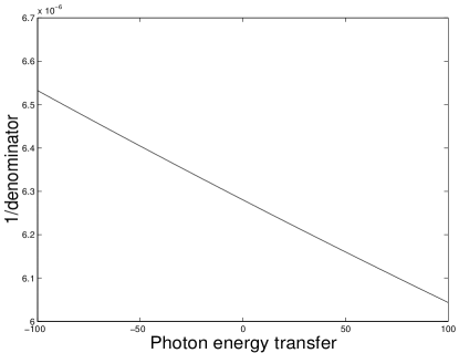
Figure 2: Behaviour of $|\mathbf{q}_{i}-\mathbf{q}_{f}+s\mathbf{k}|^{-4}$ as a function of the number $s$ of the photons transferred with $\gamma=1.0053$ and $\varepsilon=0.05\,a.u$

As mentioned in [1], we have an enhancement of negative over positive-energy transfer cross-section. The DCSs fall of abruptly beyond the points where the argument of the Bessel functions equal to the order. For the Dirac-Volkov and Klein-Gordon DCSs, this cutoff occurs ( up to machine precision) numerically for $s=\pm 474$ and an argument $z$ of the ordinary Bessel functions almost constant and equal to $380.016$. However Figure (1.b) shows a visual cutoff for $s=\pm 392$ since the infinitesimal contributions to the DCSs cannot be plotted. For the non relativistic DCS, the numerical cutoff occurs (again up to machine precision) for $s=-606$ and $s=685$. The visual cutoff occurs for $s=-500$ and $s=590$. The difference $\Delta s=20$ between our results and that of [1] is just a matter of convention. We now analyze the angular distributions. We have summed as in [1] $\pm 100$ peaks around the elastic one in order to draw the angular dependence of the DCS. In Figure 6. of [1], the accumulated DCS is shown for an electric field strength $\varepsilon=0.05\,a.u$. The computer code we have written calculates the Dirac-Volkov DCS (46) of our work, the Dirac-Volkov DCS (26) of [1], the spinless particle DCS and the non relativistic DCS. At least, in the non relativistic regime, our results and that of [1] agree very well and are both close to the results for a spinless particle. We give in Figure 3 the angular distribution of the various DCSs.

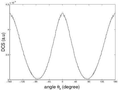
Figure 3: Summed differential cross sections $d\sigma/d\Omega$ of $\pm 100$ peaks around the elastic one as a function of the angle $\theta_{f}$ for a relativistic parameter $\gamma=1.0053\,a.u$ and an electric field strength $\varepsilon=0.05\,a.u$. The solid line denotes the result for Dirac-Volkov electrons, the long dashed one sketches the values for $(d\sigma/d\Omega)_{DV}^{[1]}$ and the short dashed is the result for spinless particles

Apart from minor differences, all three calculations exhibit maxima for $\theta_{f}=0^{\circ}$ and $\pm 180^{\circ}$, a giggling oscillatory behaviour (as in [1]) and minima slightly shifted from $\pm 90^{\circ}$ ( at $\pm 84^{\circ}$). Let aside the order of magnitude, we have in our case, three DCSs that are close to each other and not as differentiated as shown in Figure 6. of [1]. We do not agree at all with the results shown in Figure 6. In particular, our extrema for the various DCSs are shown in table (2) (scaled in $10^{-6}\,a.u$).

$\theta_{f}$	$(d\sigma/d\Omega)_{DV}$	$(d\sigma/d\Omega)_{DV}^{[1]}$	$(d\sigma/d\Omega)_{KG}$
$-180^{\circ}$	4.32027	4.32027	4.34311
-$84^{\circ}$	3.01486	3.01486	3.03079
$0^{\circ}$	4.326	4.326	4.34886
$84^{\circ}$	3.01486	3.01486	3.03079
$180^{\circ}$	4.32027	4.32027	4.34311

Table 2:

So, this adds to the controversy. Even if we use the expression for the Dirac-Volkov DCS given by Eq.(26) of [1], we have a different figure for the non relativistic regime. If we now increase the electric field strength from $\varepsilon=0.05\,a.u$ to $\varepsilon=1.00\,a.u$, the agreement remains good between the three relativistic calculations. There is still a maximum at $\theta_{f}=0^{\circ}$ while the minima are shifted towards $\pm 117^{\circ}$. To give an idea the small differences between our result and the result of [1] for the Dirac-Volkov DCS, we have plotted in the upper part (a) of Figure 4, the ratio of the DCS given by Eq.(26) of [1] to the DCS given by Eq.(46) of our work as a function of the angle $\theta_{f}$ for $\varepsilon=1.00\,u.a$. The ratio $R$ is defined by

$$R=\frac{(\frac{d\sigma}{d\Omega_{f}})_{DV}^{[1]}}{(\frac{d\sigma}{d\Omega_{f}})_{DV}}.$$ (81)

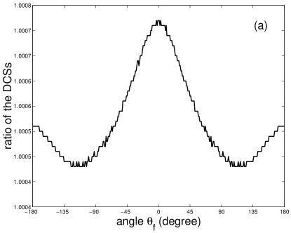
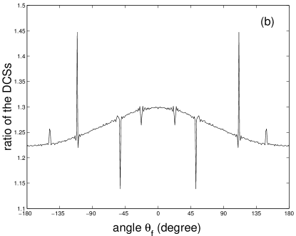
Figure 4: (a) Ratio $R$ of the two Dirac-Volkov DCS for $\gamma=1.0053,\,\varepsilon=1.00\,a.u$ and $s=\pm 100$. (b): Ratio $R$ of the two Dirac-Volkov DCS for $\gamma=1.0053\,a.u,\,\varepsilon=5.00\,a.u$ and $s=\pm 100$

The deviations from the expected value 1 are shown and have the same shape as the corresponding DCS. However, for increasing electric field strength, the values for this ratio are not close to 1. For a relativistic parameter $\gamma=1.0053\,a.u$ and for an electric field strength $\varepsilon=5.00\,u.a$ and $s=\pm 100$, our results for the Dirac-Volkov DCS and the corresponding results of [1] do not agree at all. In the lower part (b) of Figure (4), there is an over estimation varying from $22.5\%$ to $30\%$ with some peaks giving an over estimation of up to $45\%$ for the DCS (26) of [1] compared to the corresponding DCS (46) of this work. All these peaks are nearly multiples or submultiples of an angle close to $\pi/4$.

4.3 Relativistic-strong electric field strength regime

For the relativistic regime, we have chosen the parameters of [1] $\gamma=2$ which corresponds to an incoming electron total energy $E_{i}=2c^{2}$ or a $T_{i}=0.5116\,MeV$. The electric field strength is now $\varepsilon=1.00\,a.u$. Some cosines of the angles $\cos(\widehat{\mathbf{q}_{i},\mathbf{q}_{f}})$ and $\cos(\widehat{\mathbf{p}_{i},\mathbf{p}_{f}})$ are shown in Table (3)

$\cos(\widehat{\mathbf{p}_{i},\mathbf{p}_{f}})$	$\cos(\widehat{\mathbf{q}_{i},\mathbf{q}_{f}})$
0.853553	0.855757
0.850868	0.852775
0.847923	0.849543
0.844719	0.846062
0.841259	0.842332

Table 3:

In this regime, dressing effects are important. The envelope of the energy distribution of the scattered electrons is similar to the one displayed in the lower part (b) of Figure 1. However, there is a more important asymmetry than in the non relativistic regime with was to be expected. The corresponding cutoffs are $(-170000,194000)$ for ${(\frac{d\sigma}{d\Omega_{f}})}_{NR}$ and $(-66000,64000)$ for ${(\frac{d\sigma}{d\Omega_{f}})}_{DV}$,${(\frac{d\sigma}{d\Omega_{f}})}_{DV}^{[1]}$ and ${(\frac{d\sigma}{d\Omega_{f}})}_{KG}$. The three relativistic calculations lead to angular distributions peaked in the direction of the laser propagation $\theta_{f}=0^{\circ}$. The two Dirac-Volkov DCSs (solid line and long dashed line) are slightly different only in the vicinity of the two minima located at $\theta_{f}\simeq\pm 33^{\circ}$. In this regime, the shape of the ratio $R$ is similar to that of the corresponding DCSs. This ratio is equal to $1$ for $\theta_{f}=180^{\circ}$ but there is now an overall amplitude of $8.10^{-3}$ around the expected value $1$. If we increase the electric field strength from $\varepsilon=1.00\,a.u$ to $\varepsilon=5.89\,a.u$ and keep the same value of the relativistic parameter $\gamma=2$, the difference between our Dirac-Volkov results and the corresponding results of $[1]$ becomes important.
In the upper part(a) of Figure 5, we give the two Dirac-Volkov DCSs and in the lower part (b) of the same figure we give the ratio $R$ of the two DCSs for the relativistic parameter $\gamma=2.00$ and an electric field strength $\varepsilon=5.89\,a.u$. For the angles $\theta_{f}=\pm 180^{\circ}$, the ratio is $R\simeq 1.01$ while for the peak in the direction of the laser propagation, $\theta_{f}=0^{\circ}$, the ratio is $R\simeq 2.34$.

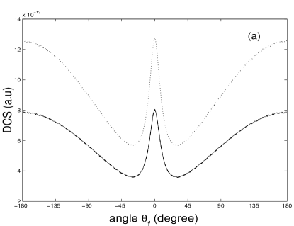
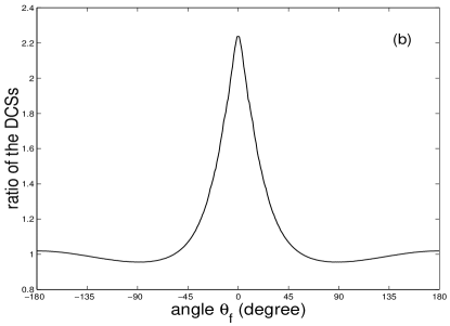
Figure 5: (a) Summed differential cross sections $d\sigma/d\Omega$ of $\pm 100$ peaks around the elastic one as a function of the angle $\theta_{f}$ for a relativistic parameter $\gamma=2.00$ and an electric field strength $\varepsilon=1.00\,a.u$. The solid line denotes the result for the Dirac-Volkov electrons, the long dashed one sketches the values for $(d\sigma/d\Omega)^{[1]}_{DV}$ and the short dashed is the result for spinless particles. (b): Ratio $R$ of the two Dirac-Volkov DCSs for a relativistic parameter $\gamma=2.00\,a.u$ and an electric field strength $\varepsilon=5.89\,a.u$

4.4 Relativistic and high electric field strength regime

To study this regime, we use the same parameters as in [1], that is a relativistic parameter $\gamma=5$ or an incoming electron kinetic energy $T_{i}=4c^{2}\,a.u=2.045\,Mev$. The electric field strength is $\varepsilon=5.89\,a.u$. In table(4), some cosines of the angles $cos(\widehat{\mathbf{q_{i},\mathbf{q_{f}}}})$ and $cos(\widehat{\mathbf{p_{i},\mathbf{p_{f}}}})$ are given. In this regime, the dressing of the electron angular coordinates is very important.

$\cos(\widehat{\mathbf{p}_{i},\mathbf{p}_{f}})$	$\cos(\widehat{\mathbf{q}_{i},\mathbf{q}_{f}})$
0.853553	0.866661
0.850868	0.861677
0.847923	0.856549
0.844719	0.851270
0.841259	0.845833

Table 4:

In the upper part (a) of Figure 6, we show the various DCSs.

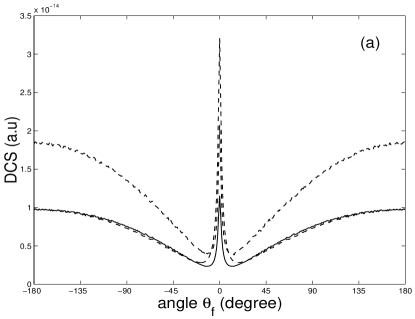
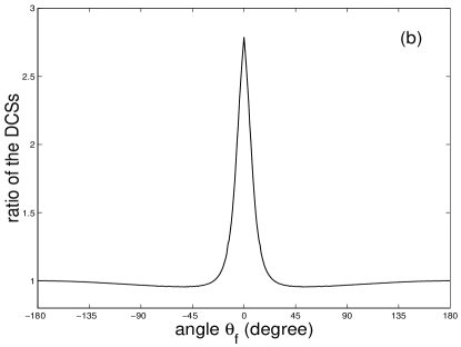
Figure 6: (a): Summed differential cross section $d\sigma/d\Omega$ of $\pm 100$ peaks around the elastic one as a function of the angle $\theta_{f}$ for a relativistic parameter $\gamma=5.00\,a.u$ and an elastic field strength $\mathbf{\varepsilon}=5.89\,a.u$. Th solid line denotes the result for Dirac-Volkov electrons, the long dashed one sketches the values for ${(d\sigma/d\Omega)_{DV}^{\cite[cite]{[\@@bibref{}{1}{}{}]}}}$ and the short dashed is the result for spinless particles. (b): Ratio $R$ of the two Dirac-Volkov DCSs for the same values of the relevant parameters, $\gamma=5.00\,a.u$ and $\mathbf{\varepsilon}=5.89\,a.u$

.

For angles $\theta_{f}=\pm 180^{\circ}$, the agreement between our results and the results of [1] is good but deteriorates for small values of $\theta_{f}$. For $\theta_{f}=0^{\circ}$, the result of our work gives a value ( scaled in $10^{-14}\,a.u$ ) $(\frac{d\sigma}{d\Omega_{f}})_{DV}=1.15$ while de corresponding result found using Eq.(26) of [1] is $(\frac{d\sigma}{d\Omega_{f}})_{DV}^{\cite[cite]{[\@@bibref{}{1}{}{}]}}=3.204$ . Our results (solid line) are always smaller than the results for spinless particles while those obtained using Eq.(26) of [1] are greater than $(\frac{d\sigma}{d\Omega_{f}})_{KG}$ for small angles around the direction of the laser propagation. In the lower part (b) of Figure 6, we show the ratio R defined by Eq.(81). For $\theta_{f}=0^{\circ}$, this ratio is $R=2.787$.

5 Conclusion

In this work, we derived the correct expression of the first Born differential cross section for the scattering of the Dirac-Volkov electron by a Coulomb potential of a nucleus in the presence of a strong laser field. We have given the correct relativistic generalization of the Bunkin and Fedorov treatment [7] that is valid for an arbitrary geometry. We are adamant that the core of the whole controversy stems from the fact that in [1], the vector $\eta^{\mu}$ introduced in Eq.(60) of our work has not been properly dealt with while it is the common method to use when a trace contains a $\gamma^{0}$ matrix. Any standard QED textbook introduces this very elementary method. Comparison of our numerical calculations [9] with those of Szymanowski et al. [1] shows qualitative and quantitative differences when the incoming total electron energy and the electric field strength are increased particularly in the direction of the laser propagation. The difference between our results and those of [1] can only be traced back to the mistakes and the omitted term in Eq.(26) of [1]. The corrections that we made allowed us to study other processes that were published in Physical Review A., namely an first article concerning the relativistic electronic dressing in laser assisted electron-hydrogen elastic collisions [10], another concerning the process of Mott scattering in an elliptically polarized laser field [11] as well as a third work dealing with the process of Mott scattering of polarized electrons in a strong laser field [12]. For the difficult process of ionization of atomic hydrogen by electron impact, we published an article concerning the importance of the relativistic electronic dressing in laser-assisted ionization of atomic hydrogen by electron impact [13]. All these works relied heavily on the corrections that we made in this work.

References

- [1] C. Zsymanowski, V. Véniard, R. Taïeb, A. Maquet and C.H. Keitel, Phys. Rev. A, 56, 3846, (1997).
- [2] V. G. Bagrov and D. M. Gitman, Exact solutions of relativistic Wave Equations (Kluwer Academic Publishers, Dordrecht, 1990)
- [3] D. M. Volkov, Z. Phys, 94, 250,(1935).
- [4] A. C. Hearn, Reduce User’s and Contributed Packages Manual, Version 3.7 (Konrad-Zuse-Zentrum f r Informationstechnik, Berlin, 1999).
- [5] V. Berestetzkii, E. M. Lifshitz and L. P. Pitaevskii, Quantum Electrodynamics, 2nd ed. (Pergamon Press, Oxford, 1982).
- [6] A. G. Grozin, Using Reduce in High Energy Physics (Cambridge University Press, 1997).
- [7] F.V. Bunkin and M.V. Fedorov, Zh Eksp. teor. Fiz. 49, 1215, (1965)[Sov. Phys. JETP 22, 844 (1966)].
- [8] Y. Attaourti, B. Manaut, e-print hep-ph/0207200.
- [9] Y. Attaourti, B. Manaut, Phys. Rev. A, 68, 067401, (2003).
- [10] Y. Attaourti, B. Manaut and A. Makoute, Phys. Rev. A, 69, 063407, (2004).
- [11] Y. Attaourti, B. Manaut and S. Taj, Phys. Rev. A, 70, 023404, (2004).
- [12] B. Manaut, S. Taj and Y. Attaourti, Phys. Rev. A, 71, 043401, (2005).
- [13] Y. Attaourti and S. Taj, Phys. Rev. A, 69, 063411, (2005).