One-Dimensional Motion of Bethe-Johnson Gas
Alex Granik
Department of Physics
University of thePacific
Stockton,CA.95211
E-mail: agranik@pacific.edu

ABSTRACT

A one dimensional motion of the Bethe-Johnson gas is studied in a context of Landau’s hydrodynamical model of a nucleus-nucleon collision. The expressions for the entropy change, representing a generalization of the previously known results, are found. It is shown that these expressions strongly depend on an equation of state for the baryonic matter.

1 INTRODUCTION

The application of special relativistic gasdynamics to some problems in particle physics goes back to the pioneering work by L.Landau [1] who obtained the asymptotic solution describing a one-dimensional expansion of a finite slab of matter modelled by the ultra-relativistic gas with the adiabatic index $\gamma=4/3$. Later I.Khalatnikov [2] obtained the exact solution of the same problem. G.Milekhin [3] extended this solution to an ultra-relativistic gas with an arbitrary adiabatic index. S.Belenkiy and G.Milekhin [4] applied a model of the ultra-relativistic shock wave to a problem of an entropy increase in a high energy nucleus-nucleon collision. A significant input into the problems associated with a hydrodynamical model of nucleus-nucleon collisions was made by G.Baym [5] who solved the Landau problem [1] for the cylindrical geometry. Nonetheless G.Baym and collaborators indicated that there is a need to use a more realistic equation of state than the one with $\Gamma=4/3$. Since there is still some uncertainty about an exact form of the equation of state for the baryonic matter at very high densities, one can consider a wide range of possible candidates for such an equation.

One of these equations was proposed by H.Bethe and M.Johnson [6] (which in what follows we call $BJ$ equation), and later it was used to illustrate an idea of a possible baryon-quark transition [7]. This equation was also used for a speculation on a potential influence of such a transition on a collective flow in a high energy ion collisions [8]. Therefore, it seems reasonable that a study of one-dimensional motions of Bethe-Johnson gas( including the original Landau problem) might provide a new insight into high energy phenomena within a model based on relativistic gasdynamics.

2 SHOCK ADIABATICS OF BJ GAS

We begin by considering a relativistic shock. In what follows we adopt the units with the speed of light taken to be $c=1.$ The energy, momentum, and particle conservation laws across the shock (in the shock frame)yield the following shock adiabatic [9]

$$\mu_{1}-\mu_{2}+\frac{1}{2}(p_{1}-p_{2})(\hat{V}_{1}+\hat{V}_{2})=0$$ (1)

where indices $1$ and $2$ denote the areas in front and the back of the shock respectively, $\mu\equiv W^{2}/2$, $W=w/n,~{}~{}~{}w=\epsilon+p$ is the enthalpy per unit of volume per unit of baryon rest mass, $n$ is the particle density, $p$ is the pressure per unit of baryon rest mass, $\epsilon$ is the energy density per unit of baryon rest mass,

$$\hat{V}=W/n=w/n^{2}$$ (2)

is the generalized ”specific volume” [10]. In these variables the relativistic shock adiabatic (1) looks exactly as the Hugoniot adiabatic of a newtonian gas.

2.1 SOME RELATIONS FOR A RELATIVISTIC SHOCK

We provide a series of relations which follow from the conservation laws across the shock. From the continuity of particle flux density

$$J\equiv n_{1}U_{1}=n_{2}U_{2}$$

and momentum flux density

$$(\frac{W}{n})_{1}U_{1}^{2}+p_{1}=(\frac{W}{n})_{2}U_{2}^{2}+p_{2}$$

(where we use the definition $W=w/n$) we obtain

$$J^{2}=\frac{p_{2}-p_{1}}{\hat{V}_{1}-\hat{V}_{2}}$$ (3)

indicating that either

$$a)p_{2}>p_{1},~{}~{}~{}\hat{V}_{1}>\hat{V}_{2}$$

$$b)p_{2}<p_{1},~{}~{}~{}\hat{V}_{1}<\hat{V}_{2}$$ (4)

in exact analogy to the newtonian case.It has turned out that only case $a)$ can actually occur.

This is easily shown by considering a relativistic weak shock wave, in which the discontinuity in every quantity is small as compared to the quantity. Let us expand both sides of the shock adiabatic (1) in powers of small differences of entropy(per unit of volume) $\Delta s\equiv s_{2}-s_{1}$ and pressure $\Delta p\equiv p_{2}-p_{1}$. Following the analogous procedure in newtonian gasdynamics, the expansion in $\Delta p$ is to be carried as far as the third order. Thus we obtain:

$$\mu_{1}-\mu_{2}=W_{1}^{2}-W_{2}^{2}=(\frac{\partial W^{2}}{\partial s})_{1}\Delta s+(\frac{\partial W^{2}}{\partial p})_{1}\Delta\ p+$$

$$(\frac{1}{2}\frac{\partial^{2}W^{2}}{\partial p^{2}})_{1}(\Delta p)^{2}+\frac{1}{6}(\frac{\partial^{3}W^{2}}{\partial p^{3}})_{1}(\Delta p)^{3}$$ (5)

where according to the thermodynamic identities,

$$(\frac{\partial W}{\partial s})_{p}=T~{}(the~{}absolute~{}~{}temperature),~{}~{}~{}~{}~{}~{}~{}~{}~{}~{}~{}~{}~{}~{}(\frac{\partial W}{\partial p})_{s}=V$$

Therefore (2.1) yields:

$$\ \mu_{1}-\mu_{2}=2W_{1}T_{1}\Delta s+2W_{1}V_{1}\Delta p+[V_{1}^{2}+W_{1}(\frac{\partial V}{\partial p_{1}})_{s}](\Delta p)^{2}+$$

$$[V_{1}(\frac{\partial V}{\partial p_{1}})_{s}+\frac{W_{1}}{3}(\frac{\partial^{2}V}{\partial p_{1}^{2}})_{s}](\Delta p)^{3}$$ (6)

The generalized ”specific volume” $\hat{V}=WV$ needs to be expanded only in terms of $\Delta p$, since the terms with $\Delta s$ contribute to the fourth order of smallness in $\Delta p$. Thus we get after some algebra:

$$\hat{V}_{2}-\hat{V}_{1}=W_{2}V_{2}-W_{1}V_{1}=[V_{1}^{2}+W_{1}(\frac{\partial V}{\partial p_{1}})_{s}](\Delta p)^{2}(\Delta p)+\frac{1}{2}[3V(\frac{\partial V}{\partial p_{1}})_{s}]\Delta p^{2}$$ (7)

where once again we use the thermodynamic identity $V=(\partial W/\partial p)_{s}$. Substituting this expansion together with (2.1) in (1). we obtain

$$\Delta s=s_{2}-s_{1}=\frac{1}{12T_{1}W_{1}}(\frac{\partial^{2}\hat{V}}{\partial p_{1}^{2}})_{s}(p_{2}-p_{1})^{3}$$ (8)

which once gain represents the exact analogy of the respective relation in newtonian gasdynamics (e.g., Ref. [1]). In all cases that have been studied the second derivative

$$(\frac{\partial^{2}\hat{V}}{\partial p_{1}^{2}})_{s}>0$$

Therefore by the law of increase of entropy $s_{2}>s_{1}$ and according to (8) $p_{2}>p_{1}$, which implies (Eq.2.1) $\hat{V}_{1}>\hat{V}_{2}.$

It was also shown [9] that a weak relativistic shock waves propagates with a speed of sound $c_{s}^{2}=(\partial p/\partial e)_{s}.$ In fact, for small $p_{2}-p_{1}$ and $\hat{V}_{2}-\hat{V}_{1}$ relation (3) can be written, in the first approximation, as

$$J^{2}=-(\frac{\partial p}{\partial\hat{V}})_{s}$$

In the same approximation

$$U_{1}^{2}=U_{2}^{2}=U^{2}=J^{2}V^{2}=-V^{2}(\frac{\partial p}{\partial\hat{V}})_{s}$$ (9)

On the other hand,

$$(\frac{\partial p}{\partial\hat{V}})_{s}=(\frac{\partial p}{\partial e})_{s}\frac{1}{[(\partial\hat{V}/\partial e)_{s}}$$

where by using the identity

$$-p(\frac{\partial V}{\partial e})_{s}=[\frac{\partial(eV)}{\partial e}]_{s}=e(\frac{\partial V}{\partial e})_{s}+V$$

we find

$$(\frac{\partial V}{\partial e})_{s}=-\frac{1}{n^{2}}(\frac{\partial n}{\partial e})_{s}=-\frac{V}{w}=-\frac{1}{nw}$$ (10)

and

$$(\partial\hat{V}/\partial e)_{s}\equiv(\frac{\partial wV^{2}}{\partial e})s\equiv V^{2}[\frac{\partial(e+p)}{\partial e}]_{s}+2Vw(\frac{\partial V}{\partial e})_{s}=$$

$$V^{2}(1+c_{s}^{2})-2V^{2}=-V^{2}(1-c_{s}^{2})$$

As a result Eq.(9) yields

$$U^{2}=-V^{2}(\frac{\partial p}{\partial\hat{V}})_{s}=\frac{c_{s}^{2}}{1-c_{s}^{2}}\equiv U_{s}^{2}$$

2.2 SHOCK WAVE IN BJ GAS

We consider a shock wave propagating in a specific gas with the following equation of state (Bethe-Johnson gas)

$$p=(\nu-1)(\epsilon-n)$$ (11)

where $\nu$ is an arbitrary constant playing the role of the adiabatic index. If the gas in front of the shock is cold, that is $p_{1}=0$ , equation (11) yields for that region:

$$\epsilon_{1}=n_{1}$$ (12)

which implies $\mu_{1}=1$ and hence $\hat{V}_{1}=V_{1}$, that is the conventional specific volume.

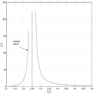
Figure 1: Pressure behind the shock $p_{2}$ as a function of $\hat{V}_{2}/V_{1}$ for $\nu=1.3$ and a cold gas ($p_{1}=0$) in front of the shock

By substituting Eqs.(11), (12) in the shock adiabatic (1) we obtain the following equation with respect to $p_{2}$

$$p_{2}[p_{2}V_{1}(\frac{\hat{V}_{2}}{V_{1}}\frac{1}{\nu-1}-1)^{2}-\frac{\hat{V}_{2}}{V_{1}}\frac{1}{\nu-1})(\nu+1)^{2}+1]=0$$ (13)

It has two solutions , one corresponding to a trivial case of a continuous flow with $p_{2}=p_{1}=0$ ( weak shock in this case), and the second one representing the strong shock wave:

$$p_{2}=(\nu-1)\frac{\hat{V}_{2}(\nu+1)-V_{1}(\nu-1)}{[\hat{V}_{2}-V_{1}(\nu-1)]^{2}}$$ (14)

A graph of $p_{2}V_{1}$ vs. $\hat{V}_{2}/V_{1}$ for a specific value of the ”adiabatic index” $\nu=1.3$ is shown in Fig.$1$.

From equation (14) follows that it has two branches ( as is clearly seen in the Fig.1), one for $\hat{V}_{2}/V_{1}\leq\nu-1$ and another one for $\hat{V}_{2}/V_{1}\geq\nu-1.$ We cannot determine the physical branch on the basis of the adiabatic only , since for both branches the conditions $p_{2}>p_{1},V_{2}<V_{1}$ [which follow from the law of entropy increase (8) and Eq.(11)] are satisfied in the region $(\nu-1)/(\nu+1)\leq\hat{V}_{2}/V_{1}\leq 1$. To choose the appropriate branch we find the adiabatic speed of sound in the region behind the shock, $(c_{s})_{2}$ ( it is obvious that in the region $1$ of the cold gas the speed of sound is $0$).

From (11) follows

$$(c_{s})_{2}^{2}=(\nu-1)[1-(\frac{\partial n_{2}}{\partial e})_{s}]=(\nu-1)(1-n_{2}V_{2})$$ (15)

where we use (10). We express this speed of sound in terms of $\hat{V}_{2}$. From (2) and

$$w=\frac{\nu}{\nu-1}p_{2}+\frac{1}{V}_{2}$$

[ which follows from (11)] we find

$$\hat{V}_{2}\equiv w_{2}V_{2}^{2}=\frac{\nu}{\nu-1}p_{2}V_{2}^{2}+V_{2}.$$

Solving this equation with respect to $V_{2}$ we obtain

$$V_{2}=(\nu-1)(\frac{\sqrt{1+4\frac{\nu}{\nu-1}p_{2}\hat{V}_{2}}-1}{2\nu p_{2}})$$ (16)

Therefore

$$w_{2}V_{2}=\frac{\hat{V}_{2}}{V_{2}}=\frac{2\nu}{\nu-1}\frac{p_{2}\hat{V}_{2}}{\sqrt{1+4\frac{\nu}{\nu-1}p_{2}\hat{V}_{2}-1}}$$

Inserting this in (15) and using (14) we get

$$(c_{s})_{2}^{2}=(\nu-1)\frac{(\nu-1)-\hat{V}_{2}/V_{1}}{\nu\hat{V}_{2}/V_{1}}$$ (17)

Now it becomes clear that for realistic values of $\nu\geq 1$

$$\frac{\hat{V}_{2}}{V_{1}}\leq(\nu-1)$$

(that is $(c_{s})_{2}^{2}\geq 0$) chooses the physical branch of the adiabatic (14), that is only the left part of the Fig.1 has a physical meaning.

We also demonstrate that the value of parameter $\nu$ cannot exceed $2$, since otherwise the flow becomes non-causal. Actually, from the boundaries

$$\frac{\nu-1}{\nu+1}\leq\frac{\hat{V}_{2}}{V_{1}}\leq(\nu-1)$$

(where the left inequality has been found above) of the physical region and relation (17) follows that the causality condition $(c_{s})_{2}^{2}\leq 1$ imposes the following restrictions on $\nu$

$$(\nu-1)^{2}\leq\frac{\nu-1}{\nu+1}(2\nu-1),~{}~{}~{}~{}~{}~{}~{}~{}that~{}is~{}1\leq\nu\leq 2$$ (18)

2.3 RATIO OF VELOCITIES BEHIND AND IN FRONT OF THE SHOCK

Here we derive equation for $\chi=\beta_{2}/\beta_{1}$ which is derived from the condition of continuity of the particle flux density

$$\frac{U_{2}}{U_{1}}=\frac{V_{2}}{V_{1}}.$$

Using (16) and the adiabatic (14) we obtain for its physical branch the following expression:

$$\frac{U_{2}}{U_{1}}=\frac{(\nu-1)-\frac{\hat{V}_{2}}{V_{1}}}{\nu}$$ (19)

We also provide the expression for $\chi=\beta_{2}/\beta_{1}$ found in [8],[11]:

$$U_{1}^{2}\chi^{2}-\nu U_{1}^{2}\chi+(\nu-1)(1+U_{1}^{2}-\sqrt{1+U_{1}^{2}(1-\chi^{2})}=0$$ (20)

Its implicit solution is:

$$\nu=1+U_{1}^{2}\chi\frac{\chi-1}{U_{1}^{2}(\chi-1)+\sqrt{1+U_{1}^{2}(1-\chi^{2}})}$$ (21)

The respective graph of $\chi=f(\nu,U_{1}^{2})$ is shown in Fig.2.

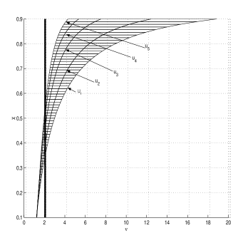
Figure 2: Ratio $\chi=\beta_{2}/\beta_{1}$ as a function of $\nu$ for $5$ values of the four-velocity $U_{1}$ from $.1$ to $3$

As is seen from the figure, for $5$ values of $\nu\leq 2$ ( which ensure the causality of the flow) parameter $\chi$ is always less than $\nu-1$.

For two asymptotic cases of

$i)$ a non-relativistic flow ($U_{1}\rightarrow\beta_{1}^{2}<<1$) and

$ii)$the ultra-relativistic flow ( with $U_{1}>>1$)

expression (21) is significantly simplified.

i)$U_{1}\rightarrow\beta_{1}<<1,\epsilon\rightarrow n,~{}~{}~{}\hat{V}_{2}\rightarrow V_{2}$. This allows us to rewrite (19) as follows

$$\frac{U_{2}}{U_{1}}=\chi[1-\frac{\beta_{1}^{2}}{2}(1-\chi^{2})]+O(\beta_{1}^{4})=\frac{\nu-1-\chi}{\nu}$$ (22)

By representing

$$\chi=\chi_{0}+\chi_{1}\beta_{1}^{2}$$

we obtain from (22) the final expression for $\chi$

$$\chi=\frac{\nu-1}{\nu+1}[1+\frac{2\nu^{2}}{(\nu+1)^{3}}\beta_{1}^{2}]+O(\beta_{1}^{4})$$ (23)

Using (23) and the fact that $\hat{V}_{2}/V_{1}\rightarrow V_{2}/V_{2}=\chi$ in the shock adiabatic (14) we obtain:

$$p_{2}V_{1}=\frac{2}{\nu+1}v_{1}^{2}$$

that is the result obtained in newtonian gasdynamics,(e.g., [1]). for a strong shock wave. This means that the lower part of the shock adiabatic ( close to $\hat{V}_{2}/V_{1}=(\nu-1)/(\nu+1)$, which seemingly contradicts the continuity of the particle density flux, actually represents the non-relativistic limit of the strong shock wave in Bethe-Johnson gas.

ii)$U_{1}>>1(\beta_{1}\rightarrow 1)$. Solving Eq.(20)we obtain

$$\chi\equiv\frac{\beta_{2}}{\beta_{1}}=(\nu-1)(1-\frac{1}{U_{1}}\sqrt{\frac{\nu}{2-\nu}})+O(1/U_{1}^{3})$$ (24)

which means that the velocity behind the shock

$$\beta_{2}\approx\nu-1$$

On the other hand,

$$\frac{U_{2}}{U_{1}}\equiv\frac{\chi}{\sqrt{1+U_{1}^{2}(1-\chi^{2})}}=\frac{1}{U_{1}}\frac{\chi}{\sqrt{1-\chi^{2}}}+O(1/U_{1}^{3})=\frac{(\nu-1)-\hat{V}_{2}/V_{1}}{\nu}$$ (25)

Using (24) in (25) we find with the same accuracy

$$\frac{\hat{V}_{2}}{V_{1}}=\chi=(\nu-1)(1-\frac{1}{U_{1}}\sqrt{\frac{\nu}{2-\nu}})+O(1/U_{1}^{2})$$ (26)

Upon substitution of (26) in shock adiabatic (14) we arrive at the following expression:

$$\frac{p_{2}}{n_{2}}\approx(1-\frac{\nu}{2})\frac{\nu-1}{1-\beta_{2}/(\nu-1)}\gg 1$$

$$and$$

$$\frac{p_{2}}{n_{1}}=\frac{p_{2}}{e_{1}}=(2-\nu)U_{1}^{2}\gg 1$$ (27)

It follows then that in this case

$$e_{2}\gg e_{1},$$

which in particular means that (2.3) is true even the particle number density is not conserved. The latter is easily verified by direct substitution of equations of state (11) and (12) in the laws of energy and momentum conservation.

It was suggested in [12] that for a compression ratio $n_{2}/n_{1}=5-20$ the baryon matter can be transformed into the quark gas. By using these values of $n_{2}/n_{1}$ in the shock adiabatic (14) we can find the range of the respective transition pressures $p_{2}$. By substituting

$$\frac{\hat{V}_{2}}{V_{1}}=\frac{\nu}{\nu-1}p_{2}\frac{n_{1}}{n_{2}^{2}}+\frac{n_{1}}{n_{2}},$$

which follows from the definition of $\hat{V}_{2}$ and the equation of state (11), we rewrite (14) as a function of $(n_{2}/n_{2},\nu):$

$$\nu^{2}z^{3}+z^{2}x[1-x(\nu-1)]+2(\nu-1)x^{2}\{[1-x(\nu-1)]^{2}-1-\nu^{2}\}$$

$$+x^{3}(\nu-1)^{3}[(\nu-1)x-\nu-1]=0$$ (28)

where $z=p_{2}n_{1}$ and $x=n_{2}/n_{1}$. If we fix the value of $e_{1}=n_{1}$ as $133MeV/fm^{3}$ ( based on the assumption that the ratio of the bag constant $B$ entering the bag model equation of state and $e_{1}$ is $0.45$ [10] and $B\approx 60Mev/fm^{3}$, then numerical solutions of (2.3)in terms of $p_{2}$ in $10^{35}dn/cm^{2}$ for the following values of the parameters

$$x=5,~{}8,~{}10;~{}~{}~{}~{}~{}~{}~{}~{}~{}\nu=1.7,~{}1.8,~{}1.9$$

are given in Table 1

Table I. Transition pressure $p_{2}$ for various values of $x=n_{2}/n_{1}$ and $\nu$

x =$n_{2}/n_{1}$	5	8	10
$\nu=1.7$	$3.51$	$42.37$	$37.88$
$\nu=1.8$	$5.68$	$27.31$	$49.30$
$\nu=1.9$	$10.67$	$34.76$	$42.66$

As is seen from the table, the transition pressure for $n_{2}/n_{1}=8$ and $10$ are of the same order of magnitude as the ones found in Ref. [13].

Now we consider the shock wave in an observer’s frame of reference such that the shock velocity is $-D$, the velocities in front and the back of the shock are $\beta_{1}$ and $\beta_{2}$ respectively. In the shock frame of references these velocities $\beta_{1,2}^{\prime}$ become

$$\beta_{1,2}^{\prime}=\frac{\beta_{1,2}+D}{1+\beta_{1.2}D}$$ (29)

From the conservation of energy and momentum across the shock follows that [9]

$$\beta_{1}^{\prime}\beta_{2}^{\prime}=\frac{p_{2}-p_{1}}{e_{2}-e_{1}}$$ (30)

Using equations of state for Bethe-Johnson gas (11) we obtain that for a strong shock ($U_{1}>>1$):

$$\beta_{2}^{\prime}\beta_{1}^{\prime}=(\nu-1)(1-\frac{1}{U_{1}}\sqrt{\frac{\nu}{2-\nu}})+O(U_{1}^{-2})\rightarrow\nu-1$$ (31)

Using (29) in (31) we get a quadratic equation with respect to $D$. The physical solution to this equation in terms of the velocities $\beta_{1},\beta_{2}$ in the observers frame of reference is

$$D=\frac{\sqrt{(2-\nu)^{2}(\beta_{1}+\beta_{2})^{2}+4[(\nu-1)-\beta_{2}\beta_{1}][1-\beta_{2}\beta_{1}(\nu-1)]}}{2[1-\beta_{1}\beta_{2}(\nu-1)]}$$

$$-\frac{(2-\nu)(\beta_{2}+\beta_{1})}{2[1-\beta_{1}\beta_{2}(\nu-1)]}$$ (32)

If $\nu\rightarrow 2$ then according to (2.3) $D\rightarrow 1.$ The respective graph of $D=f(\beta_{1},\beta_{2})$ for $\nu=1.3$ is shown in Fig. $3$.

Figure 3: Shock velocity $D$ in the observer frame as a function of the ratio of velocities $\beta_{1}$ and $\beta_{2}$ in front and behind the shock respectively

In what follows we need to have the ratio $W_{2}(\beta_{2})/W_{2}(0)$ where $W_{2}(\beta_{2})$ is the value of $W_{2}$ behind the shock (in the observer frame) and $W_{2}(0)$ is the respective value for $\beta_{2}=0$. Since in a strong shock $e>>n$,this implies

$$W_{2}\approx\frac{\nu}{\nu-1}p_{2}n_{2}$$

Therefore we get from (2.3)

$$\frac{W_{2}(\beta_{2})}{W_{2}(0)}=\frac{[1-\beta_{2}^{\prime}/(\nu-1)]_{\beta_{2}=0}}{[1-\beta_{2}^{\prime}/(\nu-1)]_{\beta_{2}}}$$ (33)

Since for a very strong shock wave $\beta_{1}\rightarrow 1$ the velocity $\beta_{1}^{\prime}$ also tends to $1$ according to (29). Therefore from (31) follows that $\beta_{2}^{\prime}\rightarrow\nu-1$. As a result, (33) becomes the indeterminacy of the type $0/0$. Using $l^{\prime}Hopitale$ rule we find (cf.[13])

$$[\frac{W_{2}(\beta_{2})}{W_{2}(0)}]_{\beta_{1}\rightarrow 1}=[\frac{(\partial\beta_{2}^{\prime}/\partial\beta_{1})_{\beta 2=0}}{(\partial\beta_{2}^{\prime}/\partial\beta_{1})_{\beta 2}}]_{\beta_{1}\rightarrow 1}$$ (34)

where

$$\partial\beta_{2}^{\prime}/\partial\beta_{1}=[\frac{\partial\beta_{2}^{\prime}}{\partial D}\frac{\partial D}{\partial\beta_{2}^{\prime}}]$$

Performing elementary calculations we find

$$[\frac{W_{2}(\beta_{2})}{W_{2}(0)}]_{\beta_{1}\rightarrow 1}=\frac{1-\beta_{2}}{1+\beta_{2}}$$ (35)

3 ONE-DIMENSIONAL SHOCK WAVE PROPAGATION

We consider the following problem [3]: $2$ shock waves propagate in opposite direction in a ”gas cylinder” as shown in Fig.$4$.

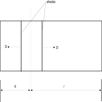
Figure 4: Geometry of $1$-dimensional shock waves propagation in the observer frame of reference

The distance travelled by the left-bound shock is denoted by $d$ and the respective distance travelled by the right-bound shock is denoted by $l$. A gas in front of both shocks is assumed to be ”cold”, that is its pressure is $p=0$. A compressed gas is taken to be Bethe-Johnson gas, obeying the equation of state (11). Initially we choose the frame of reference where the gas between $2$ shocks is at rest.

When the shock wave propagating to the left with a velocity $D$ reaches the left end of the cylinder, there begins an outflow of matter. As a result,a rarefaction wave has been formed which starts to move to the right with the speed of sound. At this time the shock wave moving to the right with a velocity $D$ has not yet reached the right end. Therefore the two possibilities can materialize:

a)the rarefaction wave can catch up and overtake the right-moving shock wave before it would reach the right end the right end of the cylinder,

or

b)the rarefaction wave will lag behind the right-moving shock wave.

If we use the shock frame of reference ( of the right-bound shock), then the gas velocity behind it is $D$, and in front of it is given by (29). We consider a strong shock, that is $\beta_{1}\rightarrow 1$ which implies that the respective velocity in the shock frame of reference is also $\beta_{1}^{\prime}\rightarrow 1$. Therefore combining the relation which is obtained by dividing energy and momentum fluxes across the shock ( see [13])

$$\beta_{1}^{\prime}=\frac{p_{2}+D^{2}e_{2}}{D(p_{2}+e_{2})}$$

and the equation of state (11) we obtain the quadratic equation for $D$ whose solution ( excluding the trivial root $D=1$) is

$$D=(\nu-1)\frac{p_{2}/n_{2}}{p_{2}/n_{2}+\nu-1}$$ (36)

Upon substitution of expression (2.3) for

$$p_{2}/n_{2}\rightarrow(1-\frac{\nu}{2})\frac{\nu-1}{1-\beta_{2}/(\nu-1)}\gg 1$$

( valid for a very strong shock with $\beta_{1}\rightarrow 1$ and $\beta_{2}\rightarrow\nu-1$) in (35) we obtain that

$$D\rightarrow\nu-1$$

This means that we can find the minimum length $l_{min}$ of the ”tunnel” such that the rarefaction wave overtakes the shock wave [13]

$$\frac{l_{min}+d}{(\beta_{s})_{2}}=\frac{l_{min}-d}{D}$$ (37)

where the speed of sound in gas behind the shock $(\beta_{s})_{2}$ is given by the following expression [9]

$$(\beta_{s})_{2}^{2}=(\nu-1)\frac{\nu p_{2}/n_{2}}{(\nu-1)+\nu p_{2}/n_{2}}$$ (38)

Taking into account that $p_{2}/n_{2}\gg 1$, we see that $(\beta_{s})_{2}\rightarrow\sqrt{\nu-1}$. Therefore from equation (37) we get

$$\frac{l_{min}}{d}=\frac{\sqrt{\nu-1}+1}{1-\sqrt{\nu-1}}$$ (39)

For the values of $\nu=1.3-1.9$ the respective $l_{min}/d$ varies from $3.42$ to $37.97$. In general $l_{min}/di$ is a monotonically increasing function which tends to infinity when $\nu\rightarrow 2$. As was shown in Refs.[3] and [13] the entropy change in the case of $l\leq l_{min}$ is

$$\Delta s\sim\frac{l}{d}+1$$

The problem becomes more involved if $l/d\geq l_{min}$, because the rarefaction wave can overtake the shock wave but cannot pass through it. Therefore the former is reflected from the latter thus creating the flow region bounded on one side by the shock wave moving to the right and on the other side by the reflected wave moving to the left. The resulting flow can be described with the help of the equation for a general one-dimensional motion of a relativistic gas [1]

$$\beta_{s}^{2}\frac{\partial^{2}\chi}{\partial y^{2}}+(1-\beta_{s}^{2})\frac{\partial\chi}{\partial y}-\frac{\partial^{2}\chi}{\partial\eta^{2}}=0$$ (40)

where

$$y=Ln(W/W_{0}),$$

$W_{0}$ is the value of $W$ behind the shock when the velocity $\beta_{2}=0$,

$$\eta=tanh^{-1}\beta$$ (41)

and the generalized potential $\chi$ is connected to the spatial $x$ and temporal $t$ coordinates as follows

$$x=e^{-y}(\frac{\partial\chi}{\partial y}sinh\eta-\frac{\partial\chi}{\partial\eta}cosh\eta)$$

$$t=e^{-y}(\frac{\partial\chi}{\partial y}cosh\eta-\frac{\partial\chi}{\partial\eta}sinh\eta)$$ (42)

By using (38) in (40) we obtain

$$(\nu-1)(1-\frac{e^{-y}}{W_{0}})\frac{\partial^{2}\chi}{\partial y^{2}}+(2-\nu+\frac{\nu-1}{W_{0}}e^{-y})\frac{\partial\chi}{\partial y}-\frac{\partial^{2}\chi}{\partial\eta^{2}}$$ (43)

For a strong shock wave $\beta_{s}^{2}\rightarrow\nu-1$, $W_{0}\gg 1,y>>1$, and equation (43) becomes

$$(\nu-1)\frac{\partial^{2}\chi}{\partial y^{2}}+(2-\nu)\frac{\partial\chi}{\partial y}-\frac{\partial^{2}\chi}{\partial\eta^{2}}=0$$ (44)

The respective boundary conditions are based on the fact that in the strong shock wave ( in the shock frame of reference) the velocity of gas behind the shock is $\beta_{2}^{\prime}=\nu-1$ (cf.[13]). Therefore from equation (29) follows that the shock velocity $D$ in terms of $\beta_{2}^{\prime}$ ( in the shock frame) and $\beta_{2}=-tanh\eta$ (in the observer frame) is

$$D=\frac{dx}{dt}=\frac{\nu-1+tanh\eta}{1+(\nu-1)tanh\eta}$$ (45)

On the other hand, from (35) and (41) follows that at the shock

$$y=2\eta$$ (46)

Because equation (2.3) is true for very strong shock waves, even if the particle number is not conserved, relation (46) remains valid in this case. If we use as model an ultra-relativistic gas then equation (2.3) is exact, although it refers to $e_{2}$ instead of $W_{2}$. In addition, the variable $y$ becomes [2]

$$y=Ln(\frac{T}{T_{0}})$$

where $T$ is the absolute temperature of the gas. Equation (46) is replaced in this case by the following

$$y=2\frac{\nu-1}{\nu}\eta$$ (47)

where $\nu$ is the arbitrary adiabatic index.

If in our problem (considering Bethe-Johnson gas) we assume that the particle numbers are not conserved then for a very strong compressive shock ( $W\sim p/n>>1$) thermodynamic calculations show that now

$$y\approx Ln(\frac{T}{T_{0}})$$

and

$$\frac{\sigma}{\sigma_{0}}\approx(\frac{T}{T_{0}})^{1/(\nu-1)}$$ (48)

where $\sigma$ is the entropy per unit of volume and we use $p\sim n^{\nu}$ We can combine both expressions (46) and (47) for $y$ into one generalized relation

$$y=\delta\eta$$ (49)

where $\delta$ can be either greater or less than $1$.

We substitute (49) in (45), use (3) and equation (44) and obtain ( after rather lengthy calculations) that at the shock ( where $y=\delta\eta$)

$$\{[(\delta+1)\frac{\partial}{\partial y}+(\frac{\delta}{\nu-1}+1)\frac{\partial}{\partial\eta}](1-\frac{\partial}{\partial y})\chi\}_{y=\delta\eta}=0$$ (50)

The other boundary condition (at the Riemann wave) is borrowed from Ref.[2]

$$\chi|_{\eta=y/\sqrt{\nu-1}}=0$$ (51)

By introducing new variables

$$q=\eta-\frac{y}{\delta},~{}~{}~{}~{}~{}~{}~{}~{}~{}~{}~{}~{}~{}~{}~{}~{}~{}h=\frac{y}{\sqrt{(\nu-1)}}-\eta$$

we rewrite equation (44)and the boundary conditions (50),(51)

$$[(\frac{\nu-1}{\delta^{2}}-1)\frac{\partial^{2}}{\partial q^{2}}+2(1-\frac{\sqrt{\nu-1}}{\delta})\frac{\partial^{2}}{\partial q\partial h}+\frac{2-\nu}{\sqrt{\nu-1}}\frac{\partial}{\partial h}-\frac{2-\nu}{\delta}\frac{\partial}{\partial q}]\chi=0$$ (52)

$$\{[(\frac{\delta+1}{\sqrt{\nu-1}}-\frac{\delta+\nu-1}{\nu-1})\frac{\partial}{\partial h}+\frac{\delta^{2}-nu+1}{\delta(\nu-1)}\frac{\partial}{\partial q}](1+\frac{1}{\delta}\frac{\partial}{\partial q}-\frac{1}{\sqrt{\nu-1}}\frac{\partial}{\partial h}\}\chi|_{q=0}=0$$ (53)

Applying Laplace transform to variable $h$ in equations (51)-(53) we obtain

$$(\frac{\nu-1}{\\ delta^{2}}-1)\frac{d^{2}\chi}{dq^{2}}+[2(1-\frac{\sqrt{\nu-1}}{\delta})r-\frac{2-\nu}{\delta}]\frac{d\chi}{dq}+\frac{2-\nu}{\sqrt{\nu-1}}r\chi=0$$ (54)

and

$$[(\frac{\delta+1}{\sqrt{\nu-1}}-\frac{\delta+\nu-1}{\nu-1})r+\frac{\delta^{2}-nu+1}{\delta(\nu-1)}\frac{d}{dq}](1+\frac{1}{\delta}\frac{d}{dq}-\frac{1}{\sqrt{\nu-1}}r)\chi|_{q=0}=0$$ (55)

where $r$ is the transformation parameter.

We represent a solution to (54), (55) as $a(r)e^{qk(r)}$. This leads to $2$ algebraic equations:

$$(1-\hat{\delta}^{2})\hat{k}^{2}+\hat{k}[2(\hat{\delta}-1)\hat{r}-\frac{2-\nu}{\nu-1}]+\frac{2-\nu}{\nu-1}\hat{r}=0$$ (56)

$$(\hat{k}+\frac{\sqrt{\nu-1}-1}{\hat{\delta}+1}\hat{r})(1+\hat{k}+\hat{r})a+\frac{1}{\sqrt{\nu-1}}\frac{\sqrt{\nu-1}-1}{\hat{\delta}+1}\hat{\lambda}=0$$ (57)

where

$$\hat{k}=\frac{k}{\delta},~{}~{}~{}~{}\hat{r}=\frac{r}{\sqrt{\nu-1}},~{}~{}~{}~{}~{}\hat{\delta}=\frac{\delta}{\sqrt{\nu-1}},~{}~{}~{}~{}~{}~{}\hat{\lambda}=\frac{\lambda}{\sqrt{\nu-1}}$$

In turn, the variable $\lambda$ is calculated at the point where Riemann’s wave catches up with the shock wave [4]

$$\lambda=(\frac{\partial\chi}{\partial q})|_{q=0,h=0}=-(\frac{\partial\chi}{\partial h})|_{q=0,h=0}$$

We will be interested in finding the entropy change in this flow. It is given by the following expression [4]

$$\Delta S=\Sigma_{0}\int_{t1}^{t_{2}}\sigma u_{2}dt$$ (58)

Here $\Sigma_{0}$ is the ”tunnel’s” cross-sectional area, $\sigma$ is the entropy density behind the shock, $u_{2}=\beta_{2}/\sqrt{1-\beta_{2}^{2}}$. $t_{1}$ is the moment of time when Riemann’s wave catches up with the shock wave and $t_{2}$ is the moment of time when the shock wave reaches the right end of the ”tunnel” (Fig.5). Since n we consider a strong shock $\beta_{2}\rightarrow\nu-1$, that is $u_{2}\approx(\nu-1)/\sqrt{2-\nu}$. Because the time interval $dt$ is measured in the shock frame reference the respective time interval in the observer frame ( where initially both waves, the strong shock and Riemann’s wave move with a velocity $D$) is $dt/\sqrt{1-D^{2}}$. Taking these facts into account and using (43),(45),(49) and (48) we obtain from (58)

$$\Delta S=\frac{\delta^{2}-\nu+1}{\delta(\delta+1)}\int_{0}^{y_{c}}e^{y(2-\nu)/(\nu-1)}[\frac{\partial}{\partial\eta}(\frac{\partial}{\partial y}-1)\chi]|_{y=\delta\eta}$$ (59)

where $y_{c}$ is the value of $y$ at the moment when the shock wave reaches the right end of the ”tunnel”.

By introducing variables $q$ and $h$ into (59) and effecting the integration we find after rather involved calculations

$$\Delta S=a_{1}([1-h^{\prime}e^{a_{2}}\pm a_{3}e^{h^{\prime}A}\int_{0}^{h^{\prime}_{c}}\frac{e^{-Az}-e^{-zF_{\pm}}}{h_{c}^{\prime}-z}Z_{\pm}(h_{c}^{\prime}-z)dz]$$ (60)

where

$$a_{1}=\frac{\pm\Sigma_{0}\sigma_{0}\lambda}{2}\frac{(A+\sqrt{A^{2}\mp 1})(1+\sqrt{\nu-1})}{A+\sqrt{A^{2}\mp 1}+A\sqrt{\nu-1}},$$

$$a_{2}=-2A\frac{\nu-1}{2-\nu}(1+\sqrt{\frac{1\mp A^{-2}}{\nu-1}}),$$

$$a_{3}=\frac{(A-\sqrt{A^{2}\mp 1})(\nu-2\sqrt{\nu-1}}{2-\nu},$$

$$A^{2}=\left\{\begin{array}[]{cc}\hat{\delta}^{2}/(1-\hat{\delta}^{2})&\mbox{for $\hat{\delta}<1$}\\ \hat{\delta}^{2}/(\hat{\delta}^{2}-1)&\mbox{for $\hat{\delta}>1,$}\end{array}\right.$$

$$h^{\prime}=\frac{h}{2\sqrt{\nu-1}}\frac{2-\nu}{A-\sqrt{A^{2}\mp 1}},$$

$$F_{\pm}=\frac{\nu A+2\sqrt{(A^{2}\mp 1)(\nu-1)}}{2-\nu},$$

$$Z_{\pm}=\left\{\begin{array}[]{ll}I_{1}(h_{c}^{\prime}-z)&\mbox{Bessel function of the imaginary argument}\\ J_{a}(h_{c}^{\prime}-z)&\mbox{Bessel function of the first kind},\end{array}\right.$$

and everywhere the upper and lower signs correspond to $A>1$ and $A<1$ respectively.

We also have to find the value of $h_{c}$ entering integral in (60). To this end we use the relation from Ref.[3]

$$x_{c}-l=t_{0}-t_{c}$$ (61)

where $t_{0}=\lambda/\sqrt{\nu-1}$ is the moment of time when Riemann’s wave overtake the shock wave ( in the observer’s frame), L is the coordinate corresponding to this location of the wave, $x_{c}$ and $t_{c}$ are the coordinate and moment of time describing the state of the shock weave at the right end of the ”tunnel”. Inserting $x$ and $t$ from (3) in (61) and performing rather lengthy calculations, we obtain

$$\frac{(L\sqrt{\nu-1}+\lambda)(\sqrt{\nu-1}-\nu+1)}{\lambda\sqrt{\nu-1}}=$$

$$\frac{2\sqrt{\nu-1}+\nu}{2A}\{A+\sqrt{A^{2}\mp 1}exp[-2\nu Ah^{\prime}/(2-\nu)]+A-\sqrt{A^{2}\mp 1}\}-$$

$$\frac{2-\nu}{2A}e^{-g_{\pm}h^{\prime}}\int_{0}^{h_{c}^{\prime}}\frac{e^{g_{\pm}z}-e^{f_{\pm}z}}{h_{c}^{\prime}-z}Z_{\pm}(h_{c}^{\prime}-z)dz$$ (62)

where

$$g_{\pm}=\frac{\nu A-2\sqrt{(A^{2}\mp 1)(\nu-1)}}{2-\nu},$$

$$f_{\pm}=-[\nu A+2\sqrt{(A^{2}\mp 1)(\nu-1)}]$$

In what follows we neglect the integral in (3) which would introduce an error not exceeding $2\%$.

From the kinematic considerations follow that

$$L+\frac{\lambda}{\sqrt{\nu-1}}=(l+d)+\frac{l-d}{\nu-1}$$

and

$$\lambda=d(\frac{D+\beta_{s}}{D-\beta_{s}}+1)$$

Therefore relation (3) (with the integral dropped) would yield the expression for $exp(-2Ah^{\prime}/\nu)$ in terms of $\nu$ and $A$

$$\pm(A+\sqrt{A^{2}\mp 1})^{2}exp(-\frac{2A\nu h^{\prime}}{2-\nu})=$$

$$\frac{1}{\sqrt{\nu-1}(A-\sqrt{A^{2}\mp 1})}[\nu A(1-\sqrt{\nu-1})\frac{l}{d}+\sqrt{(A^{2}\mp 1)(\nu-1)}-A(\nu-\sqrt{\nu-1})]$$ (63)

$i$) If $\delta=2(\nu-1)/\nu$ ( as in the case of an ultra-relativistic gas with an arbitrary constant adiabatic index $\nu$) implying $A=2\sqrt{\nu-1}/(2-\nu)$ then we choose in (60) the lower sign. As a result, we obtain from ( 60) with the help of (3)

$$\frac{\Delta S}{\Sigma_{0}\lambda\sigma_{0}}=\frac{3\nu-2+(\nu+2)\sqrt{\nu-1}}{2(3\nu-2)}\{[(\frac{2-\nu}{\nu+2\sqrt{\nu-1}})^{2}(\frac{2\nu}{2-\nu}\frac{l}{d}-1)]^{(3\nu-2)/2\nu}-1\}$$

where

$$\frac{l}{d}\geq\frac{1+\sqrt{\nu-1}}{1-\sqrt{\nu-1}}$$

The respective graph of $<\Delta S>\equiv\Delta S/(\Sigma_{0}\lambda\sigma_{0})$ is shown in Fig.5.

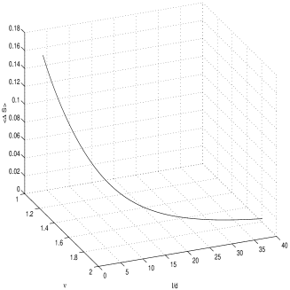
Figure 5: Variation of the dimensionless entropy change as a function of the adiabatic index $\nu$ and $l/d$

Expression given by (3) yields as a particular case the expression found in [4] for $\nu=4/3$ It is seen that the entropy change in region $2$ increases and reaches its maximum for the values of $\nu$ in the range from $1.3$ to $1.4$. A further increase of $\nu$ results in a sharp decline of the entropy change, approaching the purely adiabatic regime for the threshold value of $\nu=2$.
$ii)$ If, we consider $\delta=2$ ( as in 46) we obtain in the same fashion as in $i$:

$$\frac{\Delta S}{\Sigma_{0}\lambda\sigma_{0}}=\frac{3\sqrt{\nu-1}+\nu+1}{6\sqrt{\nu-1}}\{1-[1+\frac{2\nu}{\nu-1+2\sqrt{\nu-1}}(\frac{l/d}{l_{c}/d}-1)]^{3(\nu-1)/2\nu}\}$$ (65)

where $l_{m}/d$ is given by (39). From (65) follows that in this case the entropy change can be positive only if $\nu>2.$ However this also means that the flow becomes non-causal , since ( as we showed above) in this case $\beta_{s}>1.$ Therefore if $\delta=2$ the one-dimensional flow of Bethe-Johnson gas with $\nu<2$ is characterized by a zero change of entropy when Riemann’s wave catches up with the shock wave (and stays zero from that moment on), that is the flow becomes adiabatic. This contrasts with the previous case $i)$ which is a generalization of the analogous flow for an ultra-relativistic with an arbitrary adiabatic index ( not necessarily $\nu=4/3$ as in [4]). In the latter the entropy change is linear in $l/d$ before Riemann wave catches up with the shock wave, and obeys the power law for $l/d$ (given by eq.65) after Riemann wave overtakes the shock wave.

The flow described here can be associated with a nucleon-nucleon collision (cf.[13]) which is modelled as a collision of the nucleon with a cylinder cut out of the nucleus and whose cross-sectional area is equal to the one of the nucleus. The nucleus linear size varies from the diameter of the nucleus to the ”diameter” of the nucleon, $d$. It is clear that such an approximation can be used only to obtain certain estimates about parameters of the real process, for example to evaluate an entropy change. The ratio $l/d$ is related to the atomic number $\bf{A}$: $l/d={\bf{A}}^{1/3}.$ If we take $max{\bf{A}}=257$ this would give us the maximum value of $\nu=1.53$ ( according to eq.39)which is close to the region where entropy change reaches its maximum.

4 CONCLUSION

We found the shock adiabatic for BJ gas and applied the found detailed relations for a study of a one-dimensional flow of such a gas in a context of a nucleon-nucleon collision. If baryon matter can be transformed into quark matter at a certain range of the compression ratio ($5-10$), then the proposed model allows one to identify the baryon matter as Bethe-Johnson gas with the adiabatic index $\nu\approx 1.5.$

Such an approach generalizes an analogous approach based upon an ultra-relativistic gas. The latter represents a particular case of BJ gas with adiabatic index $\nu=4/3$. The entropy change behind the shock strongly depends on the choice of the adiabatic index in BJ, by reaching its maximum in the range of values of $\nu$ from $1.3$ to $1.4$.

References

- [1] L.Landau, 1953, Izv.Aca.Sci.USSR,Physics,17,51
- [2] I.Khalatnikov 1954, ZhETP, 27,529
- [3] G.Milekhin 1961, Trudy FIAN, 16,51
- [4] S.Belenkiy,G.Milekhin 1959, ZhETP, 29, 20
- [5] G.Baym,B.Friman et al. 1983, Nucl. Phys. A, 407,541; G.Baym, B. Friman and J.-P. Blaizot 1983, Phys. Lett.B 132,291 . G.Baym, B.Friman, et al. 1984 , Lecture Notes - Physics 198, Recent Progress in Many-Body Theories,Springer, New York,6.
- [6] H.Bethe and M.Johnson 1974, Nucl.Phys.A, 230,1
- [7] G.Chapline and M.Nauenberg 1977, Ann.N.Y.Aca.Sci.,302,191
- [8] G.Chapline and A.Granik 1986, Nucl.Phys.,459,681
- [9] A.Taub 1948, Phys.Rev.,74,328; L.Landau and E.Lifshitz 1959, Fluid Mechanics,Addison-Wesley Publ.Co.,Reading
- [10] K.Thorne 1973, ApJ,179,897
- [11] G.Chapline and M.Nauenberg 1977, Phys.Rev.D, 16,450
- [12] G.Chapline and M.Nauenberg 1977,Ann.N.Y.Aca.Sci.,302,191
- [13] S.Belenkiy and L.Landau 1956, Nuovo Cimento,Suppl.,3.15