Electronic Structure of Atoms in Magnetic Quadrupole Traps

Abstract

We investigate the electronic structure and properties of atoms exposed to a magnetic quadrupole field. The spin-spatial as well as generalized time reversal symmetries are established and shown to lead to a two-fold degeneracy of the electronic states in the presence of the field. Low-lying as well as highly excited Rydberg states are computed and analyzed for a broad regime of field gradients. The delicate interplay between the Coulomb and various magnetic interactions leads to complex patterns of the spatial spin polarization of individual excited states. Electromagnetic transitions in the quadrupole field are studied in detail thereby providing the selection rules and in particular the transition wavelengths and corresponding dipole strengths. The peculiar property that the quadrupole magnetic field induces permanent electric dipole moments of the atoms is derived and discussed.

I Introduction

External fields represent an excellent tool to influence and control the motion of quantum systems and in particular to generate new, sometimes very surprising, properties of e.g. atoms and molecules. In the case of static homogeneous magnetic fields the interest in the electronic structure of the hydrogen atom reached its maximum in the late 1980’s Friedrich89 . This was motivated on the one hand by the experimental accessibility of highly excited Rydberg states via laser spectroscopy as well as the astronomical observation of spectra from magnetic white dwarfs possessing a hydrogen-rich atmosphere Ruder94 . On the other hand the development of new numerical techniques allowed to address the regime where the competition of the Coulomb and diamagnetic interaction leads to unusual and complex properties and phenomena. Besides the vivid interest in magnetized structures the hydrogen atom served as a paradigm of a nonseparable and nonintegrable system possessing major impact with respect to the development of several fields such as quantum chaos, semiclassics of nonintegrable systems and nonlinear dynamics in general (see Friedrich89 ; Friedrich97 ; Schmelcher98 ; Schmelcher97 and references therein).

In contrast to the case of a homogeneous magnetic field there exist no investigations on the electronic structure and properties of atoms in inhomogeneous or trapping magnetic field configurations. Apart from the fact that this problem is of fundamental interest, experimental techniques allow nowadays to manufacture magnetic microtraps on atom chips Folman02 . The latter consists of surface-mounted structures carrying microscopic charges and/or currents which create a miniature landscape of inhomogeneous electric and/or magnetic fields. In particular it is possible to build tight magnetic traps which involve magnetic field configurations with large field gradients up to ${\mathcal{B}}\approx 10^{8}\frac{G}{cm}$. Since these traps strongly confine the atoms it is to be expected that the electronic structure of excited or highly excited Rydberg states is influenced significantly by the spatially varying field. Quadrupole magnetic fields represent a key configuration which is used in many setups of traps. We therefore investigate here the electronic structure of atoms exposed to a quadrupole magnetic field (see also ref.Lesanovsky04 ).

In detail we proceed as follows. In section II we present the electronic Hamiltonian of the atom in the quadrupole field including the interaction of the spatial as well as spin degrees of freedom with the external field. Section III contains a discussion of the remarkable spin-spatial symmetries of the Hamiltonian including unitary as well as antiunitary symmetries and the related constants of motion. As a result we encounter a two-fold degeneracy of each eigenstate. Section IV discusses the eigenstates obeying different symmetries and the resulting consequences for expectation values of observables. Section V briefly outlines our computational approach. In section VI we present the results of our numerical investigations establishing new spectral and other properties for low-lying and highly excited states for weak and strong gradients. The spin expectation values and in particular the spatial distribution of the spin polarization of the excited states are studied in detail. Electromagnetic transitions in the quadrupole field including dipole strengths and wavelengths are given too. Whereever appropriate a comparison with the case of a homogeneous magnetic field is performed. Finally the peculiar property of magnetic field-induced permanent electric dipole moments is derived and investigated in depth. Section VII contains the conclusions and outlook as well as some discussion of relevant aspects going beyond the present investigation.

II The Hamiltonian

In ultracold atomic physics moving atoms in inhomogeneous magnetic fields are considered to be neutral point-like particles which couple only through their total angular momentum to the external field Folman02 ; Bergeman89 . In slowly varying magnetic fields it is appropriate and convenient to describe the dynamics of the atoms by means of an adiabatic approximation, where one assumes that the magnetic moment is oriented either parallel or antiparallel to the magnetic field. In this way the interaction potential becomes proportional to the modulus of the magnetic field. As long as the spatial extent of the atom is much less than the typical variations of the field and if one is only interested in the center of mass motion of the atom the adiabatic approximation can be applied reliably.

In the present investigation we are interested in the electronic structure of excited atoms exposed to a quadrupole magnetic trap or field. Therefore we have to go beyond the above approximation in the sense that the detailed coupling of both the electronic spatial as well as the spin degrees of freedom to the external field is taken into account. The majority of todays experiments on ultracold atoms deal with alkali-atoms Folman02 . Alkali-atoms become rapidly hydrogen-like if their single valence electron is excited. The detailed structure of the core becomes increasingly irrelevant with increasing degree of excitation. We therefore assume that the outer electron is exposed to the field of a single positive point charge. Furthermore we neglect the spin-orbit ($LS$) coupling and the coupling of the nuclear and electronic spin, i.e. the hyperfine interaction. These interactions show an $r^{-3}$-dependence, i.e. a rapid decay with increasing $r$. Thus for sufficient highly excited states their contributions are negligible compared to those of the Coulomb-potential and the interaction with the external field. Nevertheless one can discuss how the inclusion of spin-orbit coupling might modify the properties of the system. For hydrogen in a homogeneous field this relativistic effect changes the symmetries of the system crucially: $S_{z}$ and $L_{z}$ are no longer conserved separately and only $J_{z}$ remains a conserved quantity. The result is a restructuring of the energy spectrum since previously separated symmetry sub-spaces become coupled. In particular this manifests itself in the emergence of avoided crossing Ruder94 . For the atom in the quadrupole field such dramatic effects are not expected since the additional $LS$-coupling term does not reduce the symmetry of the system. Additionally, considering its $r^{-3}$-dependence, the spin-orbit interaction can certainly be treated by means of perturbation theory in the regime of spatially extensive and energetically highly excited Rydberg states.

In the presence of a magnetic field the motion of the center of mass (CM) and internal (electronic) degrees of freedom of an atom do not decouple. This holds in particular for the case of a homogeneous magnetic field Lamb59 ; Avron78 ; Johnson83 ; Schmelcher94 and therefore has also to be expected for an inhomogeneous field. However, CM-motional effects on the electronic structure become only significant in certain parameter and/or energetic regimes Ruder94 ; Schmelcher92 ; Dippel94 . In order to approximately decouple the CM and electronic dynamics we take advantage of the heavy atomic mass compared to the electron mass ($m_{A}\gg m_{e}$). Additionally we assume an ultracold atom whose CM motion takes place on much larger time scales than the electron dynamics, even for highly excited electronic states. The Hamiltonian describing the electronic motion then reads

$$H_{C}=\frac{1}{2m_{e}}\left(\vec{p}+e\vec{A}(\vec{r})\right)^{2}-\frac{e^{2}}{4\pi\epsilon_{0}|\vec{r}|}+\frac{g_{s}\mu_{B}}{\hbar}\vec{S}\vec{B}(\vec{r}).$$ (1)

Where we have assumed that the atomic core (nucleus) is fixed at the trap center which is the origin of the coordinate system. The magnetic quadrupole field is given as

$$\vec{B}(\vec{r})=b\left(\begin{array}[]{c}x\\ y\\ -2z\\ \end{array}\right).$$ (5)

The gradient $b$ is the only parameter characterizing the steepness of the quadrupole trap. The vector field is rotationally symmetric around the $z$-axis and invariant under the $z$-parity operation.

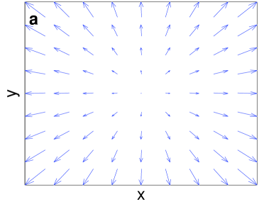
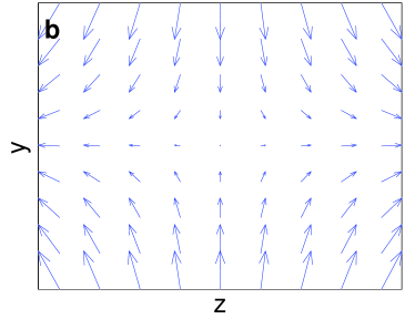
Figure 1: Vectorial plots of the magnetic quadrupole field (5). The intersections are the $(x,y)$-plane for $z=0$ (a) and the $(y,z)$-plane for $x=0$ (b).

Figure 1 shows intersections of this vector field for $z=0$ and $x=0$, correspondingly. A vector potential belonging to the quadrupole field reads

$$\vec{A}(\vec{r})=\frac{1}{3}\left[\vec{B}(\vec{r})\times\vec{r}\right]=b\left(\begin{array}[]{c}yz\\ -xz\\ 0\\ \end{array}\right),$$ (9)

which is a Coulomb gauge ($\nabla\vec{A}(\vec{r})=0$). In Cartesian coordinates and adopting atomic units ($g_{s}=2$) the spinor Hamiltonian (1) becomes

$${H_{C}}=-\frac{1}{2}\triangle-\frac{1}{\sqrt{x^{2}+y^{2}+z^{2}}}-b\,z{L}_{z}+\frac{b^{2}}{2}z^{2}\left(x^{2}+y^{2}\right)+\frac{b}{2}\left(\sigma_{x}x+\sigma_{y}y-2\sigma_{z}z\right)$$ (10)

with $L_{z}=-i\left(y\partial_{x}-x\partial_{y}\right)$ and $\sigma_{x}$, $\sigma_{y}$, $\sigma_{z}$ being the Pauli spin matrices ($\vec{S}=\frac{1}{2}\vec{\sigma}$). The first two terms of $H_{C}$ in equation (10) represent the Hamiltonian of the hydrogen atom without external fields. The third term is the paramagnetic ($\propto b$) or Zeeman-term. In contrast to the situation of the atom in a homogeneous field this term now depends not only on $L_{z}$ but also linearly on the $z$-coordinate. The fourth (diamagnetic) term ($\propto b^{2}$) represents a quartic oscillator coupling term between the cylindrical coordinates $\rho=\sqrt{x^{2}+y^{2}}$ and $z$. In a homogeneous field the diamagnetic interaction is a pure harmonic oscillator term proportional to $\rho^{2}$ and yields a confinement perpendicular to the magnetic field. Finally the reader should note that the coupling of the electronic spin to the quadrupole field depends linearly on the Cartesian coordinates. The latter prevents the factorization of the motions in the spin and spatial degrees of freedom and renders the corresponding Schrödinger equation into a spinor equation. This is again in contrast to the situation of a homogeneous magnetic field where the spin component along the field is a conserved quantity.

III Symmetries

In this section we investigate the unitary as well as the anti-unitary symmetries and conserved quantities of the Hamiltonian (10). We will then construct the corresponding eigenfunctions respecting these symmetries. This will help us (in Section 19) to derive properties of expectation values. Some basic definitions and features of probability densities are also introduced being utilized later to analyze excited atomic states in the quadrupole field.

For the following discussion it is useful to transform the Hamiltonian (10) into spherical coordinates. It reads

$${H_{S}} = -\frac{1}{2}\triangle_{r,\theta,\phi}-\frac{1}{r}+\frac{b^{2}}{2}r^{4}\cos^{2}\theta\sin^{2}\theta+\frac{b}{2}r\sin\theta\,K-b\,r\cos\theta\left({L}_{z}+\sigma_{z}\right)$$ (11)

with $K$ being the matrix

$$K=\left(\begin{array}[]{cc}0&e^{-i\phi}\\ e^{i\phi}&0\\ \end{array}\right).$$ (14)

As a consequence of the rotational invariance of the quadrupole field the $z$-component of the total angular momentum $J_{z}=L_{z}+S_{z}$ is conserved, i.e. we have $\left[H_{S},J_{z}\right]=0$. Additionally we have the discrete symmetry represented by the unitary operator $P_{\phi}OP_{z}$, i.e. $\left[H_{s},P_{\phi}OP_{z}\right]=0$. Here $O\equiv\sigma_{x}$ exchanges the components of a $\frac{1}{2}$-spinor, $P_{z}$ is the $z$-parity operator $P_{z}:z\rightarrow-z$ and $P_{\phi}$ represents the ’reflection’ $P_{\phi}:\phi\rightarrow 2\pi-\phi$. Apart from these symmetries the Hamiltonian possesses two generalized anti-unitary time reversal symmetries namely $TOP_{z}$ and $TP_{\phi}$. Both of them involve the conventional time reversal operator $T$ ($T^{2}=1$), which corresponds to complex conjugation. Applying the two anti-unitary operators $TOP_{z}$ and $TP_{\phi}$ results in the unitary operation $P_{\phi}OP_{z}$. The operators $TOP_{z}$, $TP_{\phi}$ and $P_{\phi}OP_{z}$ form an invariant Abelian sub-group. Together with $J_{z}$ they obey the following (anti-)commutation rules:

$$\left[J_{z},TP_{\phi}\right]=\left\{J_{z},TOP_{z}\right\}=\left\{J_{z},P_{\phi}OP_{z}\right\}=0$$ (15)

$$\left[TP_{\phi},TOP_{z}\right]=\left[TP_{\phi},P_{\phi}OP_{z}\right]=\left[P_{\phi}OP_{z},TOP_{z}\right]=0$$ (16)

Apparently the spin-spatial symmetry operations form a non-Abelian symmetry group. This group generated by $P_{\phi}OP_{z}$ and $J_{z}$ is isomorphic to $C_{\infty}\bigotimes C_{s}$.

In the following we will show, that the interplay of the above symmetries leads to a degeneracy of the eigenvalues of the Hamiltonian (11). We consider a state $\left|E,m\right>$ which is an eigenstate of the Hamiltonian (11) with the energy $E$ and to $J_{z}$ with the half-integer quantum number $m$ (see below). Since $TOP_{z}$ commutes with $H_{S}$ the state $TOP_{z}\,\left|E,m\right>$ is also an energy eigenstate with the energy $E$. By letting $J_{z}$ act on this state one obtains

$$J_{z}\,TOP_{z}\,\left|E,m\right>=-TOP_{z}\,J_{z}\,\left|E,m\right>=-m\,TOP_{z}\,\left|E,m\right>.$$

Thus the state $TOP_{z}\,\left|E,m\right>$ can be identified with $\left|E,-m\right>$. Hence the states with the eigenvalues $m$ and $-m$ are degenerate. This two-fold degeneracy of each energy level in the presence of the inhomogeneous magnetic field is a remarkable feature. It is reminiscent of the Kramers degeneracy of spin $\frac{1}{2}$ systems in the absence of external fields Haake01 .

In the case of an atom in a homogeneous magnetic field the operators $L_{z}$, $P_{z}$ as well as parity $P$ and $T\sigma_{z}P_{\phi}$ form the corresponding set of spatial and time reversal symmetries if the field is oriented along the $z$-axis. Since these operators commute they form an Abelian symmetry group implying the well-known fact that there are no energy level degeneracies in the homogeneous field.

In order to finalize this section we want to remark that most of the above considerations hold not only for the case of a fixed nucleus in the trap center but also for the full two-body problem. If the dynamics of both the nucleus and the electron is considered the conservation of $TP_{\phi}$, $TOP_{z}$ and $J_{z}$ of the two-body system holds.

IV $J_{z}$-, $TOP_{z}$- and $TP_{\phi}$-eigenstates

Since the $J_{z}$ operator provides the eigenvalue equation $J_{z}\left|m\right>=m\,\left|m\right>$ with half-integer $m$ the spatial representation of the spinor eigenfunctions $\left|m\right>$ are

$$\left|m\right>=\left(\begin{array}[]{c}e^{i(m-\frac{1}{2})\phi}\\ e^{i(m+\frac{1}{2})\phi}\\ \end{array}\right).$$ (19)

The eigenfunction $\left|m\right>$ can be used to reduce the electron dynamics to a given $m$-subspace. The quantized motion of the electron is then described by the Hamiltonian $H_{m}=\left<m\right|H\left|m\right>$. We will exploit this fact later when solving the stationary Schrödinger equation.

Eigenstates to the $TOP_{z}$-operator can be constructed by superimposing two degenerate $J_{z}$-eigenstates. They read

$$\left|E,\pm\right>^{TOP_{z}}=\frac{1}{\sqrt{2}}\left[\left|E,m\right>\pm TOP_{z}\,\left|E,m\right>\right].$$ (20)

The corresponding eigenvalue relation is

$$TOP_{z}\,\left|E,\pm\right>=\pm\left|E,\pm\right>.$$ (21)

Eigenfunctions of the anti-unitary operator $TP_{\phi}$ can be constructed analogously:

$$\left|E,\pm\right>^{TP_{\phi}}=\frac{1}{\sqrt{2}}\left[\left|E,m\right>\pm TP_{\phi}\,\left|E,m\right>\right]$$ (22)

The $J_{z}$- and $TOP_{z}$-eigenstates exhibit certain symmetry properties. Exploiting such symmetries often turns out to be extremely powerful and can save a lot of computational effort. It is especially useful when one is interested in computing matrix elements such as expectation values of certain observables.

The expectation value of an observable $M$ in an energy and $J_{z}$- eigenstate $\left|E,m\right>$ is defined as $\left<M\right>_{J_{z}}=\left<E,m\right|M\left|E,m\right>$ whereas for a $TOP_{z}$-eigenstate (20) it reads

$$\left<M\right>^{\pm}_{TOP_{z}} = {{}^{TOP_{z}}}\left<E,\pm\right|M\left|E,\pm\right>^{TOP_{z}}$$ (23)

$$= \frac{1}{2}\left[\left<M\right>_{J_{z}}+\left<TOP_{z}\,M\,TOP_{z}\right>_{J_{z}}\pm\left<TOP_{z}\,M\right>^{*}_{J_{z}}\pm\left<M\,TOP_{z}\right>_{J_{z}}\right].$$

If $M$ satisfies the anti-commutation relation $\left\{TOP_{z},M\right\}=0$ the first two terms of (23) cancel each other and we obtain

$$\left<M\right>^{\pm}_{TOP_{z}}=\pm\frac{1}{2}\left[\left<TOP_{z}\,M\right>^{*}_{J_{z}}-\left<TOP_{z}\,M\right>_{J_{z}}\right]=\mp i\,\text{Im}\left(\left<TOP_{z}\,M\right>_{J_{z}}\right).$$ (24)

Since the expectation value of an observable is always a real number it follows

$$\left<M\right>^{\pm}_{TOP_{z}} = 0,$$ (25)

i.e. the expectation value of such an operator $M$ vanishes within any $TOP_{z}$-eigenstate.

In a similar manner one can calculate the expectation value of an observable $N$, which commutes with $J_{z}$ and $TOP_{z}$. Here expression (23) yields

$$\left<N\right>^{\pm}_{TOP_{z}}=\left<N\right>_{J_{z}}\pm\left<N\,TOP_{z}\right>_{J_{z}}.$$ (26)

Exploiting $\left[N,J_{z}\right]=0$ and using $\left\{TOP_{z},J_{z}\right\}=0$ one obtains

$$\left<N\,TOP_{z}\right>_{J_{z}} = \frac{1}{m}\left<E,m\right|N\,TOP_{z}\,J_{z}\left|E,m\right>=-\frac{1}{m}\left<E,m\right|N\,J_{z}\,TOP_{z}\left|E,m\right>$$ (27)

$$= -\frac{1}{m}\left<E,m\right|J_{z}\,N\,TOP_{z}\left|E,m\right>=-\left<N\,TOP_{z}\right>_{J_{z}}$$

Hence $\left<N\,TOP_{z}\right>_{J_{z}}=0$ leading to the final result

$$\left<N\right>^{\pm}_{TOP_{z}}=\left<N\right>_{J_{z}},$$ (28)

i.e. we obtain equal expectation values of $N$ for a $J_{z}$- or $TOP_{z}$-eigenstate.

Finally we provide some relevant expressions for the spatial probability density $W$ in the different representations. The probability density belonging to the $J_{z}$-eigenstate $\left|E,m\right>=\left|u\right>\left|\uparrow\right>+\left|d\right>\left|\downarrow\right>$ reads

$$W_{J_{z}}\left(r,\theta,\phi\right)=r^{2}\sin\theta\left[\left|u\left(r,\theta\right)\right|^{2}+\left|d\left(r,\theta\right)\right|^{2}\right].$$ (29)

Since the whole $\phi$-dependence is contained in phase-factors (see eq. (19)) $W_{J_{z}}$ is invariant under rotations around the $z$-axis. For the $TOP_{z}$-eigenstates (20) one obtains

$$W_{TOP_{z}}\left(r,\theta,\phi\right) = \frac{r^{2}\sin\theta}{2}\left[\left|u\left(r,\theta\right)\right|^{2}+\left|d\left(r,\theta\right)\right|^{2}+\left|u\left(r,\pi-\theta\right)\right|^{2}+\left|d\left(r,\pi-\theta\right)\right|^{2}\right.$$

$$\left.\pm 2\,\left\{u\left(r,\theta\right)d\left(r,\pi-\theta\right)+d\left(r,\theta\right)u\left(r,\pi-\theta\right)\right\}\cos\left(2m\,\phi\right)\right].$$

$W_{TOP_{z}}\left(r,\theta,\phi\right)$ is constructed from $TOP_{z}$-eigenstates and obeys therefore the $TOP_{z}$-symmetry. Since $W_{TOP_{z}}\left(r,\theta,\phi\right)$ is a real scalar function the symmetries $T$ and $O$ are trivially satisfied leading to

$$W_{TOP_{z}}=TOP_{z}\,W_{TOP_{z}}\,(TOP_{z})^{-1}=TP_{z}\,W_{TOP_{z}}\,(TP_{z})^{-1}=P_{z}\,W_{TOP_{z}}\,(P_{z})^{-1},$$ (31)

showing that $W_{TOP_{z}}\left(r,\theta,\phi\right)$ is invariant under $z$-parity.

V Computational approach

We employ the linear variational principle Szabo96 to find the eigenvalues and eigenvectors of the Hamiltonian (11). The idea is to expand the exact eigenfunctions of the Schrödinger equation in a complete basis set of spinor orbitals that converge efficiently and accurately towards the exact solution. Calculating the expansion coefficients results in a large-scale algebraic eigenvalue equation.
The basis set $\left\{B^{\uparrow}_{nl},B^{\downarrow}_{\tilde{n}\tilde{l}}\right\}_{m}$ we apply for given $m$ takes the following form for the upper and lower component, respectively:

$$\left<r,\theta,\phi\mid B^{\uparrow}_{nl}\right>=R_{n}^{(\zeta,k)}(r)Y_{l}^{m-\frac{1}{2}}(\theta,\phi)\left|\uparrow\right>\quad,\quad\left<r,\theta,\phi\mid B^{\downarrow}_{\tilde{n}\tilde{l}}\right>=R_{\tilde{n}}^{(\zeta,k)}(r)Y_{\tilde{l}}^{m+\frac{1}{2}}(\theta,\phi)\left|\downarrow\right>$$ (32)

Here $Y_{l}^{m}(\theta,\phi)$ denote the spherical harmonics. Due to the appearance of the upper and lower spinor orbitals for fixed $m$ the energy eigenfunctions of the Schrödinger equation computed with this basis set are a priori eigenfunctions of $J_{z}$.

The radial part of the orbitals used for the expansion reads

$$R_{n}^{(\zeta,k)}(r)=\sqrt{\frac{n!}{(n+2k)!}}e^{-\frac{\zeta r}{2}}(\zeta r)^{k}L_{n}^{2k}(\zeta r)$$ (33)

with $L_{n}^{2k}(r)$ being the Laguerre polynomials. The parameters $k$ and $\zeta$ can be tuned to optimize the convergence behavior in different parts of the spectrum. $\zeta$ possesses the dimension of an inverse length. In order to converge eigenstates with the smallest possible number of basis functions $1/\zeta$ has to be adapted for every energy regime such, that it corresponds to the typical spatial extensions of the wavefunctions. For fixed $k$ and $\zeta$ the functions $R_{n}^{(\zeta,k)}(r)$ form a complete functional set in $r$-space but are non-orthogonal leading to a non-trivial overlap-matrix. The basis set (32) is complete in $r$-, $\theta$- and spin-space.

An eigenstate $\left|E,m\right>$ of the stationary Schrödinger equation can now be expanded in terms of the basis-functions (32)

$$\left|E,m\right> = \sum_{n=0,l=\left|m-\frac{1}{2}\right|}^{n<N,l<L}a_{n,l}\left|B^{\uparrow}_{nl}\right>+\sum_{\tilde{n}=0,\tilde{l}=\left|m+\frac{1}{2}\right|}^{\tilde{n}<\tilde{N},\tilde{l}<\tilde{L}}b_{\tilde{n},\tilde{l}}\left|B^{\downarrow}_{\tilde{n}\tilde{l}}\right>$$ (34)

leading to the generalized spinor eigenvalue problem $\mathbf{H}\vec{c}=E\mathbf{S}\vec{c}$, where $\mathbf{H}$ and $\mathbf{S}$ are the corresponding matrix representation of the Hamiltonian (11) and the overlap matrix, respectively:

$$\mathbf{H}=\left(\begin{array}[]{cc}\left<B^{\uparrow}_{nl}\left|{H}\right|B^{\uparrow}_{n^{\prime}l^{\prime}}\right>&\left<B^{\uparrow}_{nl}\left|{H}\right|B^{\downarrow}_{\tilde{n}^{\prime}\tilde{l}^{\prime}}\right>\\ \left<B^{\downarrow}_{\tilde{n}\tilde{l}}\left|{H}\right|B^{\uparrow}_{n^{\prime}l^{\prime}}\right>&\left<B^{\downarrow}_{\tilde{n}\tilde{l}}\left|{H}\right|B^{\downarrow}_{\tilde{n}^{\prime}\tilde{l}^{\prime}}\right>\\ \end{array}\right)\quad\mathbf{S}=\left(\begin{array}[]{cc}\left<B^{\uparrow}_{nl}\mid B^{\uparrow}_{n^{\prime}l^{\prime}}\right>&0\\ 0&\left<B^{\downarrow}_{\tilde{n}\tilde{l}}\mid B^{\downarrow}_{\tilde{n}^{\prime}\tilde{l}^{\prime}}\right>\\ \end{array}\right)$$ (39)

The vector $\vec{c}$ contains the expansion coefficients of (34):

$$\vec{c}=\left(\begin{array}[]{c}a_{n,l}\\ b_{\tilde{n},\tilde{l}}\\ \end{array}\right)$$ (42)

The two off-diagonal blocks of $\mathbf{S}$ vanish due to the orthogonality of the spin states $\left|\uparrow\right>$ and $\left|\downarrow\right>$. This does not hold for $\mathbf{H}$ since the magnetic field leads to a coupling of the two spinor components. With the basis set (32) all entries of the matrices (39) can be computed analytically. To do this we have exploited recurrence identities for the spherical harmonics and the Laguerre polynomials Abramowitz68 . The matrices $\mathbf{H}$ and $\mathbf{S}$ possess a particular sparse appearance, e.g. $\mathbf{S}$ is penta-diagonal, enabling us to go to large basis set dimensions.

In order to solve the above generalized eigenvalue problem we employ the Arnoldi-method Sorensen which is a so-called Krylov-space method. This approach is especially suited for eigenvalue equations involving large sparse matrices. The Arnoldi-Method is perfectly suited to provide low-lying excited states with fairly small basis sets. To calculate highly excited states without computing the lower excited states we use the so called shift-and-invert method. Here the generalized eigenvalue problem is transformed to $\left(\mathbf{H}-\sigma\,\mathbf{S}\right)^{-1}\mathbf{S}\vec{c^{\prime}}=\lambda\vec{c^{\prime}}$. The eigenvalues $E$ of the original eigenvalue equation are connected to $\lambda$ according to $E_{i}=\sigma+\frac{1}{\lambda}$. Thus eigenvalues lying close to the shift $\sigma$ become the largest eigenvalues in magnitude of the operator $\left(\mathbf{H}-\sigma\,\mathbf{S}\right)^{-1}\mathbf{S}$. Using the Arnoldi-method these eigenvalues lying in a predefined energy range of the spectrum will converge first. The shift-and-invert method allows in principle to compute arbitrary parts of the spectrum of the Hamiltonian (11) by resetting the shift $\sigma$ in successive calculations. Thereby the basis parameter $\zeta$ has to be adapted. A good choice is $\zeta=\frac{2\sqrt{\left|E\right|}}{0.775}$ where $E$ is the lower boundary of the corresponding energy range. We remark that there is no need to change the parameter $k$, which we always put to zero.

Due to the Hylleraas-Undheim theorem Newton82 the numerical approximate eigenvalues provide an upper bound for the exact eigenvalues. In order to check the convergence behavior we calculate a number of eigenvalues $E_{i}^{G_{1}}$ for a given basis set size $G_{1}$. In a second step the size of the basis set is increased significantly to $G_{2}$ and the same eigenvalues are calculated again being now denoted by $E_{i}^{G_{2}}$. As a measure of convergence we define the quantity

$$K_{i}=\left|\frac{E_{i}^{G_{1}}-E_{i}^{G_{2}}}{E_{i}^{G_{1}}-E_{i-1}^{G_{1}}}\right|$$ (43)

where the difference of the same eigenvalue for the two basis sizes $G_{1}$ and $G_{2}$ is divided by the distance to the lower neighboring eigenvalue. For $K_{i}\leq 0.01$ we assume the eigenvalue $E_{i}^{G_{2}}$ to be well converged.

The maximum dimension of the basis sets we employed was approximately 17000. We thereby were able to converge several thousand eigenstates and eigenvalues up to energies corresponding to a hydrogen principle quantum number of $n\approx 60$ for weak gradients and gradients $b$ ranging from $10^{-10}$ to $10$ covering the $J_{z}$-quantum numbers $m\,\epsilon\,\left[-\frac{7}{2},\frac{7}{2}\right]$.

VI Results

In the following we discuss and analyze our results on the atom in the quadrupole field. We address for different regimes of the field gradient the effects of the quadrupole field on the spatial appearance of the wavefunctions as well as their spin properties. Furthermore we provide the selection rules for electric dipole transitions. A comparison with properties of the atom in a homogeneous magnetic field is performed to illuminate the specific features in a quadrupole field.

VI.1 Spectral Properties

Depending on the gradient $b$ of the quadrupole field one can distinguish three regimes: the weak, the intermediate and the strong gradient regime. In each of these regimes the atoms exhibits unique features. The notion of a weak/strong gradient does not refer to an absolute field gradient but depends on the degree of excitation of the atom. It is defined to be the regime, for which the magnetic compared to the Coulomb interaction is weak/strong. For weak gradients the level structure is dominated by the spin as well as the spatial Zeeman-term both of which depend linearly on the field gradient. The level degeneracies at $b=0$ are lifted and a linear splitting of the $n$-multiplets is observed. There is no overlap between neighboring $n$-multiplets which renders $n$ an approximately good quantum number.

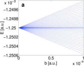
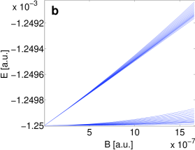
Figure 2: a: Energy level splitting of the $m=\frac{1}{2}$-states of the $n=20$-multiplet in the quadrupole field. b: Splitting of the same energies in a homogeneous field.

Figure 2a shows the linear splitting of the $n=20$ multiplet for the states with quantum number $m=\pm\frac{1}{2}$. The levels are arranged symmetrically around the energy for zero field. This is in contrast to the level splitting of an atom in a homogeneous magnetic field which is presented in figure 2b for the same $n$-multiplet. Here the Zeeman-terms cause a linear energetical splitting into only two branches. The latter (for fixed $m$) is the result of the two possible spin orientations in a homogeneous magnetic field. In a quadrupole field $L_{z}$ and $S_{z}$ are not conserved separately and an assignment of spin orientations is therefore not possible.

With increasing gradient the diamagnetic term with its quadratic dependence on $b$ (or $B$ in the homogeneous field) becomes increasingly important thereby resulting in a non-linear behavior of the energy curves. The intra $n$-manifold mixing regime where different $n$-multiplets are still energetically well separated but different angular momentum states ($l$-states) mix can be shown to scale as $b\propto n^{-6}$. In the high gradient regime different $n$-multiplets begin to overlap and avoided crossings dominate the spectra.

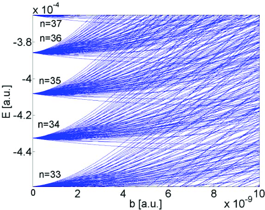
Figure 3: Energy spectrum of the multiplets $n=33-37$ for the states with $m=\pm\frac{1}{2}$. For low gradients the energy levels split almost linearly followed by a transition region where the diamagnetic term becomes increasingly more important. For high gradients different $n$-multiplets overlap and no symmetries, i.e. approximate quantum numbers, are left.

The onset of this inter $n$-manifold mixing scales according to $b\propto n^{-\frac{11}{2}}$ whereas in the homogeneous field the scaling is $B\propto n^{-\frac{7}{2}}$. Figure 3 shows the energy levels of $n$-multiplets ranging from $n=33$ to $n=37$ with $m=\pm\frac{1}{2}$ in the regime $0\leq b\leq 10^{-8}$. For such a degree of excitation the intra $n$-manifold mixing sets in at $b\approx 5\cdot 10^{-10}$. Therefore the linear splitting due to the Zeeman-term as shown in figure 2 is hardly visible.

VI.2 Low lying states and large gradients

Although gradients $b\gg 10^{-10}$ are not experimentally accessible it is at this point instructive to illuminate their impact on low-lying electronic states. This way some principle features of the influence of the quadrupole field on the electronic structure of the atom will become clear.

Here we consider the behavior of the lowest three $n$-multiplets as a function of $b$ for $0<b<10^{-2}$ (see figure 4).

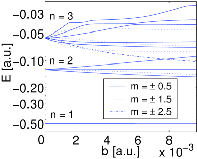
Figure 4: Energy level structure of the three lowest $n$-multiplets. The $J_{z}$ quantum number ranges from $-\frac{5}{2}$ to $\frac{5}{2}$.

The splitting of the $n=3$ multiplet is linear up to $b=5\cdot 10^{-4}$, where inter $n$-manifold mixing begins.

The kink of the energetically highest-lying curve at $b=2\cdot 10^{-3}$ is the result of an avoided crossing with an energy level from the upper $n=4$ multiplet. Moving to higher gradients we encounter further avoided crossing. Crossings between levels belonging to different quantum numbers $m$ are exact, since the corresponding states belong to separate symmetry sub-spaces. The $n=2$ multiplet does not show any indication of inter $n$-manifold mixing throughout the whole gradient range considered here. Figure 4 shows also that the energy of the degenerate ground state depends very weakly on the gradient $b$: We observe a maximum relative energy shift of about $0.04\%$ at $b=10^{-2}$.

VI.3 Radial compression of the wavefunctions

The operator $r$ obeys the commutators $\left[r,TOP_{z}\right]=0$ and $\left[r,J_{z}\right]=0$. Together with (28) this yields

$$\left<r\right>=\left<r\right>^{\pm}_{TOP_{z}}=\left<r\right>_{J_{z}}.$$ (44)

Thus the expectation value of $r$ in the $J_{z}$ eigenstates is the same as in the $TOP_{z}$-eigenstates.
For the one-electron problem without external field we have $\left<r\right>^{H}=\frac{1}{2}\left(3n^{2}-l(l+1)\right)$. Since $l$ satisfies $0\leq l\leq n-1$ one obtains corresponding upper and lower bounds for the expectation value of $r$: $n\left(n+\frac{1}{2}\right)\leq\left<r\right>^{H}\leq\frac{3}{2}n^{2}$. In figure 5 this expectation value is shown for the atom in the quadrupole field as a function of the principle quantum number $n$ for two different gradients ($n$ serves here as a label for the energy levels and is not a good quantum number!).

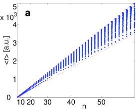
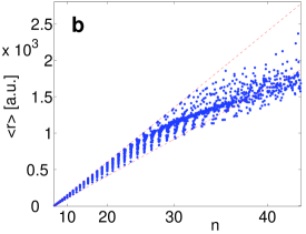
Figure 5: Expectation value of the radial coordinate $r$ plotted against the principle quantum number $n$ at different gradients (a: $b=10^{-10}$, b: $b=10^{-8}$).

The radial expectation values lie in between the boundaries given by the field-free inequality indicated by the dashed lines (see figure 5a). Expectation values of states belonging to the same $n$-multiplet are arranged in vertical lines expressing their energetical degeneracy (see figure 5a for $b=10^{-10}$). Here states with large expectation values of $r$ possess small expectation values of the angular momentum and vice versa. The situation is different for $b=10^{-8}$. Here a systematic decrease of the $r$-expectation values takes place for states with an energy corresponding to $n>30$. This is also the energy regime where the inter $n$-manifold mixing sets in. Here the mentioned pattern of vertical lines dissolves and a irregular looking distribution emerges. Although the expectation values are not located between the dashed boundaries the distribution is still widespread which can be ascribed to the different angular momentum distribution of the states.

We now investigate the deformation of the ground state wavefunction in both the quadrupole and the homogeneous field. Due to their simple nodal structure they are suited best to point out differences arising for the two different field configurations. To demonstrate the deformation effects on the electronic cloud we consider for reasons of illustration an extremely high gradient.

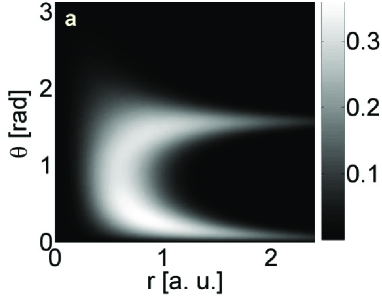
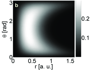
Figure 6: Spatial probability density of the ground state in the quadrupole field (a) and a homogeneous field pointing in the $z$-direction (b) for $b=B=10$ and $m=\frac{1}{2}$.

Figure 6 shows the spatial probability density of the ground state in the quadrupole field (6a) at $b=10$ and the homogeneous field (6b) at $B=10$ ($m=\frac{1}{2}$ in both cases).

For the quadrupole field we observe an asymmetric deformation with respect to the $\theta=\frac{\pi}{2}$-plane: the electronic wavefunction is almost completely confined to the upper half-volume ($\theta<\frac{\pi}{2}$) which is a consequence of the symmetries discussed in section III: $z$-parity is not conserved and eigenstates appear in pairs one being the mirror image of the other with respect to the reflection at the $x-y$-plane. Furthermore we observe that the electronic motion is localized particularly along the two ’channels’ for $\theta=0$ corresponding to the lower $z$-axis and $\theta=\frac{\pi}{2}$ being the $x-y$-plane. This property as well as the detailed shape of the electronic probability density in the individual half-volume is determined by the diamagnetic term which is dominant in the high gradient regime. For the quadrupole field it is proportional to $\sin^{2}\theta\cos^{2}\theta$ reaching its maximum value at $\theta=\frac{\pi}{4},\frac{3\pi}{4}$. The probability density in a homogeneous field (see figure 6b) exhibits the above-mentioned corresponding reflection symmetry due to the invariance of the corresponding Hamiltonian with respect to $z$-parity. Here we observe the maximum of the probability density at $\theta=\frac{\pi}{2}$ and a deformation towards $\theta=\pi$ and $\theta=0$ leading to a cigar-like shape. The diamagnetic term is proportional to $\sin^{2}\theta$ having its maximum value at $\theta=\frac{\pi}{2}$ thus coinciding with the regions possessing the strongest deformation of the probability density. For both field configurations the probability density vanishes at $r=0$. The maximum is reached at $r\approx 0.75$ in the quadrupole field and for $r\approx 0.5$ in the homogeneous field followed by an exponential drop-off.

VI.4 Properties of the electronic spin

VI.4.1 Expectation values

In a homogeneous magnetic field the projection of the spin operator onto the direction of the magnetic field is a conserved quantity. In this case one can choose the energy eigenstates to be also eigenfunctions with respect to $S_{z}$. This restricts $\left<S_{z}\right>$ to the two values $\pm\frac{1}{2}$. In the quadrupole field $S_{z}$ is not conserved, and we therefore consider the expectation value $\left<S_{z}\right>$ of the electronic states. We have

$$\left<S_{z}\right>_{J_{z}}=\frac{1}{2}\left[\left<u\mid u\right>-\left<d\mid d\right>\right].$$ (45)

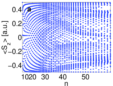
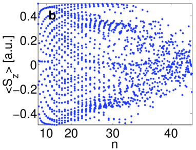
Figure 7: Expectation values of the $z$-component of the spin operator as a function of the quantum number $n$ for different gradients (a: $b=10^{-10}$, b: $b=10^{-8}$).

Figure 7 shows the distribution of $\left<S_{z}\right>_{J_{z}}$ for electronic states of the $m=\frac{1}{2}$ subspace as a function of the principle quantum number $n$. Since $S_{z}$ is not conserved the values of $\left<S_{z}\right>$ are allowed to cover the complete interval $\left[-\frac{1}{2},\frac{1}{2}\right]$. For $b=10^{-10}$ (figure 7a) and a low degree of excitation the expectation values are evenly distributed over the interval. When reaching highly excited states this pattern becomes increasingly distorted. The expectation values agglomerate at $-0.35$ and $0.35$ for $n\geq 50$. Due to the approximate degeneracy of the energy levels at low energies, i.e. small $n$, the values of $\left<S_{z}\right>$ form vertical lines. These lines widen for higher $n$. Since at $b=10^{-10}$ no significant $n$-mixing up to our maximum converged energy levels takes place, neighboring lines are well separated. For a higher gradient $b=10^{-8}$ (figure 7b) the above properties are equally present for low-lying states. However, with increasing excitation energy we now observe a complete $n$-mixing regime where the regular patterns disappear and we obtain an irregular distribution of $\left<S_{z}\right>$. Overall the distribution narrows, e.g. for $n=40$ the occupied interval is approximately $\left[-0.3,0.3\right]$.

We remark that due to the fact that the $S_{z}$-operator anti-commutes with $TOP_{z}$ we have $\left<S_{z}\right>_{TOP_{z}}^{\pm}=0$. Apparently there is no preferred direction for the electronic spin in a state obeying the $TOP_{z}$ symmetry.

VI.4.2 Spin polarization

Due to the coupling of the spatial to the spin degrees of freedom we have to expect a dependence of the spin orientation on the spatial coordinates. To investigate this in more detail we study the spatially dependent $S_{z}$-polarization $W_{S}(\vec{r})$. For a $J_{z}$-eigenstate $\left|E,m\right>$ it reads

$$W_{S}(\vec{r}) = \frac{\left<E,m\mid\vec{r}\right>{S}_{z}\left<\vec{r}\mid E,m\,\right>}{\left<E,m\mid\vec{r}\right>\left<\vec{r}\mid E,m\,\right>}=\frac{1}{2}\frac{\left|\left<u\mid\vec{r}\right>\right|^{2}-\left|\left<d\mid\vec{r}\right>\right|^{2}}{\left|\left<u\mid\vec{r}\right>\right|^{2}+\left|\left<d\mid\vec{r}\right>\right|^{2}}.$$ (46)

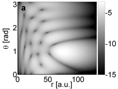
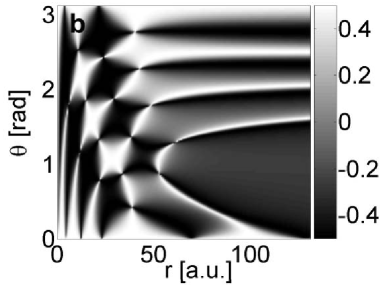
Figure 8: a: Spatial probability density of the $45th$ excited state for $m=\frac{1}{2}$ and $b=10^{-8}$ in logarithmic representation. b: $S_{z}$-polarization for the same state.

Figure 8 shows the spatial probability distribution (8a) and the $S_{z}$-polarization (8b) for the $45th$ excited state for $m=\frac{1}{2}$ and $b=10^{-8}$ emerging from the $n=7$ multiplet at $b=0$. The probability density is shown for a logarithmic scale to provide details for small values. In contrast to the constant $S_{z}$-polarization we would encounter in the absence of a field or a homogeneous field we observe a complex pattern of domains exhibiting different spin orientation (white: spin up, black: spin down). At low $r$ values these domains form a pattern similar to that of a chess board. With increasing $r$ a transition region is encountered where the formation of stripes with different spin orientation begins. The junctions where four spin domains meet each other coincide with the nodes of the spatial probability density. The Coulomb interaction as well as the spin-Zeeman term are responsible for the interwoven network of island of different spin orientation. The additional presence of the orbital Zeeman and the diamagnetic term leads to a deformation of this network.

Highly excited states, i.e. Rydberg states, typically possess a large spatial extension. In figure 9 the spatial probability density (9a) and the $S_{z}$-polarization (9b) are depicted for the $1117th$ excited state of the $m=\frac{1}{2}$ subspace ($b=10^{-8}$). At small $r$-values the $S_{z}$-polarization shows the chess board pattern, we have already observed for the low-lying excited states, followed by a striped region.

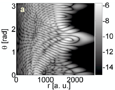
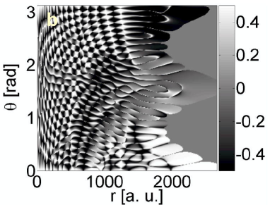
Figure 9: Spatial probability density (a) and $S_{z}$-polarization (b) for the $1117th$ excited state for $m=\frac{1}{2}$ and $b=10^{-8}$. At large $r$ the $S_{z}$-polarization becomes similar to $W_{S}^{+}$ indicating an antiparallel alignment of the electronic spin to the magnetic field.

Whereas for low radii the spin orientation changes locally from island to island generating an appealing pattern we observe an overall tendency of the electronic spin polarization in the region characterized by stripes ($r\approx 2000$). Here, independently of the nodal structure, the spin orientation changes smoothly from downwards at $\theta=\pi$ to upwards at $\theta=0$. This feature can be understood by inspecting the spin Zeeman term only. The corresponding Hamiltonian reads

$$\hat{H}_{S} = -\vec{\mu}\,\vec{B}(\vec{r})=\frac{b}{2}r\left(\begin{array}[]{cc}-2\,\cos\theta&\sin\theta\,e^{-i\phi}\\ \sin\theta\,e^{i\phi}&2\,\cos\theta\\ \end{array}\right).$$ (49)

Here the complete dynamics takes place in spin space since the spatial coordinates $\left(r,\theta,\phi\right)$ are entering as parameters. The eigenvalue problem belonging to (49) possesses the two solutions

$$\Phi_{\pm}(r,\theta,\phi)=\left(\begin{array}[]{c}-\frac{2\,\cos\theta\pm\sqrt{1+3\,\cos^{2}\theta}}{\sin\theta}e^{-i\phi}\\ 1\\ \end{array}\right)$$ (52)

with the energies

$$E_{\pm}=\mp\frac{1}{2}b\,r\sqrt{1+3\cos^{2}\theta}=\mp|\vec{\mu}||\vec{B}(\vec{r})|.$$ (53)

These energies correspond to those of a spin oriented parallel ($E_{-}$) or antiparallel ($E_{+}$) to the magnetic quadrupole field. Constructing the $S_{z}$-polarization $W_{S}^{\pm}$ of the eigenstates (53) yields

$$W_{S}^{\pm}=\frac{1}{2}\frac{(2\cos\theta\pm\sqrt{1+3\,\cos^{2}\theta})^{2}-\sin^{2}\theta}{(2\cos\theta\pm\sqrt{1+3\,\cos^{2}\theta})^{2}+\sin^{2}\theta}.$$ (54)

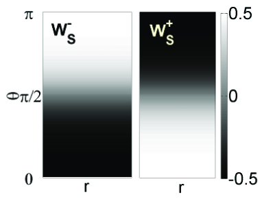
Figure 10: $S_{z}$-polarization of the two eigenstates of the Hamiltonian (49). The electronic spin either points parallel ($W_{S}^{-}$) or antiparallel ($W_{S}^{+}$) in the local direction of the field.

Both $W_{S}^{+}$ and $W_{S}^{-}$ are shown in figure 10. They do not depend on the radial coordinate and the azimuthal angle $\phi$. The $z$-component of the spin is oriented upwards/downwards at $\theta=0$ and points in the opposite direction at $\theta=\pi$. For $\theta=\frac{\pi}{2}$ there is a transition region with $W_{S}^{\pm}$ being close to zero.

This is precisely the above-discussed behavior we observe at large $r$ for the $S_{z}$-polarization of the Rydberg state depicted in figure 9b. Apparently in this special state the electron spin prefers an antiparallel alignment to the external field at large radii which corresponds to $W_{S}^{+}$. We remark that similar results on the spatial spin polarization are obtained if one considers the quantity $\vec{S}\vec{B}(\vec{r})$ instead of $S_{z}$.

VI.5 Electromagnetic transitions

The interaction of an atom in the magnetic field with external electromagnetic radiation leads to transitions among its electronic states which we describe employing the dipole approximation. The amplitude for a transition from the initial state $\left|i\right>$ to the final state $\left|f\right>$ is given by the matrix element $p_{if}^{\sigma^{\pm},\pi}=\left<i\right|D_{\sigma^{\pm},\pi}\left|f\right>$. Considering $\pi$ and $\sigma^{\pm}$ transitions the operator takes the common forms $D_{\pi}=z=r\cos\theta$ and $D_{\sigma^{\pm}}=\frac{1}{\sqrt{2}}\left(x\pm iy\right)=\frac{1}{\sqrt{2}}r\sin\theta e^{\pm i\phi}$, respectively. The symmetries of the $J_{z}$ and $TOP_{z}$ eigenstates result in selection rules which we will discuss in the following.

Evaluating the transition matrix element for $\pi$-transitions $\left<E^{\prime},m^{\prime}\right|r\cos\theta\left|E,m\right>$ leads to the selection rule $m^{\prime}-m=0$. For $\sigma^{\pm}$-transitions the corresponding matrix element reads $\left<E^{\prime},m^{\prime}\right|r\sin\theta\,e^{\pm i\phi}\left|E,m\right>$ which is only non-zero if $m^{\prime}-m=\pm 1$. Hence, electromagnetic transition between $J_{z}$ states occur only if $\triangle m=0,\pm 1$ reminiscent of the situation in a homogeneous or even no magnetic field. The corresponding matrix element for $\pi$-transitions between $TOP_{z}$-eigenstates is $\left<E^{\prime},\Pi^{\prime}\right|r\cos\theta\left|E,\Pi\right>$ leading to the selection rule $\Pi^{\prime}\neq\Pi$, i.e. only transitions between states with opposite $TOP_{z}$ symmetry are allowed. There are no selection rules for $\sigma^{\pm}$-transitions between $TOP_{z}$-eigenstates. The selection rules are summarized in table 1.

	$J_{z}-states$	$TOP_{z}-states$
transition type	$\triangle m=m^{\prime}-m$	$\triangle\Pi=\Pi^{\prime}-\Pi$
$\pi$	0	$\pm 2$
$\sigma^{+}$	1	-
$\sigma^{-}$	-1	-

Table 1: Selection rules for dipole transitions between $J_{z}$-eigenstates and between $TOP_{z}$-eigenstates.

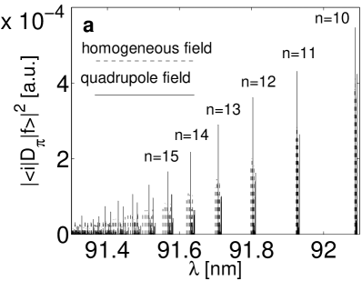
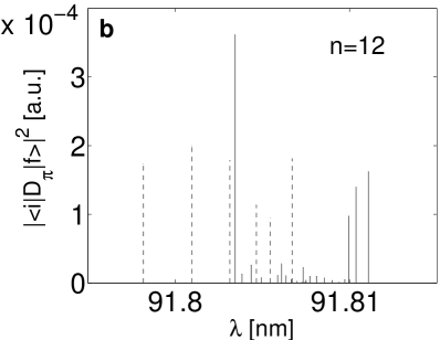
Figure 11: Dipole strengths of $\triangle m=0$ $\pi-$transitions from the ground state to excited levels. Solid lines denote transitions in the quadrupole field whereas transitions in the homogeneous field are indicated by dashed lines. a: The line possessing the largest wavelength belongs to the $n=1\rightarrow 10$ transition. b: Magnification of the line structure of the $n=1\rightarrow 12$ transitions.

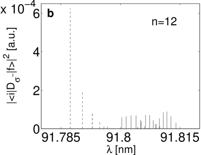
Figure 12: Dipole strengths of $\triangle m=-1$ $\sigma-$ transitions ($\sigma^{-}$-transitions) from the ground state to excited levels. Solid lines denote transitions in the quadrupole field whereas transitions in the homogeneous field are indicated by dashed lines. a: The line possessing the lowest wavelength belongs to the $n=1\rightarrow 10$ transition. b: Magnification of the line structure of the $n=1\rightarrow 12$ transition.

We have calculated the dipole strengths for transitions from the ground state ($m=\frac{1}{2}$) to excited states with $m=\frac{1}{2}$ ($\pi$-transitions (figure 11)) and $m=\frac{3}{2}$ ($\sigma^{-}$-transitions (figure 12)). For comparison we also present the transitions for an atom in a homogeneous magnetic field indicated by dashed lines whereas transitions in the quadrupole field are represented as solid lines. For a detailed discussion of electromagnetic transitions in the homogeneous field we refer the reader to Ruder94 ; Clark80 ; Clark82 . In order to make both results comparable we have chosen the gradient and the magnetic field strength such that we observe approximately equal splitting of the $n$-multiplets with increasing energy. Specifically we chose $b=10^{-7}$ and $B=10^{-4}$. Figure 11a shows the dipole strengths for $\pi$-transitions. Here the line possessing the largest wavelength emerges from the transition to the $n=10$ multiplet which already exhibits significant features of intra $n$-manifold mixing. From here up to a certain wavelength ($\approx 91.5nm$) neighboring lines are well separated. Transitions with smaller wavelengths involve levels showing inter $n$-manifold mixing becoming visible by the overlapping of neighboring groups of lines. In figure 11b we provide a higher resolution picture of the transitions to the $n=12$-manifold in the intra $n$-mixing regime. Apparently in both cases each main line is accompanied by a series of sub-lines. In the quadrupole field besides the main line at $\lambda\approx 91.803nm$ there are four major sub-lines situated at the outer edge $\lambda\approx 91.81nm$. We observe a number of sub-lines almost equal in height compared to the main line for the homogeneous field. We note that the sub-line possessing the maximum strength always belongs to a transition in the quadrupole field. An overall feature is the fact that a significantly lower number of sub-lines occurs in the homogeneous field compared to the quadrupole field: Symmetry properties deriving from the conserved $z$-parity give rise to additional selection rules and lead to a reduction of the number of allowed transitions. In figure 12 we present the transitions to states $m=\frac{3}{2}$ starting from the transition to the $n=10$ multiplet. Again the change from the inter to the intra $n$-mixing regime is observed (figure 12a). Here the threshold wavelength at which the overlapping of adjacent groups of lines starts is also at $\lambda\approx 91.5nm$. Compared to the wavelengths in the homogeneous field we find the transitions in the quadrupole field to be systematically shifted towards larger wavelengths. In figure 12b we show the magnification of the line structure for the $n=1\rightarrow 12$ transition. In the homogeneous field each transition to a fixed $n$-multiplet is dominated by a major line accompanied by a group of significantly weaker sub-lines. In contrast to this we find many transitions of equal strength in the quadrupole field. This is in contrast to the above-discussed $\pi$-transitions. The total number of transitions is again much larger in the quadrupole field compared to the homogeneous field.

VI.6 Magnetic field induced permanent electric dipoles

In a homogeneous magnetic field parity is a symmetry and therefore atomic electronic eigenstates (for fixed nucleus) do not possess a permanent electric dipole moment. Let us now investigate the electric dipole moment of the electronic states in the quadrupole field. Due to the selection rule given above the expectation value of $D_{\sigma^{\pm}}$ in the $J_{z}$-eigenstates is

$$\left<D_{\sigma^{\pm}}\right>=\left<E,m\right|r\sin\theta\,e^{\pm i\phi}\left|E,m\right>=0.$$ (55)

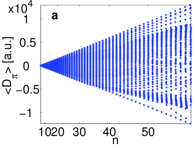
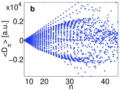
Figure 13: Expectation value of the dipole operator $D_{\pi}$ plotted against the principle quantum number $n$ for different gradients (a: $b=10^{-10}$, b: $b=10^{-8}$).

However, the expectation value of $D_{\pi}$ is in general non-zero. $\left<D_{\pi}\right>$ is shown in figure 13(a,b) for the two gradients $b=10^{-10}$ and $b=10^{-8}$, respectively. For $b=10^{-10}$ the electric dipole moments belonging to the same $n$-multiplet are arranged along vertical lines, which is a result of the approximate degeneracy of the energy levels. The substates for fixed $m$ of a given $n$-multiplet exhibit different dipole momenta spreading between two (upper and lower) bounds that depend linearly depending on $n$. States with a large electric dipole moment emerge from field-free states (with increasing $b$) that possess small values for the angular momentum and vice versa. With increasing gradient and degree of excitation the $n$-mixing starts and disturbs the observed regular pattern. For $b=10^{-8}$ and $n>35$ the distribution of the dipole moments becomes completely irregular. Therefore we encounter the remarkable effect that the external magnetic quadrupole field induces a state dependent permanent electric dipole moment. This is the result of the asymmetric form of the wavefunction in the quadrupole field (see discussion in section VI.3 and figure 4). Exciting the atom from the ground to a corresponding excited state via lasers with the corresponding transition frequency it is therefore possible to prepare an atom with a desired permanent electric dipole moment !

VII Conclusion and Outlook

We have presented a detailed study of the electronic structure of atoms in a magnetic quadrupole field. Opposite to the common adiabatic description of the atomic center of mass motion in inhomogeneous magnetic fields we have focussed on the internal electronic states of the atoms exposed to the inhomogeneous field. We have employed an effective one-particle approach including both the coupling of the electric charge and the magnetic moment (spin) to the field. A spinor-orbital based method to compute the eigenfunctions of the stationary Schrödinger equation has been developed and applied. We have utilized a ’Sturmian’ basis set to study several thousands of excited states for a regime of gradients of more than $10$ orders of magnitude. Due to the inhomogeneity of the quadrupole field the spatial and spin degrees of freedom are coupled in a unique way. As a result the system is invariant under a number of symmetry operations acting on both degrees of freedom. These are the unitary symmetries related to the conservation of the total angular momentum $J_{z}$ and the discrete operation $P_{\phi}OP_{z}$ as well as the anti-unitary generalized time reversal symmetries $TOP_{z}$ and $TP_{\phi}$. These operations constitute a non-Abelian symmetry group which leads to a two-fold degeneracy of each energy level. This is a remarkable feature in particular since it occurs in the presence of the external field. Without a field such (Kramers) degeneracies of a spin-$\frac{1}{2}$-particle are well-known.

We have shown energy spectra up to excitation energies corresponding to principal quantum numbers of $n\approx 60$. The spectrum exhibits distinct characteristics for the weak, intermediate as well as the strong gradient regime. At weak gradients a linear splitting of the energy levels is observed. For given $m$ the sublevels of an $n$-multiplet split symmetrically around the zero field energy. For the homogeneous field a splitting in only two branches is observed due to the two energetically different orientations of the electronic spin. Employing higher gradients adjacent $n$-manifold are still separated but we encounter intra $n$-manifold mixing. Scaling relations for the onset of the intra- as well as the inter $n$-manifold mixing in a quadrupole field have been given. To understand some general features of the effects generated by the quadrupole field we have studied the spectrum of low excitations in very strong (experimentally not accessible) gradients. We have found that the ground state energy virtually stays the same up to gradients of $b=10^{-2}$ whereas the first few excited states already experience severe changes. The latter obviously only holds for hydrogen. However, one way to proceed is to investigate Rydberg states of nonhydrogenic atoms in detail. Here especially scattering with the inner electron shell leads to modifications of the energy spectra which can be understood by quantum defect theory Schmelcher98 ; Wang91 . At least for Rydberg states which possess a large angular momentum we do not expect significant modifications induced by core scattering processes.

In our investigation of the electronic spin properties we found the $S_{z}$-expectation values of the electronic states to form a regular pattern at low gradients. For higher gradients and/or higher excitations we observe a transition to an irregular, much narrower, distribution. In order to analyze the spatial behavior of the electronic spin we introduced the $S_{z}$-polarization. Due to the unique coupling of the spatial and spin degrees of freedom this quantity reveals a rich nodal structure. At low radii we observe a chess-board like pattern of islands with alternating spin polarization changing to a striped pattern at large radii. For Rydberg states the chess board pattern changes to an irregular network of islands exhibiting opposite spin polarizations. Within the striped region an envelope behaviour of the spin orientation on the angle $\theta$ is observed. To investigate this phenomenon we have studied a Hamiltonian describing the coupling of the electronic spin to the magnetic field, neglecting the spatial dynamics. Analytically calculating its eigenstates we could reproduce the above mentioned $\theta$-dependence of the $S_{z}$-polarization of Rydberg-states for large radii.

We have derived selection rules for electromagnetic dipole transitions among eigenstates to the $J_{z}$ as well as $TOP_{z}$ operator. Linearly polarized transitions take place only between states with the same quantum number $m$ or states with different $TOP_{z}$ symmetry. Furthermore we have calculated the amplitudes for $\pi$- and $\sigma^{-}$-transitions emerging from the ground states ($m=\frac{1}{2}$) to levels lying in the intra and inter $n$-manifold mixing regime. We have compared the results with those of a homogeneous magnetic field discovering significant differences in the line structure. Due to additional selection rules arising from the conservation of $z$-parity fewer transitions are observed in a homogeneous magnetic field. Calculating the expectation value of the dipole operator it turned out that the electric dipole moment of the electronic states in the quadrupole field is in general nonzero. For low degrees of excitation and low gradients we observed an almost linear increase of the maximum dipole moment of the $n$-multiplets. This pattern becomes increasingly distorted when moving to higher gradients and/or a higher degree of excitation. The non-vanishing dipole moment is a result of the spatially asymmetric arrangement of the electronic wavefunction with respect to the $x-y$-plane.

In order to achieve the experimental realization of the discussed system the so called atomchip Folman02 seems to be a promising device. Here current carrying nano-structures with dimensions in the $\mu m$-regime can generate high gradient quadrupole fields. At the moment gradients such as $b=10^{-10}$ or even slightly above represent certainly the limit. However, almost all effects discussed here are not due to the diamagnetic interactions but have their origin in the interplay between the Coulomb as well as the spin-spatial Zeeman terms. Therefore weak gradients should not represent a principle obstacle to experimentally observe the derived properties. In particular the magnetic field-induced permanent electric dipole moments would potentially find applications in e.g. quantum information processing Lukin01 ; Jaksch99 ; Calarco00 ; Eckert02 . Exciting the atom from the ground to a corresponding excited state via lasers with the corresponding transition frequency it is possible to prepare an atom with a desired permanent electric dipole moment. In order to build a working two qubit gate one is interested in finding ways to establish a controlled interaction between two qubits to gain a phase shift. Considering a trapped Rydberg state as a qubit the interaction between two of them can be realized via dipole-dipole interaction. This interaction could be switched on and off on demand by changing the atomic state in the quadrupole field.

Taking into account the finite mass of the nucleus it has been shown Avron78 ; Johnson83 ; Schmelcher94 that the center of mass (CM) and electronic motion do not separate i.e. do not decouple in the presence of a homogeneous magnetic field. To enter the corresponding regime where the residual coupling becomes important certain parameter values (excitation energy, CM energy etc.) have to be addressed. A variety of intriguing phenomena due to the mixing of the electronic and CM motion have been observed consequently. Examples are the classical diffusion of the CM due to its coupling to the chaotic internal motion Schmelcher92 , the giant dipole states of moving atoms in magnetic fields Dippel94 as well as the the self-ionization process Schmelcher95a ; Schmelcher95b ; Melezhik00 due to energy flow between the CM and electronic degrees of freedom. In the present investigation we have fixed the position of the CM of the atom at the center of the quadrupole field i.e. we have adopted an infinitely heavy nucleus. On the other hand assuming that an experimentally prepared atom is ultracold will certainly minimize the CM motional effects. Nevertheless, a residual coupling is unavoidable and its impact on the electronic structure is, at this point, simply unknown: A full treatment of the two-body system certainly goes beyond the scope of the present investigation and requires both from the conceptual as well as computational point of view major investigations. However, one should note that the symmetries discussed here equally hold for the moving two-body system i.e. the total angular momentum is conserved and the unitary as well as antiunitary spin-spatial symmetries, now applied to both particles, are also present.

VIII Acknowledgments

We thank Ofir Alon for fruitful discussions regarding the symmetry properties of the atom in the magnetic quadrupole field. I.L. acknowledges a scholarship by the Landesgraduiertenförderungsgesetz of the country Baden-Württemberg.

References

- (1) H. Friedrich and D. Wintgen, Phys. Rep. 183, 37 (1989)
- (2) H. Ruder et al, Atoms in Strong Magnetic Fields, Springer 1992
- (3) H. Friedrich and B. Eckhardt (eds.), Classical, Semiclassical and Quantum Dynamics in Atoms, Lecture Notes in Physics 485, Springer Verlag Heidelberg 1997
- (4) Atoms and Molecules in Strong External Fields, ed. by P. Schmelcher and W. Schweizer, Plenum Press 1998
- (5) Atoms and Molecules in Intense Fields, Eds. L.S. Cederbaum, K.C. Kulander and N.H. March, Springer Series: Structure and Bonding 86, 27 (1997)
- (6) R. Folman et al, Adv. At. Mol. Opt. Phys. 48, 263 (2002)
- (7) I. Lesanovsky, J. Schmiedmayer and P. Schmelcher, Europhys. Lett. 65, 478 (2004)
- (8) T.H. Bergeman et al, J. Opt. Soc. Am. B 6, 2249 (1989)
- (9) W. E. Lamb, Phys. Rev. 85, 259 (1959)
- (10) J. E. Avron, I. W. Herbst and B. Simon, Ann. Phys. (N.Y.) 114, 431 (1978)
- (11) B. R. Johnson, J. O. Hirschfelder and K. H. Yang, Rev. Mod. Physics 55, 109 (1983)
- (12) P. Schmelcher, L. S. Cederbaum an U. Kappes, Conceptual Trends in Quantum Chemistry, p. 1-51 (1994), Eds. E. S. Kryachko and J. L. Calais, Kluwer Academic Publishers
- (13) P. Schmelcher and L. S. Cederbaum, Phys.Lett. A 164, 305 (1992)
- (14) O. Dippel, P. Schmelcher and L. S. Cederbaum, Phys. Rev. A 49, 4415 (1994)
- (15) F. Haake, Quantum Signatures of Chaos, Springer (2001)
- (16) Attila Szabo, Neil S. Ostlund, Modern Quantum Chemistry: Introduction to Advanced Electronic Structure Theory, (Dover, 1996)
- (17) M. Abramowitz and A. Stegun, Handbook of mathematical functions, 5. Dover Edition (Dover Publications, Inc. , New York, 1968)
- (18) D. C. Sorensen, Implicitly restarted Arnoldi/Lanczos methods for large scale eigenvalue calculations in: D. E. Keyes, A. Sameh, V.Venkatakrishnan eds., Parallel numerical algorithms. Dordrecht, Kluwer, 1995
- (19) R. G. Newton, Scattering theory of waves and particles, (Springer, 1982)
- (20) C. W. Clark and K. T. Taylor, J. Phys. B: At. Mol. Phys 13, L737-L743 (1980)
- (21) C. W. Clark and K. T. Taylor, J. Phys. B: At. Mol. Phys 15, 1175-1193 (1982)
- (22) P. Schmelcher and L.S. Cederbaum, Phys. Rev. Lett 74, 662 (1995)
- (23) P. Schmelcher, Phys. Rev. A 52, 130 (1995)
- (24) V. S. Melezhik and P. Schmelcher, Phys. Rev. Lett. 84, 1870 (2000)
- (25) Q. Wang and C. H. Greene, Phys. Rev. A 44, 1874 (1991)
- (26) M.D. Lukin et al, Phys. Rev. Lett. 87, 037901 (2001)
- (27) D. Jaksch et al, Phys. Rev. Lett. 82, 1975 (1999)
- (28) T. Calarco et al, Phys. Rev. A 61, 022304 (2000)
- (29) K. Eckert et al, Phys. Rev. A 66, 042317 (2002)